One-Class-Based Uncertain Data Stream Learning Bo Liu∗
Yanshan Xiao†
Longbing Cao‡
Abstract This paper presents a novel approach to one-class-based uncertain data stream learning. Our proposed approach works in three steps. Firstly, we put forward a local kerneldensity-based method to generate a bound score for each instance, which refines the location of the corresponding instance. Secondly, we construct an uncertain one-class classifier by incorporating the generated bound score into a one-class SVM-based learning phase. Thirdly, we devise an ensemble classifier, integrated from uncertain one-class classifiers built on the current and historical chunks, to cope with the concept drift involved in the uncertain data stream environment. Our proposed method explicitly handles the uncertainty of the input data and enhances the ability of oneclass learning in reducing the sensitivity to noise. Extensive experiments on uncertain data streams demonstrate that our proposed approach can achieve better performance and is highly robust to noise in comparison with state-of-the-art one-class learning method. 1 Introduction One-class learning on uncertain data streams is a new and challenging research issue. It involves the consolidation of one-class learning [1], data stream mining [2], and uncertain data learning [3]. The problem-solving nature of many real-life applications, such as sensor network, and intrusion detection, can be categorized as one-class-based uncertain data stream learning. In one-class learning, only one class of samples is labeled in the training phase [1]. The labeled class is typically called the target class, while all other samples not in this class are defined as the non-target class. The purpose of one-class learning is to build a distinctive classifier to decide whether a test instance belongs to the target class or the non-target class. Such one-class classification problems, often referred to as outlier detection or text classification, have wide real-world applications, typically in intrusion ∗ QCIS Centre, Faculty of Engineering and IT, University of Technology, Sydney. Email:
[email protected] † QCIS Centre, Faculty of Engineering and IT, University of Technology, Sydney. Email:
[email protected] ‡ QCIS Centre, Faculty of Engineering and IT, University of Technology, Sydney. Email:
[email protected] § Department of Computer Science, University of Illinois at Chicago, 851 S. Morgan Street, Chicago, IL 60607-0753. Email:
[email protected]
992
Philip S. Yu§
detection, fraud detection, churn management, and Web page classification [4, 5]. The one-class SVM (OC-SVM) [6] is one of the bestknown support vector learning methods [7] for one-class classification problems. In OC-SVM, the original data are mapped from the input space into a higher dimensional feature space, in which the inner products of the two vectors can be directly calculated using a kernel function [8]. In the feature space, OC-SVM determines a hyperplane to separate the target class and the origin of the feature space with the maximum margin. The learned hyperplane is thereafter used as a predictive model to classify data into the target or nontarget class. In general, OC-SVM outperforms Gaussiandensity based linear classifier and Parzen classifier for oneclass classification problems [1]. Despite much progress in this area, most of the existing work on one-class classification has not explicitly dealt with the uncertainty of the input data. They are based on an underlying assumption that the training data set does not contain any uncertainty information. However, data in many real-world applications is uncertain in nature. This is because data collection methodologies are only able to capture a certain level of information, making the extracted data incomplete or inaccurate [3]. For example, in environmental monitoring applications, sensor networks typically generate a large amount of uncertain data because of instrument errors, limited accuracy or noise-prone wireless transmission [3]. In other cases, data points extracted in a business may only correspond to business objects that are vaguely specified, which makes the extracted data representation uncertain. This kind of uncertain information, typically ignored in most of the existing one-class learning methods, is critically important for capturing the full picture of the underlying data. It should be considered in the learning phase in order to build a classifier that fully reflects the nature of data. Recently, advanced data stream technologies have been used to process large amounts of high frequency data [2, 9, 10]. Due to its potential in industry applications, data stream mining has been studied intensively. One characteristic of data streams is the evolution of data concepts (also called concept drift [2]). Meanwhile, a large volume of one-class data, such as sensor network and intrusion detection data, is increasingly collected in a data stream environment which raises the challenging research issue of one-class learning on data streams. An even more challenging issue is to
Copyright © SIAM. Unauthorized reproduction of this article is prohibited.
learn one-class classifiers on uncertain data streams. This is because the presence of uncertain data and concept drift in data streams always makes one-class learning far more difficult than traditional data stream learning methods and uncertain data learning. In this paper, we address the problem of one-class learning on uncertain data streams. We propose a novel approach, which is called uncertain one-class learning (UOCL) framework, which copes with the data uncertainty and the concept drift in one-class-based uncertain data streams. UOCL first assigns a bound score to each instance to estimate the range of uncertainty and then incorporates the uncertainty information into the one-class learning phase. The main contributions of our work are summarized as follows. 1. We propose a local kernel-density-based mechanism to generate a bound score for each instance by investigating its local nearest neighbors in the feature space. By using the generated bound score, we estimate the range of uncertainty such that we can refine the location of the uncertain instance in the learning phase. 2. To cope with data uncertainty, the generated bound score is thereafter incorporated into the OC-SVM learning phase to build an uncertain one-class classifier (UOCC). In this phase, we propose the usage of an interactive framework to mitigate the effect of noise on the one-class classifier. To the best of our knowledge, this is the first time to explicitly handle data uncertainty in one-class uncertain data streams.
Table 1: Notion and meaning Notions OC-SVM S |S| xi x, n ∥ x1 − x2 ∥ x1 · x1 ϕ(.) F ϕ(x) K(., .) w v ξi ρ Data stream Dt |Dt | P Dt U Dt ft gt fE △xi δi xsi Sk (xi ) Dav xi M ε αi Experiment σi0 vj xi + vj η
Meaning training set training set size the ith training example input space, n = dim(x) distance between x1 and x2 inner product of two vectors non-linear mapping function feature space image of x in feature space kernel function normal vector of hyperplane control parameter slack-variable for ith training sample hyperplane: ρ = w · x data stream chunk between t − 1 and t sample size of the chunk t subset of Dt , containing labeled target examples subset of Dt , consisting of unlabeled examples the classifier built on the Dt chunk weight of classifier ft ensemble classifier noise vector associated with xi bound score of ∥ △xi ∥ such that ∥ △xi ∥≤ δi original uncorrupted input: xsi = xi + △xi k-nearest neighbors set of instance xi average distance between xi and its K neighbors distance matrix threshold Lagrange multipliers standard deviations of source data along dimension i. random vector associated with xj corrupted data noise lelve
3. We introduce the usage of ensemble classifiers which are derived from the current and historical chunks to handle concept drift in uncertain data streams. By using the ensemble classifier, we can capture the evaluation of uncertain data streams, we first review the previous methods concept drift in the data stream environment. for learning uncertain data in Section 2.1, and then briefly 4. We conduct extensive experiments to evaluate the per- introduce one-class learning in Section 2.2.
formance of our proposed UOCL framework. The statistical results show that UOCL outperforms state-of- 2.1 Mining Uncertain Data Recently, many advanced the-art one-class learning method in terms of perfor- techniques have been developed to collect and store large quantities of data. Some records in the data may be intermance and sensitivity to noise added into data. rupted by noise, leading to missing or partially complete data For clarity, Table 1 lists the notations used in this paper. [3]. In such cases, the data objects may be only vaguely The rest of the paper is organized as follows. Section 2 specified and are therefore considered uncertain in their repdiscusses previous work related to this paper. Section 3 intro- resentation [3]. The presence of uncertain data has created duces the preliminaries of our study. Section 4 presents our a great need for uncertain data algorithms [3, 11, 12, 13]. proposed approach to one-class-based uncertain data stream From the application perspective [3], we briefly review the learning. Section 5 reports substantial experimental results previous work on clustering, classification, frequent pattern on mining uncertain data streams. Section 6 concludes the mining and outlier detection on uncertain data. paper and discusses possible directions for future work. SecFor the clustering methods with uncertain data, most of tion 7 is the Appendix. them typically extend original clustering methods to cope with data uncertainty. The representative methods are intro2 Related work duced as follows. FDBSCAN [14], developed on DBSCAN In this Section, we briefly review previous work related [15], probabilistically specifies the uncertain distances beto our study. Since our focus is one-class learning in tween objects to find density-based clusters from uncertain
993
Copyright © SIAM. Unauthorized reproduction of this article is prohibited.
data. FOPTICS [16] introduces a fuzzy distance function to measure the similarity between uncertain data on top of the hierarchical density-based clustering algorithm. UK-means [17], built on the K-means method, assigns an object to the cluster whose representative has the smallest expected distance from the object. Aggarwal [18] proposes the use of density-based approaches to handle error-prone and missing data. The above methods on uncertain data are developed for static uncertain data. Recently, the problem of clustering uncertain data streams has been discussed in [19], which incorporates error statistics and the micro-clustering concept [20] to cope with dynamic uncertain data. For the classification methods on uncertain data, the standard binary SVM is extended to handle uncertain data [21, 22, 23]. These methods provide a geometric algorithm which optimizes the probabilistic separation between the two classes on both sides of the boundary. Moreover, frequent pattern mining on uncertain data is investigated in [24], in which the probability of an item belonging to a particular transaction is typically modeled. In addition, outlier detection with uncertain data has been studied in [25], which draws multiple samples from the data and computes the fraction of the samples. Despite much progress on uncertain data mining, most of the previous work has not explicitly dealt with one-class learning on uncertain data. This paper proposes an uncertain one-class learning (UOCL) framework to cope with data uncertainty and concept drift in data streams. In this framework, uncertain one-class classifier (UOCC) extends standard the OC-SVM for uncertain data. Although UOCC is a support vector method, it is different from uncertain binary SVM [21, 22, 23]. Firstly, we propose a local kerneldensity-based mechanism to generate a bound score for each instance. Secondly, we simplify our optimization problem (4.9) into a standard QP (quadratic programming) optimization problem (4.11) by considering the characteristic of oneclass learning. Thirdly, the UOCC method is embedded into data streams to cope with concept drift. 2.2 One-Class Learning The previous work on one-class learning can be classified into two broad categories. For the methods in the first category [26, 27, 28], they are developed mainly for document-related one-class classification problems. Their main task is to extract negative samples from unlabeled examples (if unlabeled examples are offered) and to construct a binary classifier using target samples and extracted negative samples. The advantage of these methods is that they can well resolve document-related one-class classification problems. In the second category, OC-SVM and support vector data description (SVDD) are representative methods [6, 1]. Both methods aim to constructe a one-class classifier using only the target class. The advantage of these methods is
994
that they can cope with any one-class classification problem. In this paper, we study one-class learning in this category. Because OC-SVM and SVDD have been proved to have the same decision classifier [1], we briefly introduce OC-SVM [6] as follows. Suppose the training target class is S = {x1 , x2 , . . . , x|S| }, where xi ∈ Rn . In the input space, OC-SVM aims to determine a hyperplane to separate the target class and the origin of the input space with the maximum margin: |S|
min s.t. (2.1)
1 ∑ 1 ∥ w ∥2 −ρ + ξi 2 v · |S| i=1 w · xi ≥ ρ − ξi ξi ≥ 0, i = 1, 2, . . . , |S|,
where parameter v is used to tradeoff the sphere volume ∑|S| and the errors i=1 ξi . After resolving problem (2.1) by introducing a Lagrangian function [7], w and ρ = w · x can be obtained. For a test sample xt , if (2.2)
w · xt > ρ,
it is classified into the target class; otherwise, it belongs to the non-target class. In addition, the kernel method is adopted to offer a more flexible ability of OC-SVM. In this case, the input data are mapped into a feature space, in which the inner product of two vectors ϕ(x) and ϕ(xi ) can be calculated by a kernel function K(x, xi ) = ϕ(x) · ϕ(xi ). Among a variety of kernel functions, RBF kernel is a typical: (2.3)
2
K(x, xi ) = exp(−∥ x − xi ∥2 /2σ 2 ).
The original OC-SVM can not cope with the one-class classification problem with uncertain data, which potentially limits its performance. Another disadvantage of OC-SVM is that it is developed on static data and can not deal directly with the concept drift in data streams. In this paper, we refine the formulation of the original OC-SVM to handle uncertain data, and propose the usage of an ensemble classifier to cope with concept drift in data streams. 3 PRELIMINARY 3.1 Problem Definition Suppose we have a series of data streams D1 , D2 , . . . , Dm , in which each Dt (t = 1, 2, . . . , m), called “chunk”, contains the data that arrived between time tt−1 and tt . Here Dc is called the current chunk and the yet-to-come data chunk (denoted as Dc+1 ) is dedicated as the target chunk. In the current chunk Dc , the labeled examples are put into set P Dc . Other examples, including non-labeled target
Copyright © SIAM. Unauthorized reproduction of this article is prohibited.
We let xi + △xi (∥ △xi ∥≤ δi ) denote the reachability area of instance xi as illustrated in Figure 1. We then have
Reachabitily Area
∥ xsi ∥ = ∥ xi + △xi ∥≤∥ xi ∥ + ∥ △xi ∥
xi
(3.6) | xi| Origoi n
Figure 1: Illustration of reachability area of instance xi . class examples and non-target class examples, are put into set U Dc . The objective of one-class data streams is to build a classifier around the labeled target class examples P Dc , and predict the data label in the yet-to-come chunk. For one-class-based uncertain data streams, we have the following assumption: only instances in the current chunk Dc are accessible, and once the algorithm moves from chunk Dc to chunk Dc+1 , all instances in chunk Dt , 1 ≤ t ≤ c, are inaccessible; we can only use the models trained from the historical chunks. This is because aggregating historical data always requires extra storage, and most data stream mining algorithms are required to make predictions based on onescanning of the data streams without referring to historical data. 3.2 Uncertainty Model For the labeled class in the current chunk, that is P Dc , we assume each input data xi is subject to an additive noise vector △xi . In this case, the original uncorrupted input xsi is denoted (3.4)
xsi = xi + △xi .
In theory, we can assume △xi follows a certain distribution. However, in practice, we may not have any prior knowledge on the noise distribution. Alternatively, the method of bounded and ellipsoidal uncertainties has been investigated in [22, 29]. In this situation, we consider a simple bound score for each instance such that: (3.5)
∥ △xi ∥≤ δi .
Actually, this setting has a similar effect of assuming △xi has a certain distribution. For example, if we assume △xi follows a Gaussian noise model, that is
≤ ∥ xi ∥ +δi
In this way, xsi falls in the reachability area of xi . By using the bound score for each input sample, we can convert the uncertain one-class learning into standard oneclass learning with constraints. We will introduce bound score determination for each instance in Section 4.1 and how to incorporate uncertainty information into the learning phase in Section 4.2. 4 Proposed Approach In this Section, we provide a detailed description about our proposed approach. Subject to sampling errors or device imperfections, the instance in the one-class-based data streams is always considered uncertain in its representation. Another characteristic of one-class-based data streams is concept drift, which indicates that a user’s interest will change as time goes by. These two challenges make one-class-based uncertain data stream learning much more difficult than traditional ones. To deal with the data uncertainty and concept drift in one-class-based uncertain data stream learning, we propose the uncertain one-class learning (UOCL) framework, as illustrated in Figure 2. The UOCL framework works in three steps: • In the first step, we generate a bound score for each instance in P Dc based on its local data behavior. • In the second step, we incorporate this generated bound score into the learning phase to interactively build an uncertain one-class classifier (UOCC). • In the third step, we integrate the uncertain oneclass classifiers derived from the current and historical chunks to predict the data in the target chunk. In the following, we exhibit the three steps in detail. For simplicity, we detail the bound score determination and uncertain one-class classifier construction for the current chunk Dc . We can generalize the two operations on other chunks.
4.1 Step One: Bound Score Determination In practice, we are unlikely to know the distribution of △xi , and it will 2 ∥xi −xs i∥ be difficult to exactly determine the bound score for each p(|xi − xsi |) ∼ exp 2σ2 , instance. One simple solution is to let users set the parameter The bound δi has a similar influence of the standard deviation δi themselves. For example, the work in [22] sets a uniform δ σ in the Gaussian noise model. In addition, the squared for each instance in uncertain binary classification. However, ∥x −xs ∥2 penalty term i2σ2i is replaced by a constraint ∥ △xi ∥≤ this setting will greatly challenge users, since a big value of δi . δi will be meaningless. For example, if we set δi = ∞, any
995
Copyright © SIAM. Unauthorized reproduction of this article is prohibited.
fE Step3: Classifiers ensemple
xi xi
Step2: UOCC construction Step1: Boundscore determination
Predict
Ensemble Classifier
f c-l-1
Bound Score
D c-l-1
f c-l
Bound Score
D c-l
f c-1
Bound Score
fc
Bound Score
D c-1
DS ct
D c+1 (A)
Figure 2: Illustration of one-class-based uncertain data stream learning framework. The ensemble classifier fE is built on the classifiers (fc−l−1 , fc−l , . . . , fc ) derived from l chunks. noise △xi will satisfy ∥ △xi ∥≤ ∞, but this setting will not make sense for the solution. To cope with this challenge, we propose a local kerneldensity method to generate a bound score for each instance by examining its local neighbors in a kernel feature space. More specifically, we first identify the k nearest neighbors of instance xi in the feature space. The distance between xi and xj in the feature space is computed as
(B)
Figure 3: (A): Illustration of four nearest neighbors’ range (inner rectangle) and twelve nearest neighbors’ range (outer rectangle) of instance xi . (B): Reachability area of instance xi in terms of four nearest neighbors (inner circle) and twelve nearest neighbors (outer circle).
computed by four nearest neighbors (inner circle in the right figure). In all, the local kernel-density-based method is given in Algorithm 1.
4.2 Step Two: Uncertain One-Class Classifier Construction After generating a bound score for each instance in P Dc , the next step is to build an uncertain one-class clas(4.7) sifier to cope with uncertain data. √ Below, we give a new formulation of OC-SVM by ∥ ϕ(xi ) − ϕ(xj ) ∥= K(xi , xi ) + K(xj , xj ) − 2K(xi , xj ). incorporating uncertainty into the learning phase. We then calculate the average distance of xi to its k nearest 4.2.1 Primal Formulation Based on the bound score for neighbors as follows. each instance, the formulation of the standard OC-SVM |Sk(xi ) | (Optimization problem (2.1)) is extended as follows. ∑ 1 (4.8)Dav (xi ) = ∥ ϕ(xj ) − ϕ(xi ) ∥, |Sk(xi ) | j=1 |P Dc | ∑ 1 1 2 min ∥ w ∥ −ρ + ξi where Sk(xi ) is the k nearest neighbors set of xi . 2 v · |P Dc | i=1 In general, the smaller the Dav (xi ), the greater the s.t. w · (xi + △xi ) ≥ ρ − ξi density on instance xi in feature space. ξi ≥ 0, ∥ △xi ∥≤ δi We then let δi = Dav (xi ). The motivation behind this i = 1, 2, . . . , |P Dc |. setting is that: if a normal instance is corrupted by noise (4.9) such that it resides far from other normal examples, we use this setting to ensure the reachability area of xi can reach the In problem (4.9), the method of modeling noise lets UOCC regions other normal examples cover. As illustrated in Figure less sensitive to the sample corrupted by noise since we can 3, assume xi is corrupted by noise, the inner rectangle in the determine a choice of △xi to render xi + △xi far from the left figure covers the four-nearest neighbors of xi , and the decision boundary learned from the OC-SVM. As illustrated corresponding reachability area of xi (inner circle in the right in Figure 4, x1 and x2 are corrupted samples: assume the figure, calculated using four nearest neighbors) can reach the dash line is the classifier learned from the standard OCregions other normal examples cover. SVM, after incorporating x1 + △x1 and x2 + △x2 into the Intuitively, a large k will result in a large reachability learning phase, we obtain the refined boundary denoted by a area of xi . As illustrated in Figure 3, the reachability area solid line. In this case, the hyperplane learned from problem of xi calculated using twelve nearest neighbors (outer circle (4.9) is less sensitive to uncertain data compared with that in the right figure) can cover a much greater area than that derived from the original problem (2.1).
996
Copyright © SIAM. Unauthorized reproduction of this article is prohibited.
Algorithm 1 Local kernel-density-based method. Input: P Dc ; // positive set in current chunk Dc ........... k; // number of neighbors ........... K(., .). // kernel function Output: δi .// bound score
refined boundary
x1 Initialize distance matrix M|P Dc |∗|P Dc | = 0; 2: for i = 1 to |P Dc | do for j = i + 1 to |P Dc | do 3: x2 4: Calculate Mij =∥ ϕ(xi ) − ϕ(xj ) ∥ via Equation (4.7); Origoi n 5: Let Mji = Mij ; 6: end for origni al boundary Identify the k nearest neighbors of instance xi and put 7: them into set Sk(xi ) ; 8: end for Figure 4: Decision boundaries of the standard OC-SVM and 9: for i = 1 to |P Dc | do UOCC methods. 10: Calculate Dav (xi ) via Equation (4.8); 11: Let δi = Dav (xi ); We then have Theorem 2 to solve the optimization 12: end for problem (4.11) as follows. 13: Return δi . Theorem 2: By using Lagrangian function [7], the solution of the optimization problem (4.11) is to resolve the following 4.2.2 Solution to UOCC To solve the problem (4.9), we dual problem use an iterative approach to calculate ρ and △xi . More |P Dc | |P Dc | 1 ∑ ∑ specifically, we first fix each △xi and solve problem (4.9) αi · αj (xi + △xi ) · (xj + △xj ) F (α) = min to obtain ρ, and then fix ρ to calculate △xi iteratively. We 2 i=1 j=1 1 detail the approach as follows . 1 First of all, we have the following Lemma. s.t. 0 ≤ αi ≤ v · |P Dc | Lemma 1: For a given hyperplane, denoted as ρ = w · x, the |P D | solution of problem (4.9) over △xi is ∑c (4.12) αi = 1 i = 1, 2, . . . , |P Dc |, w i=1 (4.10) . △xi = δi ∥w∥ and This Lemma indicates that, for a given w, the minimization |P Dc | of problem (4.9) over △xi is quite straightforward. ∑ w = αi · (xi + △xi ) (4.13) We have the Theorem 1 to update w and ρ when △xi is i=1 temporally fixed. Theorem 1: If optimal △xi = δi w/ ∥ w ∥ (i = (4.14) ρ = w · x, 1, 2, . . . , |P Dc |) is fixed, the solution of problem (4.9) over where αi is the Lagrange multipliers. This theorem indicates w and ρ is equivalent to that the solution of problem (4.12) is a standard dual problem |P Dc | by treating xi + △xi as a new instance, i.e, x′ = xi + △xi . ∑ 1 1 2 ∥ w ∥ −ρ + min ξi By referring to the alternating optimization method in 2 v · |P Dc | i=1 [29], we propose the usage of the iterative approach to resolve problem (4.9) in Algorithm 2. s.t. w · (xi + △xi ) ≥ ρ − ξi In Algorithm 2, ε is a threshold. Since the value ξi ≥ 0, of Fval (t) is nonnegative, with the decreasing of Fval (t), (4.11) i = 1, 2, . . . , |P Dc |. |Fval (t) − Fval (t − 1)|/|Fval (t − 1)| will be smaller than This Theorem indicates that we can release the constraint a threshold. ∥ △xi ∥≤ δi in problem (4.9) to simplify the optimization. 4.2.3 Extension to Kernel-Based UOCC In OC-SVM, 1 For the deviation of the Lemma and Theorem 1, please see Section 7 in kernel method always offers a more accurate classifier for detail. one-class classification problem. In such case, each input 1:
997
Copyright © SIAM. Unauthorized reproduction of this article is prohibited.
Algorithm 2 Uncertain one-class classifier construction Input: P Dc ; // positive set in current chunk Dc ........... v. // parameter of one-class SVM. ........... δi // bound value for each sample. Output: ρ. 1: Initialize each △xi = 0; 2: t=0; 3: Initialize Fva (t) = ∞; 4: repeat 5: t = t + 1; 6: Fix △xi for i = 1, 2, . . . , |P Dc | and solve problem (4.12); 7: Let Fva (t) = F (α); Obtain αi , i = 1, 2, . . . , |P Dc |; 8: ∑P D 9: Obtain w = i=1c αi · (xi + △xi ) and hyperplane ρ = w · (x); 10: Fix w and resolve optimization problem (4.9) to update each △xi according to Equation (4.10); 11: until |Fva (t) − Fva (t − 1)| < ε|Fva (t − 1)| 12: Return ρ = w · xi .
Algorithm 3 Main procedure of UOCL Framework Input: Dc ; // Current chunk ........... K(., .) // kernel function ........... fi (i = c − l + 1, c − l + 2, . . . , c) // historical classifiers Output: fE //ensemble classifier 1: 2: 3: 4: 5: 6: 7: 8:
Collect P Dc from Dc ; Call Algorithm 1 to calculate δi ; Call Algorithm 2 using kernel method to obtain fc ; for i = 1, i ≤ l, i + + do Calculate the classifier weight gi for classifier fi end for Combine fi (i = c − l + 1, c − l + 2, . . . , c) to form ensemble classifier fE ; Return fE .
4.2.4 Computation Complexity Analysis The computation complexity of problem (4.12) is O(|P Dc |)2 . The update of xi in (4.10) just needs linear time, that is O(|P Dc |). instance x is mapped into a feature space via mapping Suppose the iterative approach stops after m times iterations. function ϕ(.), and the image of x in feature space is ϕ(x). To The computation complexity of resolving problems (4.9) and obtain kernel-based UOCC, we just need to replace xi + △xi (4.15) is m · O(|P Dc |)2 + m · O(|P Dc |). with ϕ(xi + △xi ) in optimization problem (4.9) such that 4.3 Step Three: Ensemble Classifiers After building un|Dc | ∑ 1 1 certain one-class classifiers on the current and historical 2 ξi min ∥ w ∥ −ρ + 2 v · |Dc | i=1 chunks, we obtain fc−k+1 , fc−k , . . . , fc . To cope with concept drift in data streams, we combine these k classifiers to s.t. w · ϕ(xi + △xi ) ≥ ρ − ξi form an ensemble classifier fE to predict instances in the ξi ≥ 0, ∥ △xi ∥≤ δi target chunk. By referring to the method in [2], we assign (4.15) i = 1, 2, . . . , |Dc |. a weight value gi to each individual classifier such that the ensemble classifier fE can be quickly adjusted to the users’ The same as solution of problem (4.9), the solution of current interests. problem (4.15) consists of two steps. In the first step, fix In all, the main framework of the uncertain one-class △xi to obtain w. In the second step, fix learned w and to learning framework is shown in Algorithm 3. optimize △xi . We introduce the two steps as follows. In step one, we fix △xi as a value such that ∥ △xi ∥≤ δi , 5 Performance evaluation and resolve problem (4.12) by replacing (xi + △xi ) · (xj + 5.1 Baseline and Metrics In this Section, we will inves△xj ) with K(xi + △xi , xj + △xj ). We then have tigate the performance of our proposed UOCL approach on P Dc ∑ uncertain data streams. For comparison, the original OC(4.16) w= αi · ϕ(xi + △xi ). SVM is used as a baseline. Since OC-SVM was developed i=1 for static data, we embed it in a data stream environment and ∑P Dc In step two, we fix w = i=1 αi · ϕ(xi + △xi ) and resolve use an ensemble classifier to predict yet-to-come data. This baseline is used to show the improvement of our proposed problem (4.15) over △xi , we have method over the OC-SVM learning method. w The performance of classification systems is typically (4.17) . △xi = δi ∥w∥ evaluated in terms of F-measure [30]. The F measure trades Based on the above two steps, we adopt the same iterative off precision p and recall r: F = 2pr/(r + p). From this approach used in Algorithm 2 to resolve problem (4.15). definition, we know only when both precision and recall After that, we obtain the learned uncertain one-class are large will the F-measure exhibit large value. For the classifier fc = w · x for prediction. theoretical basis of F-measure, please refer to [30] for detail.
998
Copyright © SIAM. Unauthorized reproduction of this article is prohibited.
All the experiments are on a laptop with a 2.8 GHz processor and 3GB DRAM. For both UOCL and OC-SVM, we use Lib-SVM 2 to resolve the standard QP problem. RBF kernel function (2.3) is employed with default parameters.
uncertain pattern
xv
vector
v
z Pattern
5.2 Data set Description In the experiments, we use one synthetic data set and two real-world data sets which have been used by other researchers to generate data streams [19, 31]. The basic information of the used data sets is introduced as follows.
2. KDD-99 3 : This data set was collected from the KDD CUP challenge in 1999, and the task is to build predictive models capable of distinguishing between possible intrusions and normal connections. The original data (10% sampling) contain 41 features, 494,020 training and 311,029 test samples, and over 24 intrusion types. In these types, there exist three large size classes, that are Normal, Neptune, and Smurf classes. The three classes dominate the whole data set. We combine training and testing sets together and use the three large size classes to generate a one-class data stream. 3. Forest CoverType4 : This data set contains 581012 observations and each observation consists of 54 attributes, including 10 quantitative variables, 4 binary wilderness areas and 40 binary soil type variables. Seven classes exist: “Spruce-Fir”, “Lodgepole Pine”, “Ponderosa Pine”, “Cottonwood/Willow”, “Aspen”, “Douglas-fir”, “Krummholz”. We use the seven classes to generate one-class data stream. 5.3 Experiment Setting 5.3.1 Data stream Generation We generate data streams using the above three data sets as follows. For each data set, we first randomly choose one class, and regard it as target class and treat the other categories as 2 Available
at http://www.csie.ntu.edu.tw/ cjlin/libsvm/ at http://kdd.ics.uci.edu/databases/kddcup99/kddcup99.html 4 Available at http://archive.ics.uci.edu/ml/datasets/Covertype 3 Available
999
x
y
1. Synthetic Data: This data set consists of three classes generated using three Gaussian distributions with 10 attributes. We control the mean and standard deviation of each Gaussian distribution such that they won’t overlap too much. Specifically, we set the mean of the three Gaussian distributions as 0, 0.5 and 1, the standard deviation of each Gaussian distribution is drawn from the uniform distribution in the range [0.2, 0.8]. After that, we generate 15000, 25000 and 20000 samples for three classes.
x
Figure 5: Illustration of the method used to add the noise to a data example: x is an original data example, v is a noise vector, xv is the new data example with added noise. Here we have xv = x + v. the non-target class. Take the CoverType data set for example: if we choose the “Spruce-Fir” category as the target class, then the non-target class consists of the “Lodgepole Pine”, “Ponderosa Pine”, “Cottonwood Willow”, “Aspen”, “Douglas-fir” and “Krummholz”. In a sequential time period of the stream environment, we randomly choose a number of examples from the target class and choose examples from the non-target class such that the target class dominates the chosen data. One characteristic of data streams is concept drift. To simulate concept drift in the data stream environment, we employ the following three scenarios: (1) constant concept (CC), (2) regular concept shifting (RCS), and (3) probability concept shifting (PCS). • In the constant model, users will not change their interests across the whole data stream. In this case, we fix the target class so that it is unchanged all the time. For each data set, we use the biggest class as the normal class and treat the other classes as the non-target class. • In the regular shifting model, we regularly shift interest by changing the target class from one class to another, after a fixed number of chunks, and we set this chunk number as 5 in the experiments. At the same time, the non-target class is accordingly changed. For example, if the target class changes from “Spruce-Fir” class to “Lodgepole Pine” in the Forest CoverType data set, the changed non-target class will contain “SpruceFir”, “Ponderosa Pine”, “Cottonwood/Willow”, “Aspen”, “Douglas-fir”, “Krummholz”. • In the probability shifting model, we change the target class with a probability (p). If the generated p is larger
Copyright © SIAM. Unauthorized reproduction of this article is prohibited.
than a threshold (0.5), we change the target class from one class into another class.
100 UOCL
95
Average F−measure value
Average F−measure value
OC−SVM For the majority of experiments in the paper, we use a regular 90 shifting model and a probability shifting model, because they 85 are closer to real-world models. Using the above operation, we generate three data 80 streams for each data set, called CC-based, RCS-based, and 75 PCS-based data streams. For fair comparison, both UOCL and OC-SVM use the same number of classifiers to form the 70 ensembles. We omit the details of the algorithm performance 65 with respect to the chunk size (|Dc |), and the number of en60 semble classifiers (l), because the impact of these factors has been addressed more or less in the stream data mining lit55 erature [2, 9, 10]. Instead, we use chunk size N=1000, en50 CC model RCS model PCS model semble size l=10 for all streams. The purpose of fixing these Three types of models parameters is to fully investigate and compare algorithm perFigure 6: Average F-measure value comparison (Synthetic formance on uncertain data streams. For each chunk Dc , we randomly label a majority data, η = 0.5). of target class examples, i.e., approximately 90% target 90 examples, and consider the remaining target class examples UOCL and non-target class examples as unlabeled examples. The 85 OC−SVM number of k in the bound score determination step is set as 80 |P Dc |/10, and ε is set as 0.15. 75
(5.18)
x
x
Average F−measure value
5.3.2 Noise Generation We note that the artificial and UCI data sets are deterministic, so we need to model and add 70 uncertainty to these data sets. In the following, we introduce 65 noise addition to P Dc ; the same operation can be used on other chunks. 60 Following the method in the previous work [19],we generate the noise using a Gaussian distribution with zero 55 mean and a standard deviation whose parameter was chosen as follows. For each chunk of data streams, we first compute 50 CC model RCS model PCS model the standard deviation σi0 of the entire data in P Dc along the Three types of models ith dimension, and then obtain the standard deviation of the Figure 7: Average F-measure value comparison (KDD-99 Gaussian noise σi randomly from the range [0, 2 · η · σi0 ]. For data, η = 0.5). a generated noise vector, Figure 5 illustrates the basic idea of 75 the method to add the noise vector to a data sample. Specifically, the standard deviation σi0 of the entire data UOCL 70 OC−SVM along the ith dimension is first obtained. In order to model the difference in noise on different dimensions, we define the 65 standard deviation σi along the ith dimension, whose value 60 is randomly drawn from the range [0, 2 · η · σi0 ]. Then, for the ith dimension, we add noise from a random distribution with 55 standard deviation σi . In this way, a data example xj in the 50 target class is added with the noise, which can be presented as a vector 45 x
j σ xj = [σ1j , σ2j , · · · , σn−1 , σnxj ].
Here, n denotes the number of dimensions for a data example x xj , and σi j , i = 1, · · · n represents the noise added into the ith dimension of the data example.
1000
40 35 30
CC model
RCS model
PCS model
Three types of models Figure 8: Average F-measure value comparison (Forest CoverType data, η = 0.5).
Copyright © SIAM. Unauthorized reproduction of this article is prohibited.
11000
Number of data samples processed/sec
10000 OC−SVM UOCL
9000 8000 7000 6000 5000 4000 3000 2000 1000 0
1
1.5
2
2.5 3 3.5 4 Progression of data stream
4.5
5
x 105
Figure 9: Efficiency comparison (Synthetic data, η = 0.5).
Number of data samples processed/sec
7000
OC−SVM UOCL
6000
5000
4000
3000
2000
1000
0
1
1.5
2
2.5 3 3.5 4 Progression of data stream
4.5
5
x105
Figure 10: Efficiency comparison (KDD-99 data, η = 0.5).
Number of data samples processed/sec
7000
OC−SVM UOCL
6000
5000
5.4 Performance Comparison We first investigate the performance of UOCL and OC-SVM in terms of CC-based, RCS-based, and PCS-based uncertain data streams, in which the noise level η is set to 0.5. The average F-measure value of forty chunks in data streams is reported from Figures 6 to 8, in which x− axis illustrates the type of the data streams, and y− axis denotes the average F-measure value for each method. It is clear that in this case, UOCL provides superior performance compared with the standard OC-SVM in terms of CC-based, RCS-based, and PCS-based uncertain data streams. This occurs because UOCL, developed on the OCSVM, can reduce the effect of the noise on the decision boundary such that we can build a more accurate classifier. Another observation from these Figures is that the Fmeasure value obtained from CC-based data streams is typically higher than that of RCS-based and PCS-based data streams. This is because CC-based data streams will not involve concept drift so that each chunk shares identical data distribution. 5.5 Efficiency Comparison To test the efficiency of our UOCL method, we refer to the method in [19] and perform UOCL and OC-SVM on PCS-based uncertain data streams in which noise level η is set 0.5. Figures 9 to 11 illustrate the efficiency of both methods on the three data sets. On the x− axis, we illustrate the progression of the data stream in terms of the number of samples, whereas on the y− axis, we illustrate the number of samples processed per second at particular points of the data stream progression. This number is computed by using the average number of samples processed per second in the last 2 seconds. From these Figures, we find that the original OC-SVM always obtains higher processing speed because it does not mitigate the effect of uncertain data on the classifier construction. Consequently, OC-SVM offers higher processing speed yet inferior performance to UOCL. We further discover that, although UOCL uses an interactive framework to address data uncertainty, the UOCL method is able to process thousands of samples per second in each case. Thus, the UOCL method is not only effective, but is also an efficient one-class method for uncertain data streams.
4000
5.6 Performance Sensitivity on Different Noise Levels So far we have investigated the performance and efficiency of our proposed method. However, it is still interesting to see how the performance of the two methods would be affected under different noise levels. Taking the RCS-based and PCS-based uncertain data streams for example, we increase the noise level from 0.5 to 2. In Figure 12, we illustrate the variation in effectiveness with increasing error. On the x−axis, we illustrate the noise level. On the y−axis, we illustrate the average F-measure
3000
2000
1000
0
1
1.5
2
2.5 3 3.5 4 Progression of data stream
4.5
5
x105
Figure 11: Efficiency comparison (Forest CoverType data, η = 0.5).
1001
Copyright © SIAM. Unauthorized reproduction of this article is prohibited.
95
90
85 80 75 70 65 60
80 70 60 50 40
UOCL OC−SVM
0.5
1
1.5
20
2
0.5
1
noise level
1.5
60
50
30
2
0.5
1
1.5
2
noise level
(b) Synthetic Data: PCS model
(c) KDD-99: RCS model
75
60
65 60 55 50 45 40 35 30
UOCL OC−SVM
65
Average F−measure value
UOCL OC−SVM
60 55 50 45 40 35 30
Average F−measure value
70
70
Average F−measure value
70
noise level
(a) Synthetic Data: RCS model
UOCL OC−SVM
50
40
30
20
10
25
25 20
80
40
30
55 50
UOCL OC−SVM
Average F−measure value
Average F−measure value
UOCL OC−SVM
Average F−measure value
90 90
0.5
1
1.5
2
20
0.5
1
noise level
(d) KDD-99: PCS model
1.5
2
noise level
0
0.5
1
1.5
2
noise level
(e) Forest covertype: RCS model
(f) Forest covertype: PCS model
Figure 12: F-measure value with different noise levels. value of forty chunks. It is clear that in each case, the Fmeasure value reduces with the increasing noise level of the underlying data streams. This occurs because when the level of noise increases, the target class potentially becomes less distinguishable from the non-target class. However, we can clearly see that, our UOCL approach can still consistently yield higher F-measure value than OC-SVM. This confirms that, our proposed UOCL can effectively reduce the effect of noise. We further discover that as the noise level increases, UOCL decreases more slowly than OC-SVM. This is because UOCL has the ability to reduce the effect of noise on the decision boundary by incorporating the uncertainty information into the learning phase. Consequently, UOCL is demonstrated to be robust to noise compared with the standard OC-SVM. 6 Conclusion In this paper, we propose a new approach to one-class-based uncertain data streams. Our proposed approach first captures the local uncertainty by computing a bound score based on each example’s local data behavior, and then builds an uncertain one-class classifier by incorporating the uncertainty information into an OC-SVM-based learning framework. The derived uncertain one-class classifier is thereafter embedded to cope with concept drift involved in the data streams. Extensive experiments have shown that our proposed approach
1002
can achieve a better performance and is less sensitive to noise in comparison with state-of-the-art one-class learning method. In the future, we would like to investigate how to design better mechanisms to generate bound scores based on the data characteristics in a given application domain. 7 Appendix 7.1 Proof of Lemma 1 If the hyperplane is temporally fixed, that is ρ = w · x is given in (4.9), the solution of ∑|P D | problem (4.9) equals the minimization of i=1 c ξi over each △xi . We assume each noise vector △xi corrupts sample xi and will not affect other instances. Consequently, △xi only ∑|P D | has impact on ξi . The optimization of i=1 c ξi can be divided to minimize each ξi , i = 1, 2, . . . , |P Dc |. For the minimization of each ξi , from the first constraint of problem (4.9), we have (7.19)
ξi = max(0, ρ − w · xi − w · △xi ).
By using the Cauchy-Schwarz inequality [32], we have (7.20)
|w · △xi | ≤∥ w ∥ · ∥ △xi ∥ .
The equality holds only if △xi = cw, where c is a numerical value. We then have (7.21)
Copyright © SIAM. Unauthorized reproduction of this article is prohibited.
− ∥ w ∥ · ∥ △xi ∥≤ w · △xi ≤∥ w ∥ · ∥ △xi ∥ . Since ∥ △xi ∥≤ δi , we then have optimal (7.22)
△xi = δi
w . ∥w∥
7.2 Proof of Theorem 1 In the optimization problem (4.9), the constraint ∥ △xi ∥≤ δi is used to bound the range of noise vector △xi . In other words, for a given noise vector △xi , if ∥ △xi ∥ is already less than or equals δi , i. e., ∥ △xi ∥≤ δi holds, the constraint ∥ △xi ∥≤ δi in problem (4.9) is useless and will have any impact on the optimization problem (4.9). w For an optimal △xi , △xi = δi ∥w∥ , since ∥ △xi ∥= δi
∥w∥ = δi , ∥w∥
the constraint ∥ △xi ∥≤ δi in problem (4.9) won’t have any impacts on this optimization problem. We can delete the constraint ∥ △xi ∥≤ δi from problem (4.9), and then use the optimization problem (4.11) to calculate the updated ρ. 8 Acknowledgment This work is sponsored in part by UTS QCIS, Australian Research Council through grants DP1096218, DP0988016, LP100200774 and LP0989721, and US NSF through grants IIS 0905215, DBI-0960443, OISE-0968341 and OIA0963278. References [1] D. M. J. Tax and R. P. W. Duin. Support vector data description. Machine Learning, 54(1):45–66, 2004. [2] H. Wang, W. Fan, P. S. Yu, and J. Han. Mining conceptdrifting data streams using ensemble classifiers. KDD, pages 226–235, 2003. [3] C. C. Aggarwal and P. S. Yu. A survey of uncertain data algorithms and applications. TKDE, 21(5):609–623, 2009. [4] R. Perdisci, G. Gu, and W. Lee. Using an ensemble of one-class svm classifiers to harden payload-based anomaly detection systems. ICDM, pages 488–498, 2006. [5] H. Yu, J. Han, and K. C. C. Chang. Pebl: Web page classification without negative examples. TKDE, 16(1):70– 81, 2004. olkopf, J. Platt, J. S. Taylor, A. J. Smola, and [6] B. Sch¨ R. Williamson. Estimating the support of a high-dimensional distribution. Neural Computation, 13:1443–1471, 2001. [7] V. Vapnik. Statistical learning theory. Springer-Verlag, London, UK, 1998. [8] B. Sch¨ olkopf and A. J. Smola. Learning with kernels. Cambridge, MA: MIT Press, 2002. [9] W. Street and Y. Kim. A streaming ensemble algorithm (sea) for large-scale classification. KDD, pages 377–382, 2001.
1003
[10] J. Gao, W. Fan, J. Han, and P. S. Yu. A general framework for mining concept-drifting data streams with skewed distributions. SDM, pages 3–14, 2007. [11] A. D. Sarma, O. Benjelloun, A. Halevy, and J. Widom. Working models for uncertain data. ICDE, pages 163–174, 2006. [12] D. Burdick, P. M. Deshpande, T. S. Jayram, R. Ramakrishnan, and S. Vaithyanathan. Olap over uncertain and imprecise data. VLDB, pages 970–981, 2005. [13] C. C. Aggarwal. Managing and mining uncertain data. Springer, 2009. [14] H. P. Kriegel and P. Martin. Density-based clustering of uncertain data. KDD, pages 672–677, 2005. [15] M. Ester, H. P. Kriegel, J. Sander, and X. Xu. A density-based algorithm for discovering clusters in large spatial databases with noise. KDD, pages 226–231, 1996. [16] H. P. Kriegel and M. Pfeifle. Hierarchical density based clustering of uncertain data. ICDE, pages 689–692, 2005. [17] W. Ngai, B. Kao, C. Chui, R. Cheng, M. Chau, and K.Y. Yip. Efficient clustering of uncertain data. ICDM, pages 436–445, 2006. [18] C. C. Aggarwal. On density based transforms for uncertain data mining. ICDE, pages 866–875, 2007. [19] C. C. Aggarwal and P. S. Yu. A framework for clustering uncertain data streams. ICDE, pages 150–159, 2008. [20] C. C. Aggarwal, J. Han, J. Wang, and P. S. Yu. A framework for clustering evolving data streams. VLDB, pages 81–92, 2003. [21] P. K. Shivaswamy, C. Bhattacharyya, and A. J. Smola. Second order cone programming approaches for handling missing and uncertain data. JMLR, page 1283C1314, 2006. [22] J. Bi and T. Zhang. Support vector machines with input data uncertainty. NIPS, 2004. [23] S. R. Gunn J. Yang. Exploiting uncertain data in support vector classification. KES, pages 148–155, 2007. [24] C. K. Chui and B. Kao. A decremental approach for mining frequent itemsets from uncertain data. PAKDD, pages 64–75, 2008. [25] C. C. Aggarwal and P. S. Yu. Outlier detection with uncertain data. SDM, pages 483–493, 2008. [26] B. Liu, Y. Dai, X. Li, W. S. Lee, and P. S. Yu. Building text classifiers using positive and unlabeled examples. ICDM, pages 179–186, 2003. [27] G. P. C. Fung, J. X. Yu, H. Lu, and P. S. Yu. Text classification without negative examples revisit. TKDE, 18(6):6–20, 2006. [28] X. Li, P. S. Yu, B. Liu, and S. Ng. Positive unlabeled learning for data stream classification. SDM, pages 257–268, 2009. [29] S. V. Huffel and J. Vandewalle. The total least squares problem: Computational aspects and analysis. in Frontiers in Applied Mathematics 9. SIAM Press, Philadelphia, PA, 1991. [30] J. William and M. Shaw. On the foundation of evaluation. American Society for Information Science, 37(5):346–348, 1986. [31] X. Zhu, X. Wu, and C. Zhang. Vague one-class learning for data streams. ICDM, pages 657–666, 2009. [32] S. S. Dragomir. A survey on cauchy-bunyakovsky-schwarz type discrete inequalities. Journal of Inequalities in Pure and Applied Mathematics, 4(3):142, 2003.
Copyright © SIAM. Unauthorized reproduction of this article is prohibited.