Online Adaptive Learning for Speech Recognition Decoding - CiteSeerX

Online Adaptive Learning for Speech Recognition Decoding Jeff Bilmes, Hui Lin Department of Electrical Engineering University of Washington, Seattle {bilmes,hlin}@ee.washington.edu

Abstract We describe a new method for pruning in dynamic models based on running an adaptive filtering algorithm online during decoding to predict aspects of the scores in the near future. These predictions are used to make well-informed pruning decisions during model expansion. We apply this idea to the case of dynamic graphical models and test it on a speech recognition database derived from Switchboard. Results show that significant (factor of 2) speedups can be obtained without any increase in word error rate. Index Terms: graphical models, decoding, speech recognition, online learning

1. Introduction The process of decoding, also known as the Viterbi algorithm, in automatic speech recognition (ASR) is critical to the efficiency and quality of any ASR system. There have been many methods proposed for ASR decoding in the past all of which are based, in one way or another, on the concept of dynamic programming [1]. These methods moreover end up being special cases of the junction tree algorithm in graphical models [2]. In fact, [3] was one of the first to show that belief propagation in graphical models was the same process as the standard forward-backward algorithm for hidden Markov models (HMM). Most ASR systems are based on, and in fact most ASR decoding architectures have been developed for, the hidden Markov model. In that realm, a variety of techniques have been developed that can produce decoders on real-world systems that are fast enough to be quite practical [4, 5]. Loosely speaking, there have been two decoding choices, which correspond to two different ways of structuring the dynamic programming algorithm when it extends over a temporal signal such as speech: stack (or time-asynchronous) decoding [6], and “Viterbi” (or time-synchronous) decoding [7]. An alternative model for speech recognition extends the HMM in such a way that the state space is factored. This is the case for dynamic graphical models [8] which includes dynamic Bayesian networks (DBNs) [9], and factored-state conditional random fields [10]. While factored state representations help in that they reduce the pressure on the amount of training data needed to produce robustly estimated parameters (the factorization properties act as a form of regularizer), due to the “entanglement problem” (which is a consequence of Rose’s theorem [11]), the inherent state space is often not (significantly) reduced, which is something of a disappointment since the “structuring” of the state space via factorization is exactly the type of model change that we would hope would reduce computational demands. In the dynamic Bayesian network literature, there have been a number of ways to help reduce the effect of entanglement [12, 13, 14]. An alternative approximate in-

ference procedure is to extend the beam-search methods used in speech recognition to the case of dynamic graphical models. Such methods are critical, as it is often the case that in the domain of speech recognition where the state spaces are very large, the approximation procedures commonly used for graphical models often do not apply in the dynamic graphical model case: for example, variational inference methods, where factorization assumptions are made on the model work best when there are variables that are only loosely dependent on each other. Often, however, such loose dependence does not exist. In this paper, we empirically investigate a few of the methods that in the ASR literature have been of significant help to the process of decoding large vocabulary speech recognition systems using a practical amount of computing demands. In particular, beam-pruning approaches [15, 7, 16] that are common in ASR are extended to the case of dynamic graphical models and are evaluated on a standard graphical-model based speech recognition system. In addition, a new beam pruning approach is introduced that we call “predictive pruning” — this method uses a predictive filter that is learnt online as the inference procedure progresses in time to predict aspects of the scores in the future. These predicted scores are then used to make better informed pruning decisions than what would be possible without the use of these scores. Results show that significant speedups can be achieved via the use of our new predictive pruning approach over standard approaches.

2. Dynamic Graphical Models A dynamic graphical model (DGM) is a template-based graphical model, where a template can be expanded in time based on certain rules of expansion. That is, a dynamic graphical model consists of a graph G = (V, E) template, a set of rules, and an expansion integer parameter T ≥ 0. Like any graphical model, there is a family associated with a DGM. Any probability distribution p in the member of the family must obey the all properties, and these properties are specified by expanding G by T using rules. Unlike a static graphical model, the family changes as a function of T . Often, the template G is partitioned into three sections, an (optional) prologue Gp = (Vp , Ep ), a chunk Gc = (Vc , Ec ) (which is to be repeated in time), and an (optimal) epilogue Ge = (Ve , Ee ) [17]. Given a value T , an “unrolling” of the template is an instantiation where Gp appears once (on the left), Gc appears T + 1 times arranged in succession, and Ge appears once on the right. Unlike static models, DGMs are typically much longer than they are higher since T can be arbitrarily large. Moreover, in such a model, there will always be some form of temporal independence property (the “Markov property”), where some notion of the present renders some notion of the future, and of the past, independent. Enabled by the Markov property, parameter shar-

ing allows a model of any length to be described using only a finite length description. (b )

(b )

C1

(a)

(c )

C3 (a)

C1 C1

(b )

C2

(a)

C2 (c )

C2

C3 (c )

C3

...

(b )

CT

(a)

CT (c )

CT

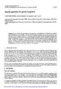
Figure 1: A dynamic junction tree of cliques. Any of the aforementioned three sections contains a set of random variables and a sub-graphical model over those random variables. The associated graphical model determines how the state space is structured: if the graph is a clique, then there is no inherent structure and the model might as well be an HMM. On the other hand, if the graph is very simple (like a chain or a tree of some sort) there are quite a large number of ways to produce efficient inference. Much more common is something between these two streams, and in such case, each of Gp , Gc , and Ge are triangulated [14] to form a junction tree [2] of cliques upon which a message passing algorithm [2] can be use used to perform probabilistic inference. In the dynamic case, however, the junction tree has a shape that looks something akin to Figure 1.

3. Search Methods in Speech Recognition Search methods in ASR have a long history [7, 18, 19]. The methods can for the most part be broken down into one of two approaches: synchronous vs. asynchronous.

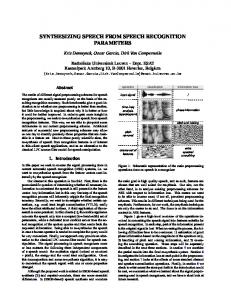
Figure 2: Left: asynchronous search. Right: synchronous search. Green depicts partially expanded hypotheses, red unexpanded portions of the space, and yellow continuation heuristics. In synchronous (also called Viterbi) search, hypotheses are expanded in temporal lock-step, where partial hypotheses that end at time t are expanded one at a time so that new partial hypotheses end at time t + 1. This then continues for all t so that at any given time there are never extant partial hypotheses with end-points at more than two successive time points. Asynchronous search, on the other hand, is such that the endpoint of partial hypotheses can have a wide variety. That is, each partial hypothesis ht has its own end-point consisting of a time-state pair, its own current score st , and it may be expanded without any temporal constraint. Asynchronous search is also called stack decoding, the reason being that one often keeps a priority-queue (implemented as a stack) of hypotheses and the hypotheses expansion occurs in a best-first order: the highest scoring hypothesis is expanded first. It is also useful in stackdecoding to have a form of continuation-heuristic (a value that estimates the score of continuing from the current point to the end of the utterance) so that the best-first decisions are based on the combined current hypothesis score and the continuation heuristic. If the continuation heuristic is optimistic (i.e., it is

an upper bound of the true score if the scores are probabilities), then the continuation heuristic is admissible and we have an A*-search procedure [6, 20]. Both synchronous and asynchronous search procedures have been used for speech recognition in the past, and the current prevailing wisdom is that synchronous procedures have for the most part bested their asynchronous brethren in popularity perhaps due to their overall efficiency, simplicity, and worderror performance [19]. One of the advantages of synchronous search is that beam-pruning is quite simple. Assuming that Mt is the maximum score of a set of states at time t, two simple widely used beam pruning strategies [21, 16] are as follows: with beam pruning, we remove all partial hypotheses that are some fraction below Mt , and with K-state pruning, (sometimes called histogram pruning ) only the top K states are allowed to proceed. K-state pruning is particularly attractive since it can be efficiently implemented using either a histogram [21], or by using a fast quick-sort like algorithm to select unsorted the top K out of N > K entries in an array. All need not lie in the extremes, however, as there can conceivably be hybrid approaches that straddle the fence between asynchronous and synchronous approaches. For example, a constraint can be placed on the maximum temporal distance between the end-point of any two partial hypotheses. Another approach would be to expand hypotheses based on some underlying (but constraining) data structure. In fact, this is something that a junction tree could easily do. Normally in a junction tree, the form of message passing is based either on the Hugin or the Shenoy-Schafer architectures [22]. Each of these approaches, however, assume that the cost of a single message is itself tractable, which is not the case in speech recognition due to the very large number of possible random variable values (e.g., consider the typical vocabulary size of a large vocabulary system). Therefore, even individual exact messages in a junction tree might be computationally infeasible and this is where the search methods from speech recognition apply. We consider the case where a search procedure is used to perform the junction tree message by expanding the clique. The expansion is constrained to apply only within the clique so that the decoding is “synchronous” but only at the clique level (we are not allowed to expand a clique Ct+1 until clique Ct has been expanded). Within a clique, however, the expansion can occur in any order, much like an asynchronous decoding procedure. However, since cliques can consist of any number of random variables, and could even span over short stretches of more than two time steps [14], then the cliques in the junction tree effectively limit the extent of the hypothesis expansion. By forming various triangulations (and corresponding junction trees) we can experiment with a wide variety of different search expansion constraints. We note that the two aforementioned pruning options can easily be extended to the junction tree case. Once a clique is expanded, we can compute the top scoring set of random variables in the clique, say it has score Mt . Then, any clique entries with score outside of the beam (using either beam pruning or K-state pruning) can be removed, and then the messages can proceed from there. Since the expansion can be asynchronous within a clique, moreover, it can be useful to establish a continuation heuristic so that only the most promising hypotheses are expanded (similar to a best-first search), but in this case, since we know that the expansion is limited to go no farther than the temporally latest variable within a clique, the continuation heuristic need not extend beyond a clique. On the other hand, since we are not

Our goal is to expand the hypotheses in the clique asynchronously. We also wish to prune while we are performing the clique expansion. For a given clique at time t, let Mt be the maximum score in the clique. The essential algorithm is to expand the hypothesis by considering the variables in a clique, and prune at the current point only if ˜t − b st + ct < M

(1)

where st is the score of the current hypothesis, ct is a contin˜ t is an estimate of the maximum score in uation heuristic, M the current clique, and b is the beam width. In practice, for ct , we use the maximum value possible continuation which ˜ t is exact. In normal search is an admissible heuristic if M methods, it would not typically be the case that it is possible to easily estimate Mt . With dynamic models, however, since similar repeated work has been performed for each past clique ˜ t . Assuming that {Cτ : τ < t}, we can reasonably compute M we have stored a history M1:t−1 of these maximum values, we may run a learning algorithm to produce a parametric estimate ˜ t = fθ (M1:t−1 ) of Mt . In practice we would use only a M fixed-length history, e.g., fθ (Mt−`:t−1 ). Once we have the real ˜ t . Important Mt we can correct θ given the error et = Mt − M in any estimate is that since this is running during decoding, it must be both very fast to compute and accurate. There is likely a tradeoff in that accuracy could be improved by spending more time in estimation. This procedure is the essence of online adaptive filtering [23], and it includes methods such as the well-known LMS and RLS algorithms, both linear models which are quite fast to compute and update but are often quite accurate. We therefore use these algorithms for doing our clique expansion pruning in our experimental section below.

5. Experiments We evaluate our approach on the 500 word task of the SVitchboard corpus [24]. SVitchboard is a subset of Switchboard-I that has been chosen to give a small and closed vocabulary. Standard procedures were used to train state-clustered withinword triphone models. A DBN with trigram language model [8] was used for decoding. As is well known, going from a bigram to a trigram will increase the state space of the model by a factor of the vocabularity size. The DBN for trigram decoding we used here is no exception. In this model, an additional word variable is added to explicitly keep track of the identity of the word that was most recently different. This additional word variable increases the complexity significantly. For this particular task, the state space of clique Ct is about 1011 . 5.1. Prediction performance of adaptive filtering The performance of predictive pruning greatly depends on how accurate the estimation of the maximum score is. In this subsection, we show the experiment results on evaluating the prediction performance of LMS filters. The relative prediction error rate Rt is used: Rt = 100

˜ t − Mt | |M . |Mt |

0 log probability

4. Predictive Pruning

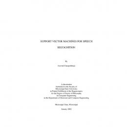
Figure 3 illustrates the true maximum scores along with the estimated maximum scores (using a 2nd order LMS filter with a learning rate of 1) on a particular Switchboard-I utterance. Notice that the true maximum score gradually and regularly decreases as time involves, making the prediction relatively easy. Indeed, the prediction is quite accurate as we can see from the figure.

true max score estimated max scoe

−2000 −4000 −6000 −8000

0

20

40

60 80 frame index

100

120

140

0

20

40

60 80 frame index

100

120

140

0 log10 relative error

expanding the model out to the last frame T (as is done in standard asynchronous decoding) to do this well, we would need to know Mt before we compute it. This chicken-and-egg problem, however, has a solution that suggests new approach to pruning based on online-prediction, as described in the next section.

−1 −2 −3

Figure 3: Comparison between the estimated maximum scores and the true maximum scores. We further evaluated the average prediction error rates (with prediction beam width 100) of different filters on the whole SVitchboard development set, along with the word error rates (WERs). In addition to comparing LMS filters with different orders and learning rates, we also compared LMS filters to a non-adaptive filter, i.e. a fixed 2nd-order filter defined as: ˜ t = 2Mt−1 − Mt−2 . The results are reported in Table 1. M Filter fixed LMS LMS LMS LMS LMS LMS LMS LMS LMS LMS LMS LMS

Order 2 2 2 2 3 3 3 5 5 5 8 8 8

Learning rate 0.01 0.1 1 0.01 0.1 1 0.01 0.1 1 0.01 0.1 1

Relative err. (%) 0.187929 0.206927 0.214376 0.289184 0.194498 0.201394 0.275253 0.173869 0.182693 0.252643 0.151899 0.161720 0.229042

WER(%) 46.7 46.7 46.8 47.4 46.7 46.7 47.4 46.8 46.7 47.3 46.8 46.7 47.3

Table 1: Prediction performance of adaptive filtering.

In general, with higher order, LMS filter performs better. Also, smaller learning rate seems to be preferred. In all cases, adaptive filters estimate the maximum scores near optimally – the average relative error rate is always within 0.3% across different parameter settings. Another observation is that, given small relative prediction error rates, all filters perform similarly in terms of WERs. 5.2. Comparison of pruning methods A good pruning algorithm should maintain a reasonable decoding accuracy while being faster, using less memory, or both.

59

beam pruning K state pruning percentage beam predictive pruning with LMS filter1 predictive pruning with LMS filter 2 prdictive pruning with RLS filter Probability mass pruning

57

WER(%)

55 53 51 49 47 45 0

5000

10000

15000

CPU time (seconds)

59 57 beam pruning WER(%)

55

K state pruning percentage beam

53

probability mass pruning predictive pruning with LMS filter 1

51

predictive pruning with LMS filter 2 49

predictive pruning with RLS filter

47

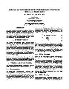
before, doing exact inference on this DBN is extremely expensive. At least 100G memory is required in order to get through all the utterances in our development set without any pruning. By doing beam pruning or K-state pruning, decoding is much faster, and at most only 2G of memory is used without hurting decoding performance (i.e., within 1% absolute difference of the WER of doing exact inference). Compared to beam pruning, K-state pruning makes the memory usage behavior more predictable and thus more controllable as one knows exactly an upper-bound on how many states the decoding will retain. As Gaussians were used in the model, the probability mass over the states can get quite concentrated on a small number of states. The consequence of such high concentration is that probability mass pruning either prunes off most of the states or does not prune at all. For instance, we observed that by keeping as much as (1 − 10−10 ) of the probability mass, probability mass pruning results in a WER over 70% since after each pruning step, fewer than 10 hypotheses survived. To mitigate this problem, we exponentiated the scores (only for the purposes of pruning), but while this retained more states, the non-linear distortions to the scores resulted in suboptimal performance. Compared to beam and K-state pruning, predictive pruning is significantly faster (upper plot in Figure 4) while using nearly identical memory (lower plot in Figure 4). As mentioned above, since predictions of the maximum scores are quite accurate for most of the filter setups, and since the additional computation due to the adaptive filter learning is negligible, predictive pruning with a 3rd order LMS filter performs similarly to a 5th order RLS filter, as shown in Figure 4.

6. References

45 7.8

8.3

8.8

9.3

9.8

log(acuumulated state space)

Figure 4: Learning curves of various pruning options. LMS filter 1 is a 2nd order LMS filter with learning rate 0.01. LMS filter 2 is a 3rd order LMS filter with learning rate 0.01. The RLS filter is a 5th order filter.

Therefore, we measured both memory usage and computation time of each pruning method on the SVitchboard development set. We use the accumulated clique state space of all the time frames of all utterances in the development set as an indication of memory usage. As for the speed measure, we performed all experiments three times independently on machines with Intel Xeon 2.33GHz CPUs, and the minimum CPU time of the three runs was used as the CPU time spent by that experiment. We compared the memory and time usage performances of various pruning methods including beam pruning, K-state pruning, percentage pruning, probability mass pruning (i.e. minimum divergence beam pruning [25]), and our proposed predictive pruning. Beam pruning and K-state pruning have been described in Section 3. Percentage pruning is a pruning method that retains top n% of clique entries with highest scores, while probability mass pruning retains clique entries that consist of the n% of the probability mass. Notice that all these pruning methods are performed after all the hypotheses of the clique has been expanded, while predictive pruning happens during the clique expansion process. Figure 4 shows the CPU time v.s. WER plot and state space usage v.s. WER plot for various pruning methods respectively. In general, both beam pruning and the K-state pruning perform reasonable well for the trigram decoding DBN. As mentioned

[1]

T. Cormen, Introduction to algorithms.

[2]

F. Jensen, An Introduction to Bayesian Networks.

[3]

P. Smyth, D. Heckerman, and M. Jordan, “Probabilistic independence networks for hidden Markov probability models,” Neural computation, vol. 9, no. 2, pp. 227–269, 1997.

[4]

X. Aubert, “An overview of decoding techniques for large vocabulary continuous speech recognition,” Computer Speech & Language, vol. 16, no. 1, pp. 89–114, 2002.

[5]

G. Saon, D. Povey, and G. Zweig, “Anatomy of an extremely fast LVCSR decoder,” in Ninth European Conference on Speech Communication and Technology, 2005.

[6]

D. B. Paul, “An efficient A* stack decoder algorithm for continuous speech recognition with a stochastic language model,” Proc. IEEE Intl. Conf. on Acoustics, Speech, and Signal Processing, 1992.

[7]

H. Ney and S. Ortmanns, “Dynamic programming search for continuous speech recognition,” IEEE Signal Processing Magazine, vol. 16, no. 5, pp. 64–83, 1999.

[8]

J. Bilmes and C. Bartels, “Graphical model architectures for speech recognition,” IEEE Signal Processing Magazine, vol. 22, no. 5, pp. 89–100, September 2005.

[9]

The MIT press, 2001. Springer, 1996.

T. Dean and K. Kanazawa, “Probabilistic temporal reasoning,” AAAI, pp. 524–528, 1988.

[10]

J. Lafferty, A. McCallum, and F. Pereira, “Conditional random fields: Probabilistic models for segmenting and labeling sequence data,” in Proc. 18th International Conf. on Machine Learning. Morgan Kaufmann, San Francisco, CA, 2001, pp. 282–289.

[11]

D. J. Rose, R. E. Tarjan, and G. S. Lueker, “Algorithmic aspects of vertex elimination on graphs,” SIAM Journal Computing, vol. 5, no. 2, pp. 266–282, 1976.

[12]

X. Boyen, N. Friedman, and D. Koller, “Discovering the hidden structure of complex dynamic systems,” 15th Conf. on Uncertainty in Artificial Intelligence, 1999.

[13]

K. Murphy, “Dynamic bayesian networks: Representation, inference and learning,” Ph.D. dissertation, U.C. Berkeley, Dept. of EECS, CS Division, 2002.

[14]

J. Bilmes and C. Bartels, “On triangulating dynamic graphical models,” in Uncertainty in Artificial Intelligence. Acapulco, Mexico: Morgan Kaufmann Publishers, 2003, pp. 47–56.

[15]

H. Ney, R. Haeb-Umbach, B. Tran, and M. Oerder, “Improvements in beam search for 10000-word continuous speechrecognition,” in 1992 IEEE International Conference on Acoustics, Speech, and Signal Processing, 1992. ICASSP-92., vol. 1, 1992.

[16]

S. Ortmanns and H. Ney, “Look-ahead techniques for fast beam search,” Computer Speech & Language, vol. 14, no. 1, pp. 15–32, 2000.

[17]

J. Bilmes and G. Zweig, “The graphical models toolkit: An open source software system for speech and time-series processing,” Proc. IEEE Intl. Conf. on Acoustics, Speech, and Signal Processing, 2002.

[18]

S. Young, “A review of large-vocabulary continuous-speech recognition,” IEEE Signal Processing Magazine, vol. 13, no. 5, pp. 45–56, September 1996.

[19]

X. Huang, A. Acero, and H.-W. Hon, Spoken Language Processing: A Guide to Theory, Algorithm, and System Development. Prentice Hall, 2001.

[20]

P. Gopalakrishnan and L. Bahl, “Fast match techniques,” Automatic Speech and Speaker Recognition (Advanced Topics), pp. 413–428, 1996.

[21]

V. Steinbiss, B. Tran, and H. Ney, “Improvements in beam search,” in Third International Conference on Spoken Language Processing, 1994.

[22]

A. Madsen and D. Nilsson, “Solving influence diagrams using HUGIN, Shafer-Shenoy and Lazy propagation,” in Uncertainty in Artificial Intelligence, vol. 17. Citeseer, 2001, pp. 337–345.

[23]

P. Clarkson, Optimal and adaptive signal processing.

[24]

S. King, C. Bartels, and J. Bilmes, “Svitchboard 1: Small vocabulary tasks from switchboard 1,” in Proc. Interspeech, Sep. 2005.

[25]

C. Pal, C. Sutton, and A. McCallum, “Sparse forward-backward using minimum divergence beams for fast training of conditional random fields,” in ICASSP 2006, 2006.

CRC, 1993.