Online Multiple Instance Joint Model for Visual Tracking

2012 IEEE Ninth International Conference on Advanced Video and Signal-Based Surveillance

Online Multiple Instance Joint Model for Visual Tracking Longyin Wen1 Zhaowei Cai1 Menglong Yang1 Zhen Lei1,2 Dong Yi1,2 Stan Z. Li1,2∗ 1 CBSR & NLPR, Institute of Automation, Chinese Academy of Sciences 2 China Research and Development Center for Internet of Thing {lywen,zwcai,mlyang,zlei,dyi,szli}@cbsr.ia.ac.cn

Abstract

acquire the features of the target by means of incremental PCA, which performs well in rigid or limited deformable motion because it constructs an adaptive appearance model of the target online. H. Grabner et al. proposed a discriminative model based on the online boosting [6], which has good performance in tracking because of its strong discriminative ability to recognize the target from the background. However, once drift problem happens, these generative and discriminative models cannot recover since they directly view their outputs as the positive sample for updating and the accumulated errors will finally result in their failure. To handle the drift problem, B.Babenko et al. proposed a robust discriminative tracker based on multiple instance learning [3]. The multiple instance mechanism ensures the tracker to extract the ’true’ samples for updating to alleviate drifting problem even when occlusion occurs.

Although numerous online learning strategies have been proposed to handle the appearance variation in visual tracking, the existing methods just perform well in certain cases since they lack effective appearance learning mechanism. In this paper, a joint model tracker (JMT) is presented, which consists of a generative model based on Multiple Subspaces and a discriminative model based on improved Multiple Instance Boosting (MIBoosting). The generative model utilizes a series of local constructed subspaces to update the Multiple Subspaces model and considers the energy dissipation of dimension reduction in updating step. The discriminative model adopts the Gaussian Mixture Model (GMM) to estimate the posterior probability of the likelihood function. These two parts supervise each other to update in multiple instance way which helps our tracker recover from drift. Extensive experiments on various databases validate the effectiveness of our proposed method over other state-of-the-art trackers.

Although the above methods perform well in some scenarios, it is relatively easy to lose the target because of the lack of mutual supervision system. Some researchers realized this problem and have developed several trackers with combined models. The trackers proposed in [21, 12, 13] combine several models with different views for tracking and adopt the co-training framework for updating. They achieve more stable performances than the single generative or discriminative tracker as the result of mutual supervision. In [17, 8], three models are incorporated in the tracker, which makes the tracker robust to certain situation. However, these trackers with combined models also suffer from drift problem and their updating samples are collected at the maximum posterior probability point with hard label (i.e. y = {−1, +1}), even when the confidences are low [7].

1. Introduction Visual tracking is one of the most fundamental and important problems in computer vision, and it has widely practical applications, such as human-computer interaction, video surveillance, robotics and etc. The tracker is required to capture the position and size of the target, but unfortunately, it is always influenced by many annoying factors, including occlusion, illumination variation and pose changes. Generative model [10, 16, 1, 11] and discriminative model [2, 3, 6, 18] are two major methods to address the above challenges. The generative model formulates the tracking task as a regression problem which searches the point with maximum likelihood. The discriminative model formulates the tracking task as a classification problem which focuses on the difference between the target and the background. Lim et al. proposed a generative model [10] to ∗ Stan

To deal with the problems existing in current trackers, we develop a novel joint model to accomplish the tracking task which is constituted by the Incremental Multiple Instance Multiple Subspaces Learning (IMIMSL) and the improved Multiple Instance Boosting (MIBoosting). The two parts supervise each other and they are updated in the multiple instance way. As discussed above, the mutual supervision system will provide our tracker more stability and the multiple instance updating strategy will help our tracker recover

Z. Li is the corresponding author

978-0-7695-4797-8/12 $26.00 © 2012 IEEE DOI 10.1109/AVSS.2012.52

319

from drift. Meanwhile, we assign the unlabeled data for updating with weights qualifying the probabilities of samples instead of the hard label, which will successfully avoid the manual threshold selection in hard label assignment and resist the noise more effectively. For the generative model that focuses on the target feature space, our proposed IMIMSL utilizes the subspace for updating, and the subspace is constructed by the representative weighted samples. To better acquire the target features, the energy dissipation of dimension reduction is taken into account in the updating step, which is always ignored in the previous proposed methods [10, 21]. For the discriminative model that concentrates on the difference between target and background, the improved MIBoosting is proposed. Different from the method in [3], we apply GMM to estimate the likelihood function p(f (x)|y = ±1), which can represent the practical probability of the likelihood function more precisely than the single Gaussian model.

the improved MIBoosting model extracts haar-like features [4]. In the following sections, the two parts of the joint model will be poured out in details.

3. Generative Model with Multiple Subspaces In the proposed multiple subspaces learning method, the packaged positive bags collected from the neighborhood of the tracker output are utilized for updating. The maximum probability instance within the bag is utilized to represent the bag for updating. The positive bag B is consisted by the instance set {I1 , · · · , In } and p(Ii ) is the probability of the ith instance within the bag to be positive, which is produced by the discriminative model. The weight of the maximum probability instance is calculated as: wI ∗ = p(B )p(I ∗ ), where I ∗ is the maximum likelihood instance and the Noisy-OR model is utilized nto estimate the probability of the bag, that is p(B ) = 1 − i=1 (1 − p(Ii )). Finally, the updating instance is selected in this way with the corresponding assigned weight.

2. Sequential Inference with Multiple Instance Supervision

3.1. Multiple Linear Subspaces Model

The tracking task is formulated as a state estimation problem and the motion process is assumed to be a Markovian state transition process. Let Zi = {z1 , · · · , zi } represent the observation data up to time i. xi is the state vector at time i, which contains the position and size of the target. In our tracker, the state vector is composed by X-axis, Yaxis, target width, target height. The posterior probability is estimated as the recursive equation:  p(xt |Zt ) ∝ p(zt |xt ) p(xt |xt−1 )p(xt−1 |Zt−1 )dxt−1 (1)

The appearance manifold of the target is highly nonlinear and it is hard for us to estimate it directly. However, multiple low dimension subspaces can be applied to approximate the manifold of the target. In this section, we propose a novel incremental learning strategy of the multiple local subspaces which utilizes the combined samples in adjacent frames rather than individual ones for updating. This learning strategy learns the features of the target more efficiently and reduces the homogeneous noise contained in the samples. Let M = {Ω1 , · · · , ΩL } represent the multiple subspaces of the target and Ωi , i ∈ {1, · · · , L} indicate the local subspace, where L is the total number of multiple subspaces. An observed instance z is a d-dimension image vector. Let Ωi = (μi , Vi , Λi , Wi , ni ), where μi , Vi , Λi ,Wi and ni represent the mean vector, the eigenvectors, the eigenvalues, the set of sample weights and the number of samples respectively. The multiple subspaces learning strategy is detailed in Algorithm 1. Approximate D representative instances are compressed into a local subspace. The subspace construction process can be completed by matrix SVD or the efficient EM algorithm proposed in [19]. A η-truncation is utilized to decide the reduction dimension of  the subspace  to maintain the en-

where p(zt |xt ) is the likelihood of the candidate samples. p(xt |xt−1 ) is the state transition probability and p(xt−1 |Zt−1 ) is the state estimation probability given all observations. Similar as [3], we adopt the simplest greedy Maximum a Posteriori Probability (MAP) strategy to solve the above equation, where the motion model is specified as p(xt |xt−1 ) = 1, if lt − lt−1  < r, otherwise p(xt |xt−1 ) = 0, where lt is the position of the target at time t, r is the search radius and the distance is the Euclidean distance. The appearance probability of the state xt is constituted by two parts, that is p(zt |xt ) = p(ztg |xt )p(ztd |xt ). The term p(ztg |xt ) is the probability produced by IMIMSL model and p(ztd |xt ) is given out by improved MIBoosting model. The two parts of the joint model select multiple updating samples for each other and the selected samples are packaged into bags for updating. Meanwhile, the noise is controlled efficiently by introducing the weights of updating samples instead of the hard positive or negative label, which are generated by the view’s counterpart. In our work, IMIMSL model utilizes the gray value of images as the feature and

ergy, that is q = arg mini



i λi tr(Λ)

≥ η . To evaluate the

probability of the sample, we utilize the maximum probability of the Lc nearest subspaces (Lc is set as 3 in the experiments). Set the observation variable of the IMIMSL model to be ztg and y t = (y1t , · · · , yqt ) = VtT (ztg − μt ), where t is the time index, Vt and μt are the eigenvectors and the eigenvalues of the subspace. The probability of the

320

Algorithm 1 Online Multiple Subspaces Learning Algorithm

Algorithm 2 The Subspace Updating Algorithm

Input: (‫ג‬, M, D, L) ‫{ = ג‬I1 , · · · , Ii , · · · }: a sequence of updating samples; M = ∅: the multiple subspaces; D: the number of samples for the updating subspace; L: the total number of subspaces. Set U to be the valid updating pool, symbol |U | represents the number of samples in the pool and k is the index of the updating sample. Output: M = (Ω1 , · · · , ΩL ): multi-local subspaces. while k ≤ |‫ |ג‬do if |U | < D then Add Ik to the updating pool U . else if There exists an empty subspace of M then Construct the subspace Ωn with the samples in pool U , Add Ωn to M and clear the updating pool U . else Construct the subspace Ωn by the samples in pool U , and calculate the similarity between subspaces, that is {p, q}∗ =  arg max Sim(Ωp , Ωq ), where  Ω p , Ωq ∈ {Ω1 , · · · , ΩL } {Ωn }, p = q. Ωm = Ωp Ωq , which means the subspace merging process, and replace the subspaces Ωp and Ωq with Ωm . Clear the updating pool U . end if end if k = k + 1. end while

1: Update the mean value of the subspaces, μ(k+l) = γμ(k) + (1 − γ)μ(l) , 

2:

instead of matrix LL .  Σ β , the size of matrix Q is (q + 1) × (q + 1), T β α   Σ1 A . Decompose Q as: Q = UΓU T , where Γ = where Σ = AT Σ2 1

diag{ξ1 , ξ2 , · · · , ξq+1 }, U T U = I . Then Vqk +ql +1 = LUΓ − 2 , where matrix Vqk +ql +1 = [v1,k+l , · · · , vqk +ql +1,k+l ] is composed by the first qk + ql + 1 eigenvectors of the covariance matrix S (k+l) .

4: The observation covariance matrix is represented as: S (k+l) = (ρσk2 + (1 − ρ)σl2 ) +

 

ωi ∈Wl

ωi2

2 ωi ∈Wk+l ωi

1

ωi ∈Wk+l

γ 2 ) 2 (μ(k) − μ(l) ) and γ =





ωi2

ωi ∈Wk

2

i λi,k+l k +ql +1 ξ j j=1

arg mini (  q

2

k+l

k+l

≥ η).

Furthermore, the covariance can be decomposed matrix qk T as the following Sk = σk2 I + i=1 (λi,k − σk2 )vi,k vi,k and  dk 1 2 we have the equation: σk = dk −qk qk +1 λi,k . We reformulate the equation above to get: (4) S (k+l) ≈ (ρσk2 + (1 − ρ)σl2 )I + LLT



2 ρ(λqk ,k − σk2 )vqk ,k where L = [ ρ(λ1,k − σ

k )v1,k , · · · ,

2 2 ρ¯(λ1,l − σl )v1,l , · · · , ρ¯(λql ,l − σl )vql ,l , y] and vi,k , λi,k , σk and vi,l λi,l , σl are the ith eigenvector, ith eigenvalue, energy dissipation in dimension reduction of the covariance matrix Sk and Sl respectively, and ρ=



ωi ∈Wk

ωi2

ωi ∈Wk+l

ωi2

, ρ¯ = 1 − ρ.

Considering the computation complexity, we decompose LT L instead of matrix LLT . Let Q = LT L. The size of matrix Q is q × q, where q = qk + ql + 1. Then the subspace updating process can be done efficiently by decomposing the matrix Q and the process is detailed in Algorithm 2. Specifically, when the updating subspace is constructed by only one individual sample, the proposed updating process is also applicable. In that condition, the covariance matrix S = 0, the mean value is equal to the feature value of the sample, and the reduction dimension equals 1. Please refer the supplementary material for more details about the deducing process of the subspace updating.

3.2. Performance Evaluation To verify the effectiveness of the model, we conduct a experiment in the sequences Sylvester and Minghsuan [10] with severe pose changes and challenging lighting respectively. Totally 4 subspaces are adopted in our model and we use the smallest projection error of 3 center nearest subspaces to be the measure. Every 3 frames are combined

(1 − γ)2 + ωi

ωi ∈Wk+l

T ξi vi,k+l vi,k+l . The first qk + ql + 1 eigenvalues

2

i

ωi2

i=1

(k+l) 2 ), where σ (k+l) = ρσk + (1 − ρ)σl2 , and qk+l = qk − ql − 1)σ 

where zi is the observations. We can get the covariance matrix of the merged subspace:   ωi2 ωi2 S (k+l) ≈  ωi ∈Wk 2 S (k) +  ωi ∈Wl 2 S (l) + yy T ωi ∈Wk+l ωi ωi ∈Wk+l ωi (3)  ωi ∈Wk

 qk +ql +1

of the covariance matrix can be updated as λi,k+l = σ (k+l) + ξi , and the  qk +ql +1 2 sigma value is updated as σk+l = d−q1 ( i=q +1 λi,k+l + (d −

The symbol ε(xi ) in the first item is the residual of the samples projected to the subspace, which is calculated as: ε(xi ) = xi − VV T xi . Subspace Similarity The similarity of the two subspaces is estimated as the weighted combination of the angle measure Simα (Ω1 , Ω2 ) and the compactness measure Simc (Ω1 , Ω2 ), which is defined as: Sim(Ω1 , Ω2 ) = Simα (Ω1 , Ω2 ) + ωSimc (Ω1 , Ω2 ), while ω is the trade-off between the two similarity measures and we set ω = 0.18 in our experiments. Please refer to [21] for more details. Subspace Updating The core problem in subspace incremental learning is the updating strategy. Our proposed strategy utilizes the subspaces for updating, namely merging the two most similar subspaces into one subspace. Derived from the basic equation of the maximum likelihood solution of traditional probability principal component analysis and taking the weights of the samples into account, the mean value μ(k) and covariance matrix S (k)  of the subspace are represented as: μ(k) =  1 ωi ωi ∈Wk ωi zi ωi ∈Wk  and S (k) =  1 ω2 ωi ∈Wk ωi2 (zi − μ(k) )(zi − μ(k) )T ,

where we set the relations: y = ( 



3: Set Q = LT L =

candidate sample to be positive is expressed [14] as:   q y t 2 2 (xi ) exp (− i=1 2λi i ) exp (− ε2σ 2 ) g √ p(zt |xt ) = (2) (2πσ 2 )(d−q)/2 (2π)q/2 Πqi=1 λi

ωi ∈Wk

ωi ∈Wk ωi . ωi ∈Wk+l ωi  2 ω ∈Wk ωi (k+l) Set ρ =  i ≈ 2 . Get the observation covariance matrix S ωi ∈Wk+l ωi 2 2 T T (ρσk + (1 − ρ)σl )I + LL . For simplicity, decompose the matrix L L T

where γ =

ωi .

321

Projection Error Curve of Sylvester 0.16

0.1

0.08

0.06

0.07

0.04

0.06 0.05

Multiple Instance Boosting is a learning method in which the training samples are not individually treated. The probability of a sample to be positive is  hi } (5) p(ztd |xt ) ∝ exp{

0.04 0.03 0.02

0.02

0

4. Discriminative Model with Improved Multiple Instance Boosting

IMIMSL (mean value:0.020) IVT (mean value:0.038) MLS (mean value:0.025) IPPCA (mean value:0.037)

0.08

Projection Error

0.12

Projection Error

Projection Error Curve of Minghsuan 0.09

IMIMSL (mean value:0.057) IVT (mean value:0.078) MLS (mean value:0.078) IPPCA (mean value:0.082)

0.14

0.01

0

100

200

300

Frame #

400

500

0

600

0

200

400

600

Frame #

800

1000

1200

Figure 1. The projection error curve of the our IMIMSL model and three other methods in two sequences.

i

Projection Error Curve with Different Parameters of Minghsuan 0.12

0.06

0.04

Paramemter:1−1−1 Paramemter:4−3−1 Paramemter:4−3−3

0.2

Projection Error

Projection Error

0.08

0.15

0.1

0.05

0.02

0

0.25

Paramemter:1−1−1 Paramemter:4−3−1 Paramemter:4−3−3

0.1

where ztd represents the observation of the improved MIBoosting model, and hi is the selected weak classifier. The training samples are packed into bags and the optimization objective is the bag rather than the individual samples. Compared with the conventional online boosting learning methods, the multiple instance boosting method is more robust to occlusion. Please refer to [3, 20] for more details. The key point in online boosting based methods is the way to update and estimate the weak classifier continuously after being given the samples. In the method proposed in [6, 3], the likelihood probability density function p(xj |y = 1) and p(xj |y = −1) are assumed to be the normal distribution which is not always true in practical, where xj is the j th dimension of the sample x . A more feasible way is to utilize the GMM instead of the single gaussian model to estimate the sample distribution p(xj |y = +1). According to the Bayesian rule, it is easy to get the continuous Bayesian weak regression function, p(x |y=+1) that is fj (x ) = log p(xjj |y=−1) with the assumption that the positive and negative samples have the equal probability in task, namely P (y = +1) = P (y = −1). When the weak classifier receives a positive bag with the samples {x (1) , x (2) , · · · , x (n) }, we calculate the mean value of the k th dimension, namely x¯k . Then the mean value is utilized to compute the probability of each Gaussian model in GMM and the Gaussian model which gives out the largest probability is the most matched one. Then the matched Gaussian model is updated with the received samples according to the method mentioned in [3], while the unmatched ones will not be updated. The corresponding weights of Gaussian model are updated as ω = (1 − λ)ω + λM , where M = 1 for the matched Gaussian model, M = 0 for the unmatched ones, and λ is the learning rate parameter which is set to be 0.2 in this paper. At the same time, the updating rules for the negative sample are similarly defined. Note that the form of weak classifier in our model remains the same as [3].

Projection Error Curve with Different Parameters of Sylvester

0

200

400

600

Frame #

800

1000

1200

0

0

100

200

300

Frame #

400

500

600

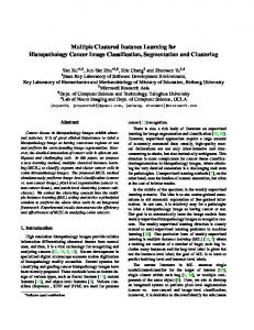
Figure 2. The projection error curve of our proposed method with dif-

ferent parameters of the test sequences. The symbol a-b-c represents the model has totally a subspaces and calculates the maximum probability of b-nearest subspaces, and every constructed subspace contains c combined samples.

to construct a new subspace for updating. The comparison is conducted with three other state-of-the-art learning strategies: IVT [10], the Multiple Linear Subspaces (MLS) model [21] and IPPCA [15]. The parameters of our model are fixed in these two sequences. The parameters of IVT, MLS and IPPCA are set as the default ones in their papers or codes. The comparison of projection error is shown in Figure 1. In both sequence, IVT and IPPCA have the worst performances, because they only construct a subspace which is updated with single sample. With the introduction of the multiple linear subspaces which are updated with combined samples, MLS outperforms IVT and IPPCA. However, its results are not as accurate as ours since our IMIMSL considers the energy dissipation of dimension reduction during the updating step. Furthermore, another experiment on the same sequences is conducted to find out the reason why our IMIMSL is effective. As seen in Figure 2, the model with the parameters 4-3-3 (blue line) obviously outperforms the other two models, while the model with parameters 4-3-1 (green line) has slightly better results than the one with the parameters 1-1-1 (red line). The minor difference between the green line and the red line indicates that the use of multiple subspaces will enhance the learning ability of IMIMSL, but it is not the main reason why IMIMSL has better performance than other learning methods. The significant improvement of blue line makes it clear that the multiple samples combination strategy greatly increases the performance of subspace learning methods, which is not pointed out in previous literatures.

5. Experiments We conduct some experiments to evaluate the performance of our joint model tracker. Our tracker is implemented in C++ code and runs at about 2 to 3 frames per second on the standard PC platform with 3.0GHz dual core CPU and 2GB memory without any optimization.

322

Experimental Setup The tracker is evaluated on 10 publicly available sequences which contains different challenging conditions. The sequences are issued in previous works: the sequences 1-3 from MIL[3], sequences 4-6 from VTD[9], sequences 7-8 from TLD[8] and sequences 9-10 from PROST[17]. Our tracker is initialized with the first frame and it outputs the trajectory of the target. The quantitative comparison results of IVT[10], FragTrack[1], SemiBoost[7], CoGD[21], MIL[3], PROST[17], VTD[9], TLD[8] and our tracker are shown in Figure 3, Table 1 and Table 2. More results can be found in the supplementary materials. Parameters The search radius of the tracker is set to [20, 50]. For the generative model, we set 4 subspaces to represent the target, and select 3 nearest of them to estimate the probability of the candidate samples. The updating samples are collected in the circle region with radius 4 and every 4 representative samples are combined together to update the multiple subspaces. For the discriminative model, 3 Gaussian models are utilized for the positive and negative sample, the number of candidate haar-like features is set as 300 and about 50 of them are chosen to construct the classifier. For the positive bags, the samples are collected from the circle with the radius 8 and about 35 of the collected samples are packaged in a bag according to the weight assigned to them. For the negative bags, 65 samples are collected from the ring with the radius interval [12, 40]. Moreover, we utilize the default parameters of other trackers which are public available and choose the best one of 5 runs, or take the results directly from the published papers. Specifically, we reproduce the CoGD tracker in C++ code and adopt the parameters as described in [21]. MIL Sequences The sequences tiger1 and occlude2 present frequent occlusions for several times. MIL and VTD have relatively better performance, because MIL adopts multiple instance updating strategy which is very robust to occlusion, and VTD efficiently combines some specific appearances of the target. Meanwhile, since the supervision strategy increases the possibility of our tracker to precisely find the target, our tracker also has the good performance, as supported by Table 1 and Table 2. The heavy 360◦ appearance variation and the occlusion by other similar object always challenge the stability of the trackers, just like what happens in sequence girl. While small drift exists, VTD and our tracker have the best performance. VTD Sequences There are numerous objects similar to the target in the background of the sequences animal, football and basketball. As seen in Figure 3, these similar objects always distract the detection based trackers away such as TLD and SemiBoost, because the appearances of the similar objects and the target are visually undistinguishable. Thanks to the supervision of the two different models in the multiple instance way, our tracker produces a little better

Seq. JMT IVT girl 10.9 40.4 occlude2 10.8 19.7 tiger1 8.01 80.7 animal 6.71 226 basketball 7.46 95.4 football 7.33 17.2 jumping 4.71 62.1 panda 5.68 58.2 lemming 12.5 128 board 25.3 169

CoGD Semi MIL Frag PROST VTD TLD 14.1 22.8 31.6 25.4 19.0 12.8 35.7 13.3 25.2 14.2 21.5 17.2 9.4 14.9 29.7 14.4 8.35 29.3 22.3 12.6 7.38 12.3 80.3 71.4 9.68 50.7 13.8 153 93.3 12.7 11 158 9.16 102 12.7 9.92 6.25 13.0 3.75 59.7 10.2 5.45 40.9 5.04 64.5 41.7 9.42 6.85 6.32 17.7 39.8 99.8 40.5 82.8 25.1 98 167 74.5 389 69.2 90.1 39.0 70.1 134

Table 1. Comparison results of average error center location in pixel. Seq. Frame JMT girl 502 492 occlude2 812 812 tiger1 354 265 animal 71 65 basketball 725 715 football 362 357 jumping 313 313 panda 1000 645 lemming 1336 1117 board 698 618

IVT CoGD Semi MIL 353 482 388 378 583 767 548 807 35 170 224 279 3 62 56 5 75 335 90 175 246 292 65 272 65 308 35 109 120 175 375 195 284 907 733 882 30 279 105 354

Frag PROST VTD TLD 378 447 502 219 618 665 792 712 155 189 150 13 66 43 630 601 15 302 357 272 258 79 209 465 510 315 733 942 471 234 474 524 274 95

Table 2. Tracking results. The total frame number of the sequences are presented in the second column. The number in other columns indicate the count of successful tracking frames based on the evaluation metric of PASCAL VOC object detection[5].

performance than VTD which is very good at dealing with this kind of challenges. TLD Sequences The sequence jumping contains abrupt motion because of handhold camera, and motion blur resulting from quick motion. These problems can be handled with an efficient appearance model or a detection module, such as FragTrack and TLD. Through combining a generative model and a discriminative model, CoGD and our tracker have more satisfactory results than other trackers. The frequent non-grid appearance variations in sequence panda result in less accuracy in tracking results, for example, IVT, CoGD and SemiBoost almost lose the target during tracking procedure. Since VTD incorporates several basic observation models and motion models into a compound tracker, it performs well in this sequence, but its tracking performance is still not as satisfactory as ours, as seen in Table 1 and Table 2. PROST Sequences The cluttered background in sequences lemming and board actually confuses the trackers a lot. Even the very stable tracker VTD easily loses the target, and TLD and SemiBoost based on detectors cannot successfully track the target for a long time, because the too much background information in bounding box leads to the failure of the detectors. Relatively, the trackers including CoGD, MIL and PROST which take the surroundings into account outperform other trackers including IVT and FragTrack which just consider appearance features. As illustrated in Figure 3, Table 1 and Table 2 experimentally, our tracker has the best performance because the joint model can effectively alleviate the influence of noise introduced by the complex background.

323

basketball 023

basketball 397

basketball 678

lemming 232

lemming 1110

lemming 1234

animal 012

animal 024

animal 059

football 113

football 285

football 307

board 071

board 574

board 671

tiger1 118

tiger1 223

tiger1 341

Figure 3. Tracking results. The results of our tracker, FragTrack[1], SemiBoost[7], CoGD[21], MIL[3], PROST[17], TLD[8] and VTD[9] are depicted as yellow, dark green, magenta, blue, black, light green, cyan and red rectangles respectively. Only the trackers with relatively better performances of each sequences are displayed.

6. Conclusion

[5] M. Everingham, L. J. V. Gool, C. K. I. Williams, J. M. Winn, and A. Zisserman. The pascal visual object classes (voc) challenge. International Journal of Computer Vision, 88(2):303–338, 2010. 5 [6] H. Grabner and H. Bischof. On-line boosting and vision. In CVPR, pages 260–267, 2006. 1, 4 [7] H. Grabner, C. Leistner, and H. Bischof. Semi-supervised on-line boosting for robust tracking. In ECCV, pages 234–247, 2008. 1, 5, 6 [8] Z. Kalal, J. Matas, and K. Mikolajczyk. P-N learning: Bootstrapping binary classifiers by structural constraints. In CVPR, pages 49–56, 2010. 1, 5, 6 [9] J. Kwon and K. M. Lee. Visual tracking decomposition. In CVPR, pages 1269–1276, 2010. 5, 6 [10] J. Lim, D. A. Ross, R.-S. Lin, and M.-H. Yang. Incremental learning for visual tracking. In NIPS, 2004. 1, 2, 3, 4, 5 [11] B. Liu, J. Huang, L. Yang, and C. A. Kulikowski. Robust tracking using local sparse appearance model and k-selection. In CVPR, pages 1313–1320, 2011. 1 [12] R. Liu, J. Cheng, and H. Lu. A robust boosting tracker with minimum error bound in a co-training framework. In ICCV, pages 1459–1466, 2009. 1 [13] H. Lu, Q. Zhou, D. Wang, and R. Xiang. A co-training framework for visual tracking with multiple instance learning. In FG, pages 539–544, 2011. 1 [14] B. Moghaddam and A. Pentland. Probabilistic visual learning for object representation. IEEE Trans. Pattern Anal. Mach. Intell., 19(7):696–710, 1997. 3 [15] H. T. Nguyen, Q. Ji, and A. W. M. Smeulders. Spatio-temporal context for robust multitarget tracking. IEEE Trans. Pattern Anal. Mach. Intell., 29(1):52–64, 2007. 4 [16] F. Porikli, O. Tuzel, and P. Meer. Covariance tracking using model update based on lie algebra. In CVPR, pages 728–735, 2006. 1 [17] J. Santner, C. Leistner, A. Saffari, T. Pock, and H. Bischof. PROST: Parallel robust online simple tracking. In CVPR, pages 723–730, 2010. 1, 5, 6 [18] F. Y. Shu Wang, Huchuan Lu and M.-H. Yang. Superpixel tracking. ICCV, 2011. 1 [19] M. Tipping and C. Bishop. Probabilistic principal component analysis. J. Royal Statistical Soc. Series B, 61(3):611–622, 1999. 2 [20] P. A. Viola, J. C. Platt, and C. Zhang. Multiple instance boosting for object detection. In NIPS, 2005. 4 [21] Q. Yu, T. B. Dinh, and G. G. Medioni. Online tracking and reacquisition using co-trained generative and discriminative trackers. In ECCV, pages 678–691, 2008. 1, 2, 3, 4, 5, 6

In this paper, a multiple instance joint model based robust tracker is proposed. The target appearance is constructed using the IMIMSL model that learns the appearance variations of the target and the improved MIBoosting model that differentiates the target from the background. The two parts of the model provide updating samples for each other and they are updated in the multiple instance way. Experimental comparison with the state-of-the-art tracking strategies demonstrates the superiority of our joint tracker. Our future work includes the introduction of the adaptive weight between the IMIMSL model and the improved MIBoosting model, which will provide our tracker more robustness.

Acknowledgement This work was supported by the Chinese National Natural Science Foundation Project #61070146, #61105023, #61103156, #61105037, National IoT R&D Project #2150510, Chinese Academy of Sciences Project No. KGZD-EW-102-2, European Union FP7 Project #257289 (TABULA RASA http://www.tabularasa-euproject.org), and AuthenMetric R&D Funds.

References [1] A. Adam, E. Rivlin, and I. Shimshoni. Robust fragments-based tracking using the integral histogram. In CVPR, pages 798–805, 2006. 1, 5, 6 [2] S. Avidan. Ensemble tracking. In CVPR, pages 494–501, 2005. 1 [3] B. Babenko, M.-H. Yang, and S. J. Belongie. Visual tracking with online multiple instance learning. In CVPR, pages 983–990, 2009. 1, 2, 4, 5, 6 [4] P. Doll´ar, Z. Tu, H. Tao, and S. Belongie. Feature mining for image classification. In CVPR, 2007. 2

324