IEEE International Symposium on Industrial Electronics (ISlE 2009) Seoul Olympic Parktel, Seoul, Korea July 5-8, 2009
Online Support Vector Regression based Value Function Approximation for Reinforcement Learning Dong-Hyun Lee!, Vo Van Quang'', Sungho J0 2 , Ju-Jang Lee 2 1 Robotics
Program, KAIST, Daejeon, Korea (E-mail:
[email protected]) 2School of Electrical Engineering and Computer Science, KAIST, Daejeon, Korea (E-mail:
[email protected]@
[email protected])
Abstract- This paper proposes the online Support Vector Regression (SVR) based value function approximation method for Reinforcement Learning (RL). This approach conserves the Support Vector Machine (SVM) 's good property, the generalization which is a key issue of function approximation. Online SVR can do incremental learning and automatically track variation of environment with time-varying characteristics. Using the online SVR, we can obtain the fast and good estimation of value function and achieve RL objective efficiently. Throughout simulation tests, the feasibility and usefulness of the proposed approach is demonstrated by comparison with SARSA and Q-Iearning. I. INTRODUCTION
By using RL, an autonomous agent that interacts with the environment can learn how to take a reasonable action for a specific situation [1]. Because of this merit, RL has been of interests not only in machine learning, but also in control engineering and other related fields [1], [2], [6]-[9]. RL provides a general methodology to solve complex uncertain sequential decision problems, which are very challenging in many real-world applications. The RL problem is, in many applications, modeled as a Markov Decision Process (MDP), which has been popularly studied [1], [2], [6]-[9]. An RL agent is assumed to learn the optimal or near-optimal policies from its experiences without knowing the parameters of the MDP. To find the optimal or near-optimal policy, a value function should be defined to specify the total reward an agent can expect at its current state. RL algorithms estimate the value function usually by observing data generated from interaction with the environment. Various value-function estimation techniques for RL have been proposed. The temporal difference (TD) algorithm suggested by Sutton [2] is one of popularly used techniques in these days. Especially finite-state MDPs have been approached throughout tabular method and tile coding or CMAC under the condition that states and actions are discrete. As for continuous state and discrete action problems, least square methods have proposed to estimate value functions using radial basis functions or kernels [7], [8]. For continuous state and action problems, gradient descent method and actorcritic network approach have been applied for value function
approximation [1], [9]. In this paper, we propose an algorithm to handle the problems with continuous states and discrete actions. Generalization property is an important factor to determine prediction performance with function approximation. SVM is known to have good properties over the generalization [5]. Therefore, applying SVR, which is the regression method of SVM, could be a good approach to estimate value functions. [6] proposes a method using SVR for state value function approximation used in RL. They use the TD error to apply SVR to RL. However, their approach is inattractive to solve online learning problem. Because it estimates a value function after visiting all states using the uniform random policy. In their approach, an RL agent can neither cumulate its experiences continuously nor adapt itself to the changing environment readily. An RL agent should generally be able to learn from data obtained sequentially from interaction with the environment. This paper proposes to use online SVR to more effectively and quickly approximate value functions used for RL. The idea about the online SVR is originated from the online SVM proposed by Cuwenberghs and Poggio [4]. The online SVR can be equivalent to approaches obtained by applying exact methods such as quadratic programming, However, the online SVR enables the incremental addition of new sample vectors and removal of existing sample vectors, and its process is quicker. A key idea of the online SVR consists in finding the appropriate Karush- Kuhn-Tucker (KKT) conditions for new or updated data by modifying their influences in the regression function while maintaining consistence in the KKT conditions for the rest of data used for learning. Our approach applies the TD error-based online SVR to estimate state-action value functions, which are directly used in RL. It does not require exact computation like quadratic programming. Therefore, computation load is low and learning speed is fast. An introduction to RL and online SVR is summarized in Section II, and our method is presented in Section III. In Section IV, some simulation results are shown to evaluate
449
978-1-4244-4349-9/09/$25.00 ©2009 IEEE Authorized licensed use limited to: Korea Advanced Institute of Science and Technology. Downloaded on April 07,2010 at 07:48:27 EDT from IEEE Xplore. Restrictions apply.
Statel Reward
Action
Environment Fig. I.
The agent-environment interaction in RL.
the performance of the proposed method. Section V draws conclusions.
II.
BACKGROUND
A. Reinforcement learning
As mentioned previously, a RL agent learns to find an optimal policy by interacting with the environment (Fig. I) The optimal policy is defined as follows [1].
7I"*(S)
= a rg
max Q(s, a)
aE A (s)
(1)
where s represents a state, a an action by the agent, A(s) a set of all possible actions, 7I"*(s) the optimal policy and Q(s,a) the state-action value function. If we know the state-action value function, we can easily find the optimal policy. But the state-action value function requires information on future rewards, so that it should generally be estimated. TD method is popularly used for the value function approximation. The method uses an error defined as follows [2].
r
+ "(Q(s', a') -
Q(s,a)
e-insensitive SVR problem is to find optimal values of weights w such that a parametric function f( x) = (w,x) + b can approximate output y within previously set error bound f . It can be formulated as follows [3] . min
l
l
(4)
0:;)
o < O:i, 0:; < C l
L(O:i - 0:;) = 0 where Q is the positive definite kernel matrix whose element is Qij = K( Xi , Xj) (K( ·, ·) is a kernel function). From partial deri vatives of W with respect to 0:, 0:*, and b, the following equations can be obtained.
D. oW
= 00: = ,
(3)
g* ,
subj ect to
~
oW
00:*
ob =
f (w , x 't·) + b - Y·'l. < _
L
l
j
Qij (3j - Yi + I'
+b
l
,
oW
I'
where i = 1, ... l, i is the number of training data, b represents the bias term, and the constant C > 0 determines the tradeoff between the flatness of f (x) and the amount up to which deviations larger than I' are tolerated [3].
i
l
subject to
i= l
Yz· - (w , x 1.·) - b _
0
I
"2 llwl12+ C 2)~i + ~n
and 9~
>0
Re move c fro m R a nd ex it
I
Dec rement Pc. upd ati ng Pi for i E S and 9i. 9i for i ct S unt il one of the fo llowing co nditions holds: [9c ::; 0 ? )---- - Pc = 0: Rem ove c from R and ex it - One vector migrates from/to sets E. E ' or R to/from S : update set memb erships and update lR Incremen t Pc. updati ng Pi for i E S and 9i. 9i for i ct S until one of the follow ing co nd itio ns holds: [ 9~ ::; 0 ?)---- - Pc = 0: Rem ove e to R and exit - O ne vect or migrates fro m/to sets E . E' or R to/f rom S: upd ate set membe rship s and upd ate lR
Fig. 3.
We propose to use onli ne SVR to provide the state -action value function approximation to RL. App lications of online SVR so far have used output approximation error to find optimal weights, but we propose to use the TD error. Therefore, our onli ne SVR aims to find optimal weights to make the TD error less than the allowed maxim um devia tion E. In our method, the state-action value function is approximately set to Q( s ,a) = wT¢(s ,a) + b where ¢ (s , a ) is the feature vector (radial basis functio ns can be chosen as the feature for example). With this approximation, the problem formulation is modified from (3) as follows . min
19c:S 0 ? ~
Increment Pc. updatin g Pi for i E S and 9i. 9i for i ct S until one of the follow ing condit ions holds: - 9c = 0: add c to S. update lR and ex it - Pc = C: add e to E and exit - One vector migrates from/t o sets E . E ' or R to/from S: upd ate set member ships and update lR
SVR TO RL
1
Add c to R and exit ]
(6)
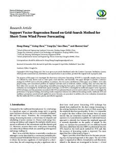
A new vector c is added by inspecting ge and g~ . If both values are positive, c is added as a R vector because that means that the new vector lays inside the e-tube and it does not affect on the existing data in D. When ge or g~ are negative, a new vector is added by setti ng its initial influence on the regression (f3e) to O. Then this value is carefully modified (incremented when ge < 0 or decremented when s; < 0) until its ge, s; and f3e values become consistent with respect to the KKT conditions (that is, ge < 0 and f3e = C, or g~ < 0 and f3e = - C , or 0 < f3e < C and ge = 0, or - C < f3e < 0 and g~ = 0 ). Fig .3 (a) shows the whole process of adding new vector. ~ in the algorithm is a matrix to be maintained and upda ted to calculate the f3;'s (see equations (12) and (13)) . The proce dure for removing vector from the data set uses the similar principles for adding new vector as in Fig . 3 (b) . The detai ls can be found in [5].
III.
(a)
I
Procedure for (a) adding and (b) removing a vector.
Then, the corresponding cost function is as follows . W
1
= "2
(a - a *fVVT(a - o ") +
I E
L ) ai
+
an
i= 1
I
- L
ri (ai -
i =1
an + (1 - 1')b L
I
(a i -
i= 1
an
(9)
subject to
o < a i , a; < C I
(7)
L
i= 1
subject to
(a i -
an = 0
where Q( Si' ai) ~ E + ~i A " A * - r i - I'Q (Si' a i) + Q(Si ' ai) ~ E + ~i
ri
+ I'Q (s~ , a~) -
By applying the definition of rewritten to be :
Q,
V ij
= l'¢j ( s~, aD
- ¢j (Si' ai)
From (9), new gradient functions can be obtained as follows.
= V iVT f3 + E - ri + (1 - 1')b gi = - V iV T f3 + E + r i - (1 - 1')b =
the constraints can be
gi
- gi
+ 2E
(10)
The main difference between (5) and (10) is that Yi and b is rep laced by r i and (1 - 1')b respectively. When a new vector 451
Authorized licensed use limited to: Korea Advanced Institute of Science and Technology. Downloaded on April 07,2010 at 07:48:27 EDT from IEEE Xplore. Restrictions apply.
0. 1
with influence (3c is added, the variation in gi, gi , and (3i can be calculated by (11) without migration of vectors between sets S, E, E * and R.
6gi = Qic6 (3c + L Qij6(3j j ES 6g7
=
+ (1 -
0.1
(II)
=0
Fig. 4.
Because 6g i = 0 for i E S, the influence of the new vector can be calculated by the following equations.
4-slale chain walk problem (this figure is adapted from [7]).
5 r----,-----,-----,
..: 3 · ·
0'
.;
00
~~l;
1
QS1,Sl
QS1,Sl
QSl ,Sl
QSl,Sl
The influence of the new vector for i by the following equations.
6g i
=
Qic6 (3c + L Qij6(3j j ES
(Q ic + L Qij c5j j ES 6(3c = 1'i
=
r
I
L i= l
(3d1'¢( xD - ¢ (Xi)) ¢ (x ) + b
.
00
100
200
300
No. of state movements
No. of state movements
5 r----,-----,-----,
5 r----,----,-----,
4
4 ..
., .
, .
300
No. of state movements
(14)
No. of state movements
IV. SIMULATION
= w T ¢ (x ) + b =-
300
:
} I.....:..':.-:-:::-.:: :-::::.-:- -
Fig. 5. State-action value function estimate for 4-state chain walk (the solid line indicates Q (s, R), the dashed line indicates Q (s , L)) .
Equations (12) and (14) are valid while vectors do not migrate from set S, E, E *and R to another one . But in order to satisfy KKT conditions consistently for the new vector c, it could be necessary to change first the membership of some vectors to these sets or to update matrix ?R in some cases. (3c is modified incrementally or decrementally until one migration is forced. If the migration occurrs, membership change for the data should be executed, and then the variation of (3c continues. The whole process of adding new vector or removing existing vector is according to Fig. 3. Online SVR can be trained from sequentially added data using this algorithm and the approximated state-action value function can be calculated to be:
Q( x)
200
~ ~ ~~ .. .I.~.~ ~
1')6 b
+ c5)6(3c
100
, ..
5 r----:-----,----,
(13)
'f- S can be calculated + (1 -
'~ i'-::';~"-""""'''''''''';'''''''''''''''''~
2 1j.·· ~:~ ,, ~ ~ :~ ~ ~ ~ 1
1
0.1
0.1
~
where
0.1
1')6 b
- 6 9i
6 (3c + L 6 (3j j ES
0.1
(15)
We apply proposed method to two problems. The first one is the 4-state chain walk problem, which is a simple toy problem introduced in [7] . The other one is cart pole balancing problem, which has been popularly used for algorithm evaluation [I] , [7]. In both cases , the state-action value function is estimated by the proposed method. A. 4-state Chain Walk
Fig. 4 shows the 4-state chain walk. There are 2 actions available (L: going to the left and R: going to the right) and 4 states . The rewards over states are 0, + I, + I, and 0 respectively. If one action is selected, the agent takes that action with probability 0.9 and the other with probability 0.1. Radial basis kernel is used to estimate the state-action value function. The optimal policy of this problem is (R, R, L, L). In Fig . 5 the state -action values are depicted . The solid line represents the state-action value for action R and the dashed represents that for action L. We can see the state-action values converges eventually after 128 state movements in Fig. 5.
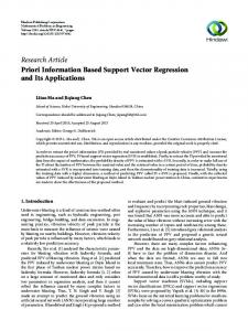
B. Cart-Pole Balancing Problem where x represents a new state-action pair and x~ and Xi means the next state-action pair and current state-action pair of i1h sample respectively.
Fig. 6 shows the cart-pole balancing system. An agent applies forces to the cart in appropriate directions to maintain the pole's upright position on the cart. There are two actions: pushing the cart to the left with force f = - ION and to the
452
Authorized licensed use limited to: Korea Advanced Institute of Science and Technology. Downloaded on April 07,2010 at 07:48:27 EDT from IEEE Xplore. Restrictions apply.
(a) ·4
·2 30JJ r--'---;----'-----.,.--'---;---........:.---j
Fig. 6.
Cart-pole Balancing System.
······ r - ;"+-'-;;..'_·.i·-h< :·.:.::i: :.:.::.:.::.:.: ..:.: ::::::.:.·::..:.:·.:
2500
TABLE I
*:mJ ,..
I:
(J)
PARAM ET ERS FOR THE DO UBL E PO LE BALA NCI NG PROB LEM
~.~ ~ . . .
·
R
•••••• ,
0)
c:
Symbol
Description
Value
x
Position of cart on track
[-2.4, 2.4] m
(J
Angle of pole from vertical
[-45, 45] deg.
f
Force applied to cart
-10 N or 10 N
I
Half length of pole
1 =0.5m
M
Mass of cart
1.0k g
m
Mass of pole
O.lkg
'u c:
1500
'"
0;
co
..
..,
.
,,
100) I
500
i, ,_r- _ _ ~ - -L -L o,...'====-'''-====='-='-==-='''-"-'='--'''-'--=-.1._ --'-- ' -- ' ----'' o 50 100 150 200 250 300 350 400 450 500 I
No. of episodes
(b)
right with f = ION. The dynamics of the system is described in (16), but unknown to the agent. Table I describes variables and parameters.
e
=
(gsine - Fcose) j
(~l -
r
,
c
,
,.-------'----.._--'---___,_---;
2500 r ····...; ········:-· ······· ,······· I
mlcos 2e j(M + m))
= F - mlecose j(M + m) F = (J + mliP si n e )j(M + m)
i
30JJ
(16)
4 states (cart position, cart velocity, pole angle, and pole angular velocity) are used to train the online SVR. Radial basis kernel is used to estimate to the state-action value function. If the cart position is less than -2.4 m or greater than 2.4 m, the system returns reward -1. Also, if the angle of pole is less than -45 deg or greater than 45 deg, it also returns -1. In the other states, the reward is 0. If the reward is -1, that episode terminates and a new episode starts. The initial state is (0, 0, 0, 0). We assume that the task is successfully achieved if the cart-pole system still maintains balancing in 3000 steps. The simulation results of online SVR based RL are depicted in Fig. 7 (a). To evaluate the performanc e, the results of applying SARSA and Q-Iearning for the same problem are presented in Fig. 7 (b) and (c) respectively. In SARSA and Q-Iearning, tabular method is used to estimate state-action values. There are 324 state-action values ( 3 cart positions x 3 cart velocities x 6 pole angles x 3 pole angular velocities x 2 actions). Fig. 7 (a) to (c) depicts the best, the worst, and the average performance of each method. we can see the proposed online SVR based RL learns and finds an optimal policy much more quickly than SARSA and Q-Iearning. In the best performance case, SARSA achieves the task successfully after 200 episodes and Q-Iearning does after 170 episodes. But, online SVR based RL succeeds the task after 3 episodes only. In both SARSA and Q-Iearning, the tabular method cannot estimate stateaction values properly until the states are visited. Furthermore, it affects negatively for RL agents to estimate other state-action
5OOr··· ···'. ·· 1I
200
250
300
350
400
450
500
No. of episodes
(e) 30JJ ~
;
c
,
,.----'-rr""T"i"-
-'--
-;--
'--........:.-
--j