Online Terrain Classification For Mobile Robots Edmond M. DuPont†, Carl A. Moore‡, Majura F. Selekwa‡, Rodney G. Roberts†, Emmanuel G. Collins‡ Department of Electrical and Computer Engineering†, Department of Mechanical Engineering‡ FAMU-FSU College of Engineering Tallahassee, FL 32310, USA
[email protected]
Abstract— Todays unmanned ground vehicles (UGV) must operate in and increasingly general set of circumstances. These UGV’s must be able to provide stable controlability on whatever terrain they may encounter. A UGV might begin a assignment on asphalt but quickly be required to negotiate sand, mud, or even snow. Traversing these terrains can affect the performance and controllability of the vehicle. Like a human driver who can feel his vehicles response to the terrain and make changes to compensate, a UGV that could autonomously determine the current terrain type could also make necessary changes to its control strategy. This article focuses on the development and application of a terrain detection technique based on terrain induced vehicle vibration. Using IRobots ATRV Jr mobile robot equipped with various sensors, we extract the frequencies of the vehicles terrain induced vertical acceleration. These frequencies are input to a fast online terrain classification algorithm based on the Probabilistic Neural Network. We present terrain classification results for the robot traveling at various speeds over multidifferentiated terrains broadly classified as sand, grass, asphalt, and gravel.Todays unmanned ground vehicles (UGV) must operate in and increasingly general set of circumstances. These UGV’s must be able to provide stable controlability on whatever terrain they may encounter. A UGV might begin a assignment on asphalt but quickly be required to negotiate sand, mud, or even snow. Traversing these terrains can affect the performance and controllability of the vehicle. Like a human driver who can feel his vehicles response to the terrain and make changes to compensate, a UGV that could autonomously determine the current terrain type could also make necessary changes to its control strategy. This article focuses on the development and application of a terrain detection technique based on terrain induced vehicle vibration. Using IRobots ATRV Jr mobile robot equipped with various sensors, we extract the frequencies of the vehicles terrain induced vertical acceleration. These frequencies are input to a fast online terrain classification algorithm based on the Probabilistic Neural Network. We present terrain classification results for the robot traveling at various speeds over multidifferentiated terrains broadly classified as sand, grass, asphalt, and gravel.
INTRODUCTION Field applications of unmanned ground vehicles require these vehicles to traverse a wide variety of terrain types, including asphalt, gravel, sand, mud or any combination thereof. Since different terrains require different forms of maneuvering control, there is a growing a interest in online terrain detection capabilities for unmanned ground vehicles that are to be used field operations. Most proposed methods for terrain detection have been based on machine vision, whose accuracy depends on the light intensity. Howard and
Seraji introduced the Fuzzy Traversability Index algorithm which uses visual intensity levels to determine the terrain characteristics such as the roughness, slope, and discontinuity [1]. These characteristics are used to determine whether the terrain is traversable prior to crossing. This approach becomes unreliable in situations where the variation in the light intensity between the terrain and obstacles is uniform such as in low ambient conditions. Some of the methods that avoid the effects of variability in light intensity use statistical properties of 3D ladar data to detect the surrounding environment. These methods can be computationally expensive, and they are limited to discriminating between vegetation and solid surfaces such rocks [2]. In general, ladar based methods use image processing and statistical analysis to classify a scene into surface classes such as grassy or ground. In most cases these are offline methods. An efficient method for online terrain classification is based on an analysis of the interaction between the vehicle and the terrain. In these methods terrain classification is treated as a signal processing problem in which the terrain is modeled using parameters that can be determined directly from UGV sensor data produced by the interaction between the terrain and the vehicle. An algorithm based on terrain interaction may compliment the vision based algorithms mentioned above by enabling the robot to sense its terrain by both ”feeling” and ”seeing” it not unlike how humans determine the terrain on which their cars are driving. Exploring the ability to determine a terrain through feeling, Iagnemma et. al. characterized a terrain by its cohesion and internal friction [3], [4] while internal sensors measured the vertical load, torque, wheel sinkage, wheel angular speed, and wheel linear speed. These measurements were used in simplified forms of classical terramechanics equations to compute terrain parameters which were compared to stored parameters of known terrains. Since the equations on which the method is based require the wheels to be in contact with the ground, this method may not be attractive for some UGV field applications. There have been efforts to improve it for use on high speed vehicles by combining it with visionbased classification along with the ground-wheel vibration signature classification [5]. This paper presents a method that characterizes terrain entirely by the frequency response of the vehicle. It assumes that the vehicle vibration depends on the terrain and has
a unique frequency response signature which is a function of the terrain type. The typical set of frequency response data previously taken from each terrain type is statistically compared to the measured frequency response data using a probabilistic neural network; a match between the two sets is used to estimate the current terrain. The frequency response approach, which was first suggested in [5] and initially presented in [6], [7], treated the vehicle as a particle with only one degree of freedom. The classification was carried out statistically using a probabilistic neural network. Similar results were recently published by Brooks where the classification was carried out using principle component analysis [8]. Treating the vehicle as a particle results in poor performance at certain speeds and on certain terrains, especially when vibration amplitudes are low or out of phase. The method presented in this paper models the vehicle as rigid body with at least three degrees of freedom. The classification is carried out statistically using a probabilistic neural network [6], [7]. The paper is divided into six sections. Section I describes the platform vehicle and presents a justification for why a vehicle model built with three degrees of freedom yields better results than one degree of freedom models [6], [7], [8]. Section II describes how the vehicle vibration data is collected and processed to extract the required terrain features. Statistical processing of the extracted terrain features and eventual detection of the terrain is described in Section III. The field tests results obtained using the proposed method are presented and discussed in Section IV. The paper presents concluding remarks in Section V.
velocities of the vehicle about the vehicle’s main axes. This
Fig. 2. Crossbow DMU sensor for measuring gyro rates and accelerations along the vehicle’s principal axes
z
Vehicle y
x
Suspension
Terrain
Wheel Tyre
I. T HE TARGET UGV P LATFORM AND T ERRAIN M ODEL The target UGV platform for the results presented in this paper is iRobot’s All Terrain vehicle (ATRV-Jr) shown in Fig. 1. This is a skid steered mobile robot weighing approx-
Fig. 3.
Vehicle Model: A vibrating system with base excitation
vehicle can be modeled as a vibrating system with base excitation as illustrated in Fig. 3. In general, the terrain is an irregular surface with random height g(x, y, ω) at position x, y that can be modeled as [9]: Z x Z y g(x, y, ω) = Q(x−u, y−v)h² (u, v, ω)dudv. (1) −∞
Fig. 1.
iRobot ATRV-Jr Robot Platform
imately 50 Kg and with a maximum speed of 1.4 m/sec. The particular vehicle used in these experiments is equipped with an onboard computer powered by a Pentium 3 800MHz processor running the Linux 7.2 operating system. Various sensors are mounted on the ATRV-Jr; the most important for the purpose of this paper is the differential measurement unit (DMU). The DMU is mounted within the body of the robot underneath the onboard computer, as shown in Fig. 2; it measures the translational accelerations and rotational
−∞
The function Q(·, ·) is terrain dependent while h² (·, ·, ω) is a weakly stationary and weakly correlated random function of frequency ω. Hence the vehicle is randomly excited by the terrain at the four wheels. Each wheel vibrates with a profile approximated by gw (x, y, ω), gw (x, y, ω) = m(x, y, ω) ± d(x, y, ω)
(2)
where m(x, y, ω) is the mean value of wheel vibrations and d(x, y, ω) is the difference in vibrations of the wheel from the mean value. If the wheel vibrations were available, then the terrain could be estimated by using the mean vibrations of the vehicle wheels and their differences. However, quite often the wheel vibrations are difficult to measure accurately. Instead the vibration of the vehicle as a single body is measured using the DMU sensor [10], [11].
FFT of Z axis Acceleration
II. F EATURE E XTRACTION
The classification task is essentially a mapping problem where we attempt to determine the best fit for x in a region of vector space (terrain space) as illustrated in Fig. 7. We use an artificial neural network called the probabilistic neural network (PNN) to perform the mapping. The PNN is introduced in the next section.
Normailzed Magnitude
Gravel Grass Asphalt
0.35 0.3 0.25 0.2 0.15 0.1 0.05 0
4
6
8
10
12
Frequency (freq) Fig. 4. Z-axis acceleration frequency response of the vehicle while traveling over gravel, grass, and asphalt
Normailzed Magnitude
FFT of Roll Velocity Gravel Grass Asphalt
0.35 0.3 0.25 0.2 0.15 0.1 0.05 0
4
6
8
10
12
Frequency (freq) Fig. 5. Vibration frequency of the vehicle about the X-axis while traveling over gravel, grass, and asphalt
FFT of Pitch Velocity
Normailzed Magnitude
The problem of terrain identification for robotic vehicles can be viewed in some aspect as a pattern classification problem in which the pattern is the terrain induced vehicle vibration. Pertinent features of the terrain are extracted from the vibration signals in a way that reduces the dimension of the classification patterns while providing high classification accuracy; these features serve as the terrain signatures. The inclusion of an increased amount of features can lead to degradation in classification performance especially when features that do not change significantly with terrain changes are included. Therefore, only features that have discernable changes as a function of terrain type should be used. The features used in this work are based on the structural characteristics of the frequency components of a time signal. Specifically, the time signal is a combination of the vehicle’s linear and angular vibrations as measured using the robots DMU sensor, and we extract its frequency components using the Fast Fourier Transform (FFT). As the robot traverses various terrains our DMU sensor measures the vehicles linear accelerations along the three body fixed axes and the angular velocities about these axes. We consider these six values to the represent the vehicles complete vibration signature. However, since one of the angular velocities, ωz , about the robots vertical axis (zaxis), and two of the linear accelerations x ¨ and y¨, along the longitudinal and transverse axes respectively, are highly correlated with the robot’s changing speed and heading, we chose to model terrains as a function of the remaining three vibrations: the linear z-axis acceleration and the angular velocities about the x and y axes, i.e.: z¨, ωx , and ωy respectively. These measurements can be influenced by the contour of the surface, as when one side of the robot has a higher elevation than the other, but in the experiments presented herein the robot followed a path along a globally flat surface. The typical FFT results for the linear and angular vibrations of the vehicle are shown respectively in Figures 4, 5, and 6. We found that different terrains at a given speed produced significant and consistent magnitudes of acceleration along the z-axis within the frequency range of 3 Hz through 25 Hz. Somewhat less dominant are the vibrations about the x and y-axes in figures 5 and 6. After several experiments, it was confirmed that terrain signatures can be extracted from the frequency components of the vibrations along the z axis and about the x and y axes. Therefore, we defined a terrain ”feature vector” x with these three components fz¨, fωx and fωy corresponding to the dominant reactions of the vehicle to a terrain: £ ¤T x = fz¨, fωx , fωy (3)
0.4
Gravel Grass Asphalt
0.35 0.3 0.25 0.2 0.15 0.1 0.05 0
4
6
8
10
12
Frequency (freq) Fig. 6. Vibration frequency of the vehicle about the Y -axis while traveling over gravel, grass, and asphalt
III. T HE F EATURE M APPING P ROCEDURE This section describes how a PNN was used to classify the feature vector x as a particular terrain. Several tools such as the backpropagation multilayer perceptron, support vector machines, and other similar methods for pattern classification could have been used [12], [13]; however, we chose the PNN because of its simplicity, robustness to noise [14], and fast training speed.
fy Terrain 1 Terrain 2
Feature points (x)
fx
Terrain 3 fz
Fig. 7.
Terrain determination analogy in a vector space
A. Probabilistic Neural Networks The PNN [14], [15] is a pattern classification network that is based on the classical Bayes optimal classifier. Recall that the Bayes decision rule states that an unknown vector x is assigned to class ci of a two category case: hi li pi (x) > hj lj pj (x),
i 6= j
(4)
where hn is the prior probability of occurrence, ln is the loss associated with misclassifying an object to class n, and pn (x) is the probability density function (pdf) of class n. The PNN simplifies this decision rule by assuming that the prior probability hn and the loss function ln are equal for all categories; therefore, the decision is based entirely on the probability density function, which reduces (4) to: pi (x) > pj (x),
∀i 6= j
φ(·) is the window function, and hn is the window width [16], [17], [18], [19]. Normally, the Gaussian distribution is used as the window function φ(·) and (8) becomes: " # nti X (x − xij )T (x − xij ) 1 P (ci |x) = exp − N 2σ 2 (2π) 2 σ N nti j=1 (9) where xij is the j-th sample data point for the patterns in class i, σ is known as a smoothing factor corresponding to the volume contained in the sample data points, N is the dimension of the vector corresponding to the data point, and nti is the number of sample patterns in class i. The smoothing factor σ can vary between 0.1 and 10; for nonlinear decision boundaries, the smoothing factor needs to be as small as possible. In this work, the shape of the decision boundary was assumed to be nonlinear; hence, a smoothing factor σ = 0.15 was found to yield acceptable classification results. The network structure of the PNN is shown in Fig. 8. The network has an input layer, a pattern layer, a summation layer, and an output layer. The input layer simply buffers all the inputs x to the pattern layer with one neuron for each feature vector. For each neuron in the pattern layer a weighted sum of the testing feature vectors from the input layer is calculated. The weights of each of these neurons are set to the training feature vectors. The nonlinear activation INPUT FEATURE VECTOR (x)
f
y
f
z
Feature Patterns for Terrain m
Feature Patterns for Terrain 1
(5) PATTERN LAYER
f1(x)
(7)
The conditional probability P (ci |x) is eventually estimated by using the Parzen window method, which superimposes window functions centered at the sample data points as µ ¶ n 1X 1 x − xi P (ci |x) = φ (8) n i=1 Vn h where n is the number of sample data points, Vn is the volume of the region under which the n sample points fall,
f2(x)
fm(x) SUMMATION LAYER
OUTPUT LAYER
(6)
where P (x|ci ) is the conditioned probability density function of x given set ci , and P (cj ) is the probability of drawing data from class cj . Now, the vector x is said to belong to a particular class ci if: P (ci |x) > P (cj |x), ∀j = 1, 2, · · · , n, j 6= i
f
INPUT LAYER
It is a known limitation of (5) that the pdf of x for all classes is not known, meaning (5) can not be directly implemented. The PNN avoids this problem by using the Bayes conditional probability rule P (ci |x) of vector x being in class ci : P (x|ci )P (ci ) P (ci |x) = Pn j=1 P (x|cj )P (cj )
x
Output class for the given input vector
Fig. 8.
Architectural Structure of Probabilistic Neural Network
function (9) is applied to the calculated weighted sum and is fed as the neuron’s output to the summation layer. The weights on the summation layer are fixed to 1 to allow equal probability for all terrains, in which the outputs of the pattern layer are added together. In general the summation layer computes the probability fi (x) of the given input x belonging to the class i represented by the patterns in the pattern layer. The output layer picks the class for which the highest probability was obtained in the summation layer. The effectiveness of the network in classifying input vectors depends highly on how the training patterns are chosen. One advantage of applying the PNN is, given its parallel architecture, it exhibits fast calculations for training and
testing, which becomes beneficial for online processes. Its speed derives from the fact that the network is essentially a one pass feed-forward network where the network weights are assigned as the training data. In addition, for a timevarying statistical analysis, training patterns can be increased or older training patterns can be overwritten by new patterns. A disadvantage of the network is that the computational expense is proportional to the dimension of the training set. Depending on the available storage space, limitations exist on the PNN’s efficiency. The next section provides greater details of how the PNN was implemented within the terrain classification algorithm.
Fig. 9. Robot traversing (top) asphalt, packed gravel, loose gravel, (bottom) tall grass, sparse grass, and sand
B. Computational Implementation In implementation, the classification algorithm consisted of three stages. In the first stage, the network was trained to recognize different terrains by driving the robot across these terrains while the frequency response data was collected as previously stated. The collected data was stored in the pattern layer of the PNN. There were 6 pattern nodes corresponding to the trained terrains: asphalt, packed gravel, loose gravel, tall grass, sparse grass, and sand. The descriptions “packed gravel” and “loose gravel” are used to distinguish between a gravel area that had been newly poured and one that had been driven over rather extensively by automobiles. These two gravel types appear nearly identical to the eye but feel slightly different under foot. After storing all pattern features for the target terrains, the algorithm was tested by driving the robot over the terrains while the frequency response data was continuously collected and fed to the PNN as inputs. The PNN then determined the terrain on which the robot was riding. IV. F IELD E XPERIMENTATION The algorithm detailed above was tested off-line on data collected from the ATRV-Jr mobile robot described in Section 2. The robot was commanded to traverse five different terrains while the DMU acceleration data was collected for offline processing. Experiments of 6 different terrains were performed including, asphalt, packed gravel, loose gravel, tall grass, sparse grass, and sand. Fig. 9 shows photographs of the robot traversing these terrains. The vehicle’s vertical acceleration z¨ and angular velocities about the x and y-axes (ωx and ωy ) were collected at ground speeds of 0.5 m/s and 1 m/s for three 10-second intervals. Each 10-second interval was filtered using a low-pass filter and the FFT was applied to get the frequency data described in Section 3. The frequency data produced 300 frequency points along each axes in the frequency range between 3 Hz and 30 Hz. Combining all the features produced a 900 point feature vector. This vector was used as the training data for the PNN. Testing the trained algorithm consisted of measuring z¨, ωx , and ωy for 150 seconds. This data was divided into 10 second segments and processed similar to the training data. The algorithm then classified the input testing features by calculating the probability that the feature vector belongs to a particular trained class. The classification resulted in
15 different terrain classification outputs given that the 150 second feature vector is evaluated every 10 seconds. Tables I and II present the classification results at the speeds of 0.5 m/s and 1 m/s for all of the terrains. The results show an accomplished ability to distinguish between the trained terrains. For example, at the 0.5 m/s speed, the algorithm classified five of the six terrains with greater than 90% accuracy. For the 1.0 m/s speed, these same five terrains were classified with greater than 85% accuracy. As for misclassification, when trying to classify tall grass at 0.5 m/s the algorithm misclassified nearly 7% of the data as beach sand. The same misclassification rate was seen at the 1 m/s speed where 7% of the data for sparse grass was classified as tall grass. At both speeds the algorithm misclassified a portion of the loose gravel as packed gravel. Because a future goal of this research is to alter robot driving control according to terrain type, we would generally try to classify only terrains that require unique UGV control strategies. Since the loose and packed gravel are nearly identical, they would not require dissimilar control. Nevertheless, we decided to include them both herein to demonstrate our algorithm’s ability to accurately (>70%) distinguish between terrains that are nearly identical not just in appearance but in roughness also. With improvements, specifically measuring wheel slip, TABLE I T ERRAIN CLASSIFICATION RESULTS AT 0.5 M / S
Detected Terrain Tested Terrain
Packed Gravel
Packed Gravel
100.00%
Loose Gravel
26.67%
Sparse Grass Tall Grass Asphalt Sand
Loose Gravel
Sparse Grass
Tall Grass
Asphalt
Sand
73.33% 100.00% 93.33%
6.67% 100.00% 100.00%
we expect that the PNN classification method will be able to classify a wider variety of terrains and terrain variants e.g.: wet grass, mud, and snow. It is recognized that a thresholding technique is needed to distinguish terrains that the PNN has not been trained to recognize. These terrains should be reported as unclassifi-
TABLE II T ERRAIN CLASSIFICATION RESULTS AT 1 M / S
Detected Terrain Tested Terrain
Packed Gravel
Loose Gravel
Packed Gravel
86.67%
13.33%
Loose Gravel
26.67%
73.33%
Sparse Grass
Sparse Grass
93.33%
Tall Grass
Tall Grass
Asphalt
Sand
6.67% 100.00%
Asphalt
100.00%
Sand
100.00%
able; however, in the current implementation, the algorithm returns a classification belonging to the closest match to one of the trained classes. This can result in a large amount of false positive detection instead of the preferred reporting of an unknown result. V. C ONCLUSIONS This article focused on UGV terrain classification algorithm using a probabilistic neural network where frequency responses of terrain induced vehicle vibrations makeup the terrain signature. This algorithm shows some promise in trying to classify various terrains that are vastly different as well as similar in nature. Experiments revealed classification results of six terrains at two different speeds. There is opportunity for future work in this area. For example, removing the speed dependency of the algorithm and implementing a threshold to limit the false detection of terrain segments. Furthermore, the inclusion of the robot’s wheel slip to the terrain feature vectors could increase the algorithm’s robustness. R EFERENCES [1] A. Howard and H. Seraji. Vision-Based Terrain Characterization and Traversability Assessment. Journal of Robotic Systems, 18(10):577– 587, 2001. [2] N. Vandapel, D. F. Huber, A. Kapuria, and M. Herbet. Natural terrain classification using 3-d ladar data. In Proceedings of the IEEE International Conference on Robotics and Automation (ICRA), pages 5117–5122, New Orleans, LA, April 2004. [3] K. Iagnemma, H. Shibly, and S. Dubowsky. Terrain parameter estimation for planetary rovers. In Proceedings of the IEEE International Conference on Robotics and Automation (ICRA), pages 3142–3147, Washington, DC, May 2002. [4] K. Iagnemma, S. Kang, H. Shibly, and S. Dubowsky. Online terrain parameter estimation for wheeled mobile robots with application to planetary rovers. IEEE Transactions On Robotics, 20(5), October 2004. [5] K. Iagnemma and S. Dubowsky. Terrain estimation for high speed, rough-terrain autonomous vehicle navigation. In Proceedings of the SPIE Conference on Unmanned Ground Vehicle Technology, pages 256–266, Orlando, FL, May 2002. [6] D. Sadhukan and C. Moore. Online terrain estimation using internal sensors. In Proceedings of the Florida Conference on Recent Advances in Robotics, Boca Raton, FL, May 2003. [7] D. Sadhukhan. Autonomous ground vehicle terrain classification using internal sensors. Master’s thesis, Dept. of Mechanical Engineering, Florida State University, Tallahasee, FL, 2004. [8] C. Brooks, K. Iagnemma, and S. Dubowsky. Vibration-based terrain analysis for mobile robots. In Proceedings of the IEEE International Conference on Robotics and Automation (ICRA), pages 3142–3147, Barcelona, Spain, May 2002.
[9] J. vom Scheidt, R. Wunderlich, and B. Fellenberg. Random road surfaces and vehicle vibration, pages 352–359. Progress in Industrial Mathematics at ECMI 98. Teubner-Stuttgart, Leipzig, 1999. [10] S. Sukarrieh. Low Cost High Integrity Aided Inretia Navigation Systems For Autonomous Land Vehicles. Ph.d. thesis, University of Sydney, Sydney, Australia, 2000. [11] K. Walcko. Low cost inertial navigation. Master’s thesis, University of Florida, Gainesville, Florida, 2002. [12] Donald Michie, D. J. Spiegelhalter, and C. C. Taylor. Machine Learning, Neural and Statistical Classification. Ellis Horwood, 1994. [13] L. H. Tsoukalas and R. E. Uhrig. Fuzzy and Neural Approaches in Engineering. John Willey, 1997. [14] D. F. Specht. Probabilistic Neural Networks. Neural Networks, 3(1):109–118, Jan 1990. [15] D. F. Specht. Probabilistic Neural Networks and the polynomial adaline as complementary techniques for classification. IEEE Transactions on Neural Networks, 1(1):111–121, March 1990. [16] E. Parzen. On estimation of a probability density function and mode. Annals of Mathematical Statistics, 33:1065–1076, 1962. [17] V. K. Murthy. Estimation of a probability density. Annals of Mathematical Statistics, 36:1027–1031, 1965. [18] V. K. Murthy. Nonparametric estimation of multivariate densities with applications. In Multivariate Analysis, pages 43–58, 1966. P. R. Krishnaiah, (Editor), New York:Academic. [19] R. Cacoullous. Estimation of a probability density. Annals of the Institute of Statistical Mathematics (Tokyo), 18(2):179–189, 1966.