OpenCL-Based FPGA Accelerator for 3D FDTD with Periodic and ...

Hindawi International Journal of Reconfigurable Computing Volume 2017, Article ID 6817674, 11 pages https://doi.org/10.1155/2017/6817674

Research Article OpenCL-Based FPGA Accelerator for 3D FDTD with Periodic and Absorbing Boundary Conditions Hasitha Muthumala Waidyasooriya,1 Tsukasa Endo,1 Masanori Hariyama,1 and Yasuo Ohtera2 1

Graduate School of Information Sciences, Tohoku University, Aoba 6-3-09, Aramaki-Aza-Aoba, Sendai, Miyagi 980-8579, Japan Graduate School of Information Sciences, Tohoku University, Aoba 6-3-05, Aramaki-Aza-Aoba, Sendai, Miyagi 980-8579, Japan

2

Correspondence should be addressed to Hasitha Muthumala Waidyasooriya; [email protected] Received 22 December 2016; Revised 3 March 2017; Accepted 30 March 2017; Published 16 April 2017 Academic Editor: Jo˜ao Cardoso Copyright © 2017 Hasitha Muthumala Waidyasooriya et al. This is an open access article distributed under the Creative Commons Attribution License, which permits unrestricted use, distribution, and reproduction in any medium, provided the original work is properly cited. Finite difference time domain (FDTD) method is a very poplar way of numerically solving partial differential equations. FDTD has a low operational intensity so that the performances in CPUs and GPUs are often restricted by the memory bandwidth. Recently, deeply pipelined FPGA accelerators have shown a lot of success by exploiting streaming data flows in FDTD computation. In spite of this success, many FPGA accelerators are not suitable for real-world applications that contain complex boundary conditions. Boundary conditions break the regularity of the data flow, so that the performances are significantly reduced. This paper proposes an FPGA accelerator that computes commonly used absorbing and periodic boundary conditions in many 3D FDTD applications. Accelerator is designed using a “C-like” programming language called OpenCL (open computing language). As a result, the proposed accelerator can be customized easily by changing the software code. According to the experimental results, we achieved over 3.3 times and 1.5 times higher processing speed compared to the CPUs and GPUs, respectively. Moreover, the proposed accelerator is more than 14 times faster compared to the recently proposed FPGA accelerators that are capable of handling complex boundary conditions.

1. Introduction Finite difference time domain (FDTD) method is a very important and widely used one in many areas such as electromagnetic field analysis [1], optoelectronics [2], and antennas [3]. FDTD computation is an iterative method where a grid is updated in each iteration according to a fixed computation pattern. It is one of the most researched subjects and there are many proposals for new algorithms and accelerators. FPGA accelerators [4–10] are getting popular recently since they use deeply pipelined architectures by exploiting streaming data flows in FDTD computation. Streaming data flow computing is ideal for applications with low operational intensity [11] such as FDTD. The operational intensity refers to the amount of operations per data movement. In spite of the success, many FPGA accelerators are purely academic and cannot be used efficiently for real-world applications. The main reason

for this is the lack of support for boundary conditions or the inefficiency of computing them. Commonly available boundary conditions in FDTD computation are Dirichlet, periodic, and absorbing boundary conditions. Dirichlet or the fixed boundary condition is the simplest one where a constant (usually zero) is used for the data on the boundaries. Fixed boundaries are used when the outside of a grid is a perfect electric or a magnetic conductor. In this case, the fields on the boundaries equal zero. Most of the existing works use fixed boundary conditions to gain high speedups by preserving the regularity of the data flow. Absorbing boundary condition (ABC) is often used to simulate infinite domains by applying absorbing layers close to the boundary. Implementing ABC computation could break the regularity of the data flow due to the data dependency near the boundaries. Periodic boundary condition (PBC) is used to simulate infinite periodic structures by computing a small

2 portion called a “unit.” PBCs are applied at the boundaries so that the same unit cell is replicated. Implementing PBC computation without breaking the regularity of the data flow is even more difficult, due to the data dependency among different boundaries. However, many real-world FDTD applications [12–14] use both absorbing and periodic boundaries, and their efficient implementation is very important. In this paper, we propose an FPGA accelerator for 3D FDTD computation that efficiently supports absorbing and periodic boundary conditions. This paper is an extension of our previous work [15] which introduces the basic FPGA accelerator architecture. In this paper, we improve the FPGA architecture and implement it using a “C-like” programming language called “OpenCL” (open computing language) [16]. Therefore, we can use the proposed accelerator for different applications and boundary conditions by just changing the software code. Moreover, OpenCL provides a complete framework for system design that includes not only the FPGA accelerator design, but also the device drivers and API to control and transfer data between the accelerator and the host [17]. According to the experimental results, we achieved over 3.3 and 1.5 times higher processing speeds compared to those of the CPUs and GPUs, respectively. Moreover, the proposed accelerator is more than 14 times faster compared to the recently proposed FPGA accelerators that are capable of handling complex boundary conditions.

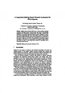
2. Related Works FPGA accelerators for FDTD computation with simple boundary conditions are already implemented in previous works [5–7]. Although those works use different design methods such as OpenCL [16], HDL, or MaxCompiler [18], the basic architecture is very similar. To explain the accelerator architecture, we consider a simple example of 2D stencil computation as shown in Figure 1. Note that FDTD method is also regarded as a stencil computation. Figure 1(a) shows the data streaming order in a 2D 𝑛𝑥 × 𝑛𝑦 grid. A grid-point is called a cell. Data of the cells are streamed from left-to-right along the 𝑖 axis and bottom-to-top along the 𝑗 axis. Figure 1(b) shows the computations of two consecutive iterations. To compute cell(1, 1) in the iteration 𝑡 + 1 (Cell𝑡+1 (1, 1)), data of its surrounding cells belonging to the iteration 𝑡 are required. When the computation of cell(2, 2) is in progress in the iteration 𝑡 (Cell𝑡 (2, 2)), all the data required for the computation of cell(1, 1) are available. Therefore, the computations of cell(2, 2) in iteration 𝑡 and cell(1, 1) in iteration 𝑡 + 1 can be done in parallel. We call this “iteration-parallel” computation. Detailed description of the iteration-parallel computation can be found in [19]. Figure 2 shows the flowchart of the whole computation. Computations of 𝑑 iterations are done in parallel on FPGA. If the total number of iterations is larger than 𝑑 (which is the usual case), the FPGA computation is done for “𝑡𝑜𝑡𝑎𝑙_𝑖𝑡𝑒𝑟𝑎𝑡𝑖𝑜𝑛𝑠/𝑑” times. In this method, the global memory is read once in each 𝑑 iteration. Iteration-parallel computation reduces the global memory access while allowing sufficient amount of parallel operations.

International Journal of Reconfigurable Computing The works in [5–7] propose FPGA accelerators based on iteration-parallel computation. A high level design tool called MaxCompiler [18] is used in [5] to accelerate 3D FDTD computation. OpenCL is used in [6, 7] for 2D FDTD computation. Although these works use iteration-parallelism to increase the processing speed, they only support simple boundary conditions such as fixed boundaries where constants are used as the boundary data. The works in [8–10] propose FPGA accelerators that support complex boundary conditions. Impedance boundary condition is used in [8]. In terms of computation, impedance boundary is more complex compared to a fixed boundary, since it requires more computations. In terms of data dependency, it is easy to implement since the outputs are produced in the same order of the input data stream. However, it can be used only for 2D FDTD and the computations are done in 32-bit fixed point. Therefore, the usage of such an accelerator is severely restricted. Absorbing boundary conditions are supported by the FPGA accelerator proposed in [9]. However, it has not considered the periodic boundary conditions. The work in [10] is one the very few works that proposes an FPGA accelerator to compute both absorbing and periodic boundary conditions. The boundary-related data streamed out from the FPGA to the CPU through the PCI express bus. They are processed in the CPU and streamed into the FPGA after the computation of the core area is finished. In this method, the frequent data transfers and synchronizations between CPU and FPGA reduce the performance. Although the accelerators in [8–10] process boundary conditions, they have not used the iteration-parallel computation which is the most efficient way on FPGAs to increase the processing speed. Since the boundary conditions distort the regularity of the data flow, it is usually difficult to implement the iterationparallelism.

3. FPGA Accelerator for 3D FDTD Computation 3.1. 3D FDTD with Periodic Boundary Conditions. In this section, we explain the FPGA acceleration for 3D FDTD computation when there are periodic and absorbing boundary conditions. Figure 3 shows the simulation area. Simulating very large grids could take enormous amount of processing time. Instead, we divide the grid into multiple boxes and consider that the same unit-box is replicated. We use periodic boundary conditions to correctly update the box. Using this method, we can reduce the computation amount significantly. This method is used for real-world FDTD simulations in many works such as [20–22]. Figure 4 shows the 3D computation domain of the unitbox. It contains six boundaries and the core. A cell in this 3D domain is denoted by the coordinates 𝑖, 𝑗, and 𝑘. The electric fields 𝐸𝑥 , 𝐸𝑦 , and 𝐸𝑧 belonging to three directions are computed in each cell. The computations are classified into the core area and the boundary area computations. Absorbing boundary conditions are used to compute the top and the bottom boundaries (𝑖𝑗 boundaries), while periodic boundary conditions are used for the other four boundaries (𝑖𝑘 and

International Journal of Reconfigurable Computing

3

ny

j j

Order of the data flow

ny j

Cellt(2, 2)

···

···

2

2

1

1

0

0 0

(0, 0)

Cellt+1 (1, 1)

i

1

2

· · · nx − 1 i

Iteration t

0

1

2

· · · nx − 1 i

Iteration t+1

(b) Parallel computation of the cells in multiple iterations. Computations of Cell𝑇 (2, 2) and Cell𝑇+1 (1, 1) can be done in parallel

(a) Order of the data flow

Figure 1: 2D stencil computation using 𝑛𝑥 × 𝑛𝑦 grid. Iterations 𝑡 and 𝑡 + 1 are computed in parallel.

Host CPU

FPGA

Data transfer (host → FPGA)

External memory

Kernel execution

Computation of d iterations in parallel

Unit-box ⋱

···

External memory

Kernel execution .. .

Computation of d iterations in parallel

z

External memory

y x

Figure 3: Simulation area and unit-box. Kernel execution

Computation of d iterations in parallel

Data transfer (FPGA → host)

External memory ij boundary k = nz − 1

ik boundary j = ny − 1

Figure 2: Flowchart of the computation. FPGA processes 𝑑 iterations in parallel.

𝑗𝑘 boundaries). Figure 5 shows a cross section of the computation domain that represents one 𝑖𝑗 plane. To compute the electric fields of cell(0, 𝑗, 𝑘), we need the data of the cell(𝑛𝑥 − 2, 𝑗, 𝑘) of the same iteration. Therefore, the cell(𝑛𝑥 − 2, 𝑗, 𝑘) must be computed before computing the cell(0, 𝑗, 𝑘). This is against the order of the input data stream shown in Figure 1(a). Figure 6 shows the flowchart of the 3D FDTD algorithm. In usual Yee’s FDTD algorithm [1], both the first-order differential equations of electric and magnetic fields are calculated. However, if we are interested only in electric field, we can simply substitute the magnetic field terms by equations that only contain electric field terms. The details of this method

jk boundary i=0

Core

jk boundary i = nx − 1

ik boundary j=0 k j

i

ij boundary k=0

Periodic boundary conditions: ik, jk boundaries Absorbing boundary conditions: ij boundaries

Figure 4: 3D computation domain of a unit-box.

4

International Journal of Reconfigurable Computing and also some constants such as 𝑅1 ∼𝑅4 and ssn. Note that the computations of 𝐸𝑦 and 𝐸𝑧 are also done similar to

Et+1 (0, y, z) = f(Et+1 (nx − 2, y, z)) Et+1 (nx − 1, y, z) = f(Et+1 (1, y, z))

Cell(nx − 1, ny − 1, z)

1 1 𝑘) + ssn (𝑖 + , 𝑗, 𝑘) × {𝑅1 × {𝐸𝑥𝑡 (𝑖 + , 𝑗 + 1, 𝑘) 2 2

ij plane k

1 1 − 2𝐸𝑥𝑡 (𝑖 + , 𝑗, 𝑘) + 𝐸𝑥𝑡 (𝑖 + , 𝑗 − 1, 𝑘)} + 𝑅2 2 2

j Cell(0, 0, z) i

Cell(nx − 1, 0, z)

Figure 5: Data dependency on the boundaries.

No

If (t < ttotal )

Electric field computation Et+1 (core) = func(Et , Et−1 )

Periodic boundary conditions Et+1 (PBC) = func(Et+1 (core))

Absorbing boundary conditions E

1 1 × {𝐸𝑥𝑡 (𝑖 + , 𝑗, 𝑘 + 1) − 2𝐸𝑥𝑡 (𝑖 + , 𝑗, 𝑘) 2 2 1 1 + 𝐸𝑥𝑡 (𝑖 + , 𝑗, 𝑘 − 1)} − 𝑅3 × {𝐸𝑦𝑡 (𝑖 + 1, 𝑗 + , 𝑘) (1) 2 2 1 1 − 𝐸𝑦𝑡 (𝑖 + 1, 𝑗 − , 𝑘) + 𝐸𝑦𝑡 (𝑖, 𝑗 − , 𝑘) 2 2 1 1 − 𝐸𝑦𝑡 (𝑖 + , 𝑗, 𝑘)} − 𝑅4 × {𝐸𝑧𝑡 (𝑖 + 1, 𝑗, 𝑘 + ) 2 2

Yes

t+1

1 1 1 𝐸𝑥𝑡+1 (𝑖 + , 𝑗, 𝑘) = 2𝐸𝑥𝑡 (𝑖 + , 𝑗, 𝑘) − 𝐸𝑥𝑡−1 (𝑖 + , 𝑗, 2 2 2

t

t+1

(ABC) = func(E , E

1 1 − 𝐸𝑧𝑡 (𝑖 + 1, 𝑗, 𝑘 − ) + 𝐸𝑧𝑡 (𝑖, 𝑗, 𝑘 − ) 2 2 1 − 𝐸𝑧𝑡 (𝑖, 𝑗, 𝑘 + )}} . 2 Constant data set ssn contains wave impedance and refractive index data. It is given by 𝑠 = CFL × 𝑠min ,

(core))

ssn (𝑖, 𝑗, 𝑘) = t= t+1

Figure 6: Flowchart of the 3D FDTD algorithm.

are available in [23, chapter 2]. Since the same equations are used, the physical model and the numerical values are the same as Yee’s algorithm. However, we need the electric field data of the current and the previous iteration to compute the next iteration. In each iteration, both periodic and absorbing boundary data are computed. The periodic boundary data of iteration 𝑡 + 1 are computed using the electric field data of the same iteration. The absorbing boundary data are computed using the electric field data of the iterations 𝑡 and 𝑡 + 1. Since the boundary computations require the data of the core cells, data dependencies exist among different cells of the same iteration. Therefore, the computations of the current iteration must be completed before starting the computations of the next iteration. Due to this problem, we cannot use the existing methods that are based on the iteration-parallel computation. The computation of the electric field in 𝑥 direction at time step 𝑡 + 1 (𝐸𝑥𝑡+1 ) is shown in (1). To compute 𝐸𝑥𝑡+1 , we need the electric field data at the time steps 𝑡 and 𝑡 − 1. We also need the electric field data in 𝑦 and 𝑧 directions at the time step 𝑡

2 𝑠min

2

𝑟 (𝑖, 𝑗, 𝑘)

.

(2)

Note that 𝑟(𝑖, 𝑗, 𝑘) is the refractive index data for each coordinate, and it is given initially as an input data file. The minimum value of the refractive index data is given by 𝑠min . The stability constant is given by CFL and we use the value 0.99. The values of 𝑠 and ssn(𝑖, 𝑗, 𝑘) do not change with iterations. Those are constants for all iterations. Therefore, we can compute those on CPU and the processing time required for this computation is very small, compared to the processing time of the whole FDTD computation. 3.2. Data Flow Regulation. Our goal in the proposed implementation is to maintain the regularity of the input and output data streams even when there are boundary conditions. However, as explained in Section 3.1, the order of the computations is different from that of the input data stream. To solve this problem, we regulate the output data stream by reordering the computed data. For example, let us consider the 𝑖𝑗-plane shown in Figure 5 and assume that 𝑛𝑥 = 8 and 𝑘 = 𝑚. We consider the computations of the cells(0, 1, 𝑚) to (7, 1, 𝑚) when 𝑗 = 1 on 𝑖𝑗-plane. In this example, the data of the core cell(6, 1, 𝑚) are required to compute the boundary cell(0, 1, 𝑚). Let us assume that the data of cell(6, 1, 𝑚) is computed at the clock cycle 𝑇. Using the data of the cell(6, 1, 𝑚) as the input, we can compute the boundary cell(0, 1, 𝑚) at the clock cycle 𝑇 + 1. To maintain the regularity of the output

International Journal of Reconfigurable Computing

5

··· ··· Et−1 (2)

Regulate data order

Et−1 (nx − 3)

Computation (boundary data)

Et−1 (nx − 2)

Computation (core data)

Et−1 (nx − 1)

Et (nx − 1)

Etemp (nx − 2)

Et (nx − 2)

Etemp (nx − 3) ···

E

temp

E

Et−1 (0)

Computation and data stream regulation

Et (nx − 3) ···

Etemp (2) temp

Et−1 (1)

Input data stream

Etemp (nx − 1)

(1) (0)

··· Et (1) Et (0)

Output data stream (next PCM)

Figure 7: Proposed pipelined computation module (PCM). Computed data are arranged in the correct order to preserve the regularity of the data flow.

data stream, the output data should be in the order of cells(0, 1, 𝑚), (1, 1, 𝑚), (2, 1, 𝑚), . . . , (6, 1, 𝑚). If the data of the cell(0, 1, 𝑚) is released to the output data stream at the clock cycle 𝑇 + 1, the data of the cell(6, 1, 𝑚) must be released at the clock cycle 𝑇 + 7 and even it was computed before the cell(0, 1, 𝑚). That is, the data of the cell(6, 1, 𝑚) must be stored for 7 clock cycles before being released to the output data stream. Similarly, the core data of the cells(1, 1, 𝑚), . . . , (5, 1, 𝑚) also have to be delayed for 7 cycles each. Figure 7 shows the proposed pipelined computation module (PCM) of our FPGA accelerator. It contains modules to compute core and the boundary data and a shift-register array to store the computed data. The input data streamed into the PCM in a regular pattern. The computation of the core starts before the boundaries. The computed data are written to the appropriate locations of the shift-register array. The locations of the shift-register array are calculated in such a way to preserve the data order. According to the example in Figure 5, the data of the cell(6, 1, 𝑚) is stored in seven places after the data of the cell(0, 1, 𝑚), irrespective of the order of the computation. After the data area is arranged in the correct order, they are released to the output stream. Figure 8 shows the overall architecture. It consists of 𝑑 PCMs where each of which processes one iteration. This architecture is very similar to the one discussed in [5–7]. The difference is the structure of a PCM which can process both core and boundary data and also produces a regular output data stream. To compute the electric field of the next iteration, we need the data of the current and the previous iterations. Fortunately, they are already available in the shift-registers of the current and the previous PCMs. For example, if we have 3 PCMs, the initial data of the iteration 𝑡 − 1 and the data of three iterations 𝑡, 𝑡 + 1 and 𝑡 + 2 are available simultaneously. Therefore, 𝑑 PCMs and an additional shift-register array are

sufficient to compute 𝑑 iterations in parallel as shown in Figure 8. However, there are a few disadvantages in this method. Since we have to use shift-registers to temporally store the computed data, the area of a PCM is increased. As a result, the number of PCMs can be decreased so that the processing time can be increased. The computed data have to be stored for several clock cycles until they are arranged correctly. This increases the latency and also the processing time. 3.3. OpenCL-Based Implementation and Optimization. This section explained how to implement and optimize the proposed FPGA accelerator using OpenCL [16]. OpenCL is a framework to write programs to execute across a heterogeneous parallel platform that consists of a host and devices. “Intel FPGA SDK for OpenCL” [24] is used for FPGA and CPU based systems, where the CPU is the host and the FPGA is the device. The “kernels” are the functions executed on FPGA and they are implemented using OpenCL. The inputs for the kernels are transferred from the host, and the outputs are transferred back to the host. Listing 1 shows an extract of a C-program used to compute the electric field in 𝑥 direction according to (1). Arrays 𝐸𝑓𝑥, 𝐸𝑛𝑥, and 𝐸𝑝𝑥 are used to store the data of the electric fields in iterations 𝑡 + 1, 𝑡, and 𝑡 − 1, respectively. The electric fields at the coordinates 𝐸𝑥𝑡 (𝑖 + 1/2, 𝑗, 𝑘) and 𝐸𝑥𝑡 (𝑖 − 1/2, 𝑗, 𝑘) are represented by array indexes Enx[i][j][k] and Enx[i−1][j][k], respectively. Similar method is used to compute electric fields in 𝑦 and 𝑧 directions. Note that (𝑖, 𝑗, 𝑘) notation is used for the cell coordinates in equations, and [i][j][k] notation is used to show the data array indexes used in the C-program. Since 𝐸𝑥 is defined at cell(𝑖 + 1/2, 𝑗, 𝑘) as shown in (1), we have to use the average of ssn[i+1][j][k] and

6

International Journal of Reconfigurable Computing

FPGA board

Host computer

PCM 1

PCM 2

···

···

Computation and data order regulation

Computation and data order regulation

Computation and data order regulation

Shift registers

DRAM

PCM d

Figure 8: Architecture of the proposed FPGA accelerator. Iteration-parallel computation is achieved by processing 𝑑 iterations in parallel.

ssn[i][j][k] to determine ssn at 𝑥 direction (ssnx). Similar process is applied to compute ssny and ssnz also, as shown in Listing 2. Note that arrays ssnx, ssny, and ssnz are used in the C-program to store the data of ssn𝑥 , ssn𝑦 , and ssn𝑧 , respectively. Constants ssn𝑥 , ssn𝑦 , and ssn𝑧 are the ssn values of 𝑥, 𝑦, and 𝑧 directions, respectively. To calculate the electric fields 𝐸𝑥 , 𝐸𝑦 , and 𝐸𝑧 of a cell, we have to load nine data values that include electric field data of the present and the previous iterations of all three directions (Enx,Epx,Eny,Epy,Enz,Epz) and constants (ssnx,ssny,ssnz). If all the data are stored in different off-sets in the global memory, we require at least 9 “load transactions.” To reduce the amount of transactions, we use an array-of-structure in the global memory to store the data. Each element in the array has the data of the present and the previous electric fields and the constants. Therefore, one array element provides all the data necessary to compute one cell. One array element contains 36 bytes (9 × 𝑠𝑖𝑧𝑒 𝑜𝑓 (float)) in single precision and 72 bytes in double precision. On the other hand, one memory load/store transaction accesses 64 bytes from the global memory. If the data are not aligned, one or two transactions are required to access an array element. If the data are aligned to 64-byte boundary, only one transaction is required. Similarly, two memory transactions are required to load one array element in double precision for aligned data and more than two are required for nonaligned data. To reduce the amount of memory transactions, we have to reduce the data amount of one array element. To reduce the data amount, we compute the constant in the FPGA instead of loading the already computed ones from the memory. For example, if we compute ssnx and ssny on FPGA, we have to load only ssn and ssnz from the memory. This reduces 4 bytes per cell. If we reduce the size of an array element to 32 bytes, we can load two array elements in one transaction. The computations of the constants can be done in parallel to

the computations of the electric fields. However, it requires additional computation units and increases the logic area of the FPGA. Algorithm 1 shows the pseudo code of the computation kernel of the accelerator. The inputs and outputs of the kernel are represented by the array-of-structures in line (1). After an array element is read, the current and the previous electric field data of all three directions and constants are stored in the shift-registers. Shift-registers are included in each PCM to store the data of its inputs from the previous PCM. Shiftregisters are defined using two-dimensional arrays as shown from line (2) in Algorithm 1. One array dimension represents the number of PCMs and the other represents the lifetime of the data. The lifetime represents the number of steps that one data value should be stored in the FPGA until it is no longer required for any further computation. Note that the lifetime is quite large since the output of one iteration is used in next two iterations. We also need another set of shift-registers to temporally store the computed data in order to regulate the data order. Those shift-registers are shown from line (5). The lifetime of the data stored in those shift-registers is small since the data are used in the same iteration. The behaviors of the shift-registers are coded from lines (8) to (29). The computations of the cells in the core and the boundary are shown from line (37). Note that the computed data are temporary stored in the shift-registers to regulate the output data stream. The locations the shift-registers are determined by processing some conditional branches as shown from line 37. After the output data are available and the order is fixed, data are written to the shift-registers of the next PCM. If it is the last PCM, data are written back to the global memory.

4. Evaluation For the evaluation, we use two FPGA boards, two GPUs, and two multicore CPUs. The FPGA boards are DE5 [25] and

International Journal of Reconfigurable Computing

(1) _kernel FDTD (global struct ∗ 𝑑𝑖𝑛, global struct ∗ 𝑑𝑜𝑢𝑡) (2) 𝐸𝑥 [𝑑 + 1][𝑙𝑖𝑓𝑒𝑡𝑖𝑚𝑒] (3) 𝐸𝑦 [𝑑 + 1][𝑙𝑖𝑓𝑒𝑡𝑖𝑚𝑒] (4) ⋅⋅⋅ (5) 𝐸𝑥𝑡𝑚𝑝 [𝑑][𝑡𝑚𝑝𝑡𝑖𝑚𝑒] (6) ⋅⋅⋅ (7) while 𝑐𝑜𝑢𝑛𝑡 ≠ 𝐿𝑜𝑜𝑝 𝑖𝑡𝑒𝑟𝑎𝑡𝑖𝑜𝑛𝑠 do (8) #pragma unroll (9) for 𝑖 = (𝑙𝑖𝑓𝑒𝑡𝑖𝑚𝑒 − 1) → 𝑖 = 1 do (10) #pragma unroll (11) for 𝑗 = 0 → 𝑗 = 𝑑 do (12) 𝐸𝑥 [𝑗][𝑖] = 𝐸𝑥 [𝑗][𝑖 − 1] (13) 𝐸𝑦 [𝑗][𝑖] = 𝐸𝑦 [𝑗][𝑖 − 1] (14) ⋅⋅⋅; (15) end (16) end (17) #pragma unroll (18) for 𝑖 = (𝑡𝑚𝑝𝑡𝑖𝑚𝑒 − 1) → 𝑖 = 1 do (19) #pragma unroll (20) for 𝑗 = 0 → 𝑗 = 𝑑 − 1 do (21) 𝐸𝑥𝑡𝑚𝑝 [𝑗][𝑖] = 𝐸𝑥𝑡𝑚𝑝 [𝑗][𝑖 − 1] (22) 𝐸𝑦𝑡𝑚𝑝 [𝑗][𝑖] = 𝐸𝑦𝑡𝑚𝑝 [𝑗][𝑖 − 1] (23) ⋅⋅⋅; (24) end (25) end (26) 𝐸𝑥 [0][0] = 𝑑𝑖𝑛[𝑐𝑜𝑢𝑛𝑡] ⋅ 𝐸𝑥𝑝𝑟𝑒V ; (27) ⋅⋅⋅; (28) 𝐸𝑥 [1][0] = 𝑑𝑖𝑛[𝑐𝑜𝑢𝑛𝑡] ⋅ 𝐸𝑥𝑐𝑢𝑟𝑟 ; (29) ⋅⋅⋅; (30) #pragma unroll (31) for 𝑗 = 0 → 𝑗 = (𝑑 − 1) do (32) //compute the temporary storage locations (33) 𝑐𝑜𝑛𝑑𝑖𝑡𝑖𝑜𝑛 1: (𝑎𝑑𝑟𝑎 , . . . , 𝑎𝑑𝑟𝑝 , . . .) (34) 𝑐𝑜𝑛𝑑𝑖𝑡𝑖𝑜𝑛 2: (𝑎𝑑𝑟𝑎 , . . . , 𝑎𝑑𝑟𝑝 , . . .) (35) ⋅⋅⋅ (36) //Computation of the core data (37) 𝐸𝑥𝑡𝑚𝑝 [𝑗][𝑎𝑑𝑟𝑎 ] = 𝑓𝑢𝑛𝑐(𝐸𝑥 [𝑗][⋅], 𝐸𝑥 [𝑗 + 1][⋅]) (38) ⋅⋅⋅ (39) //Computation of the boundary data (40) 𝐸𝑥𝑡𝑚𝑝 [𝑗][𝑎𝑑𝑟𝑝 ] = 𝑓𝑢𝑛𝑐(𝐸𝑥𝑡𝑚𝑝 [𝑗][⋅]) (41) ⋅⋅⋅ (42) if 𝑐𝑜𝑢𝑛𝑡 > 𝑗 × 𝑙𝑎𝑡𝑒𝑛𝑐𝑦 then (43) if 𝑗 == 𝑑 then (44) 𝑑𝑜𝑢𝑡[𝑎𝑑𝑟𝑠] ⋅ 𝐸𝑥𝑝𝑟𝑒V = 𝐸𝑥 [𝑗][⋅]; (45) ⋅⋅⋅; (46) 𝑑𝑜𝑢𝑡[𝑎𝑑𝑟𝑠] ⋅ 𝐸𝑥𝑐𝑢𝑟𝑟 = 𝐸𝑥𝑡𝑚𝑝 [𝑗][⋅]; (47) ⋅⋅⋅ (48) else (49) 𝐸𝑥 [𝑗 + 2][0] = 𝐸𝑥𝑡𝑚𝑝 [𝑗][⋅]; (50) ⋅⋅⋅ (51) end (52) end (53) end (54) 𝑐𝑜𝑢𝑛𝑡 + +; (55) end (56) end Algorithm 1: Pseudo code of the stencil computation kernel.

7

8

International Journal of Reconfigurable Computing

E2 = Enx[i][j][k]+Enx[i][j][k]; Efx[i][j][k]= E2−Epx[i][j][k]+ssnx[i][j][k]⋆ ( R[0]⋆(Enx[i][j+1][k]−E2+Enx[i][j−1][k]) +R[1]⋆(Enx[i][j][k+1]−E2+Enx[i][j][k−1]) −R[2]⋆(Eny[i+1][j][k]−Eny[i+1][j−1][k]+ Eny[i][j−1][k]−Eny[i][j][k]) −R[3]⋆(Enz[i+1][j][k]−Enz[i+1][j][k−1]+ Enz[i][j][k−1]−Enz[i][j][k])); Listing 1: Extract of a C-program that shows the computation of 𝐸𝑥 .

ssnx[i][j][k]=(ssn[i][j][k]+ssn[i+1][j][k])/2 ssny[i][j][k]=(ssn[i][j][k]+ssn[i][j+1][k])/2 ssnz[i][j][k]=(ssn[i][j][k]+ssn[i][j][k+1])/2 Listing 2: Computation of constants.

395-D8 [26]. FPGAs are configured using Quartus 16.0 with SDK for OpenCL. The CPU code is written in C language with OpenMP directives and compiled using Intel C compiler 2016 (Intel Parallel Studio XE 2016) with relevant optimization options. GPU code is written in CUDA C code considering multithreaded data-parallel computation. GPUs are programmed using CUDA 7.5 compiler. The operating system is CentOS 6.7. We use a unit-box that has a periodic structure for the simulation. It is 960 nm × 960 nm × 9,540 nm long in 𝑥, 𝑦, and 𝑧 dimensions, respectively. The objective of the simulation is to find various optical phenomena such as guided-mode resonance, at the wavelength range of 1,000 nm∼2,000 nm. To simulate such resonance phenomena, a fine spatial mesh is needed. Thus, we set the grid division as 20 nm for each direction. This leads to a grid of 48 × 48 × 477 in each 𝑖, 𝑗, and 𝑘 axis, respectively. Note that the grid size is given by parameters in the OpenCL code, and we can use a different grid by changing the values of the parameters. Computation is done for 8,192 iterations. Table 1 shows the comparisons of the accelerators with different data access methods. We used DE5 board that contains Stratix V 5SGXEA7N2F45C2 FPGA. The computations are done in single-precision floating point. Method (1) uses “noncoalesced” memory access since it loads 9 data values from different locations in the global memory. Therefore, nine memory transactions are required for the computation of a cell. Since one transaction loads 64 bytes of data, the computations of the neighboring cells can be done by accessing the cache instead of the global memory. Memory access is coalesced in method (2) by using an array-of-structures. An array element contains 36 bytes so that the data are not aligned to the 64-byte boundary of a transaction. As a result, multiple transactions are required to access array elements, and the processing time is increased compared to method (1). This problem is easily solved in method (3) by aligning the data to the 64-byte boundary. After the data are aligned, only a single transaction is required to access an array element.

Moreover, the clock frequency is also improved due to the simplicity of the data access. As shown in Table 1, the processing time is reduced significantly compared to method (2). In method (4), the memory access is further reduced by decreasing the input data amount. It is done by computing the constants ssnx and ssny inside the FPGA in every cycle, instead of loading precalculated constants from the memory. Using this method, we reduce the size of an array element to 32 bytes so that two array elements can be read in a single transaction. The clock frequency is improved and the processing time is reduced significantly compared to method (3). In method (5), the size of an array element is further reduced to 28 bytes by computing all constants (ssnx,ssny,ssnz) on FPGA. However, this has increased the number of access points to ssn as shown in Listing 2. Moreover, the logic area is increased compared to method (4). Some of these reasons could be the cause for the processing time increase and clock frequency reduction. The best balance of the computation and the memory access is achieved in method (4) and it is the fastest implementation. Table 2 shows the comparisons against the CPU and GPU based implementations. In this comparison, we used singleprecision floating-point computation. The processing speed using DE5 FPGA board is 3.3 times and 1.5 times higher compared to those of the CPUs and GPUs, respectively. The processing speed using 395-D8 FPGA board is also higher than those of the CPUs and GPUs. The performances of GPUs are very sensitive to the memory bandwidth. Recent high-end GPU such as K40 with 288 GB/s bandwidth could provide better performance compared to this work. However, we believe that our evaluation using GTX680 (192.2 GB/s bandwidth) is a reasonable one, since it has a similar bandwidth compared to the high-end K20 GPU. In addition, it would be fair to compare devices such as Stratix V and GTX680, which are available in the same era. Despite having lower bandwidth and peak performance, DE5 FPGA gives the highest processing speed. Note that the peak performance of the FPGAs is calculated according to [27]. Unlike CPUs and GPUs, FPGAs are reconfigurable devices, and we can design the most suitable architecture for a given application considering its operations. We can use the resources efficiently by designing computing units that do only the required computation. The comparison using double-precision floating-point computations is shown in Table 3. Although FPGAs give better performance compared to CPUs, they cannot beat the performances of the GPUs. Double-precision performance on FPGA is around 25% of the single-precision performance. The current generation FPGAs (Stratix V series) do not have dedicated floating-point units. Multiplications are done in DSPs and the additions are done using logic blocks. Due to the large logic block requirement for double-precision computation, the performances are decreased. However, the nextgeneration FPGAs such as Aria 10 and Stratix 10 devices contain dedicated floating-point units. Therefore, we can expect a significant reduction of the logic area and increase of the processing speed.

International Journal of Reconfigurable Computing

9

Table 1: Comparison of the FPGA accelerators with different data access methods using DE5 board. Method

Processing time (s)

ALMs

Registers

8.01 14.75 9.42 6.31 6.69

179,925 (77) 176,370 (75) 170,692 (73) 175,032 (75) 176,637 (75)

368,483 (39) 357,220 (38) 349,960 (37) 357,283 (38) 359,472 (38)

(1) Noncoalesced (36 bytes/cell) (2) Coalesced (36 bytes/cell, nonaligned) (3) Coalesced (36 bytes/cell, aligned) (4) Coalesced (32 bytes/cell, aligned) (5) Coalesced (28 bytes/cell, aligned)

Area (%) Memory (kByte) 2,911 (45) 3,012 (47) 2,958 (45) 2,595 (41) 2,363 (36)

DSPs

RAM blocks

114 (45) 114 (45) 114 (45) 114 (45) 114 (45)

2,050 (80) 1,953 (76) 1,879 (73) 1,750 (68) 1,618 (63)

Frequency (MHz) 205.6 206.7 217.8 260.0 243.6

Table 2: Comparison with GPUs and CPUs using single-precision floating-point computation. FPGA Number of cores1 Core clock frequency (MHz) Memory bandwidth (GB/s) Peak performance (Gflop/s) Processing time (s) 1

DE5 — 260 25.6 193 6.31

GPU 395-D8 — 193 34.1 1502.9 7.36

GTX680 1152 980 192.2 3090 9.39

GTX750Ti 1024 1127 86.4 1305 10.71

Multicore CPU i7-4960x E5-1650 v3 6 6 3600 3500 51.2 59.7 345.6 672 23.63 20.84

GPU: CUDA cores; multicore CPU: CPU cores.

Table 4 shows the comparisons with other recent works that propose FPGA accelerators for 3D FDTD. All computations are done in single-precision floating point. The accelerator proposed in [9] provides 1000 mega cell/s processing speed using absorbing boundary conditions. However, it has not used periodic boundary conditions. Accelerators proposed in [5, 10] provide 325 and 1,820 mega cell/s processing speeds, respectively, for fixed boundary conditions. When absorbing boundaries are used, the performance of [10] is reduced to 65.5%. When periodic boundary conditions are used, the performance is reduced to just 5.5% and 8.4%, respectively, comparing with the ones that use fixed and absorbing boundary conditions. The accelerator proposed in this paper provides 1,427 mega cells/s processing speed on a single FPGA even using both absorbing and periodic boundary conditions together. This is a 14.2 times improvement compared to [10]. Since we used a single FPGA compared to four FPGAs in [10], our achievement is significant. Memory bandwidths of the method in [10] are 26.8 GB/s and 29.9 GB/s when using fixed and absorbing boundaries, respectively. MAX3 board with Virtex-6 FPGAs used in [10] has a theoretical memory bandwidth of 38.6 GB/s, so that the accelerator is not memory bound. The theoretical memory bandwidth of the DE5 board used in this work is 25.6 GB/s. If the method in [10] is implemented on the DE5 board, it will become memory bound and would perform worse compared to the implementation on MAX3. On the other hand, our method uses only 13.4 GB/s bandwidth so that it is not memory bound in either of the FPGA boards. We use a single but very deep pipeline so that the application does not become memory bound. However, [10] uses multiple but shorter pipelines in parallel, and that requires reasonably large bandwidth. When [10] uses both absorbing and periodic boundaries, the boundary data are processed in the host CPU. This

requires frequent data transfers between host and FPGA. Such transfers depend on the PCIe bandwidth, and it is much lower than the memory bandwidth. Moreover, there could be some control overheads, synchronizing overheads, and so on that slow down the computation. Table 5 shows the performance comparison against FPGA accelerators that use simple boundary conditions. All the implementations are done on DE5 FPGA board using singleprecision floating-point computation. The 2D FDTD computation with fixed boundaries can be regarded as one of the simplest FDTD computations. The most recent and the fastest implementation of the 2D FDTD computation is proposed in [7]. It produces 150.3 Gflop/s of processing speed. We also measured the performance of the 3D FDTD computation with absorbing boundaries. It produces 98.5 Gflop/s of processing speed. The proposed 3D FDTD computation with absorbing and periodic boundary conditions produces 89.9 Gflop/s of processing speed. The performance of the proposed method is slightly small compared to the 3D FDTD implementation with only absorbing boundaries. However, the performance is reduced to nearly 60% compared to the 2D FDTD with fixed boundaries. Despite this reduction, we believe that retaining nearly 60% of the processing speed of the simplest 2D FDTD and yet processing the complex boundary conditions is a significant achievement. We may improve the performance using manual HDLbased designs. However, we believe that the gap between the performances of OpenCL-based and HDL-based designs is getting narrower. In our earlier work in [7], we found that OpenCL-based design provides 76% of the FPGA peak performance for 2D FDTD with fixed boundaries. In this paper, we achieved over 51% of the peak performance for 3D FDTD with absorbing boundary and 46% of the peak performance with both absorbing and periodic boundaries. Moreover, the

10

International Journal of Reconfigurable Computing Table 3: Comparison with GPUs and CPUs using double-precision floating-point computation. FPGA

Core clock frequency (MHz) Processing time (s)

DE5 252 28.09

GPU 395-D8 209 25.24

GTX680 980 14.44

Multicore CPU i7-4960x E5-1650 v3 3600 3500 69.45 62.13

GTX750Ti 1127 20.61

Table 4: Comparison with other FPGA accelerators for 3D FDTD with boundary conditions. Method

Boundary conditions

FPGA

Work in [9]

ABC

Work in [5]

fixed

n/a Xilinx Virtex-6 XC6VSX475T

fixed Work in [10]

Clock frequency MHz

Achieved throughput (maximum bandwidth) GB/s

1,000

50

n/a

325

100

n/a

1,820 Xilinx Virtex-6 XC6VSX475T × 4

fixed and ABC ABC and PBC

This paper

Performance mega cell/s

1,193

26.8 (38.6) 100

100 Altera Stratix-V 5SGXEA7N2F45C2

ABC and PBC

1,427

29.9 (38.6) n/a

260

13.4 (25.6)

n/a: not available.

Table 5: Performance comparison against FPGA accelerators that use simple boundary conditions. Method

Boundary conditions

2D FDTD [6] fixed 3D FDTD ABC 3D FDTD (this ABC and PBC paper)

Performance (Gflop/s)

Frequency (MHz)

150.3 98.5

291 261

89.9

260

work in [28] reports that, although HDL-based designs use less resources compared to OpenCL-based designs, there is not much difference in the clock frequency and performance.

5. Conclusion We have proposed an FPGA accelerator for 3D FDTD that efficiently supports absorbing and periodic boundary conditions. The data flow is regulated in a PCM after the computation of the boundary data. This allows data streaming between multiple PCMs, so that we can implement iterationparallel computation. The FPGA architecture is implemented using OpenCL. Therefore, we can use it for different applications and boundary conditions by just changing the software code. Since OpenCL is a system design method, we can implement the proposed accelerator on any system that contains an OpenCL-capable FPGA. According to the experimental results, we achieved over 3.3 times and 1.5 times higher processing speeds compared to the CPUs and GPUs, respectively. Moreover, the proposed accelerator is more than 14 times faster compared to the recently proposed FPGA

accelerators that are capable of handling boundary conditions.

Conflicts of Interest The authors declare that there are no conflicts of interest regarding the publication of this paper.

References [1] K. S. Yee, “Numerical solution of initial boundary value problems involving Maxwell’s equations in isotropic media,” IEEE Transactions on Antennas and Propagation, vol. 14, no. 3, pp. 302–307, 1966. [2] F. Zepparelli, P. Mezzanotte, F. Alimenti et al., “Rigorous analysis of 3D optical and optoelectronic devices by the Compact-2DFDTD method,” Optical and Quantum Electronics, vol. 31, no. 9, pp. 827–841, 1999. [3] M. A. Jensen and Y. Rahmat-Samii, “Performance analysis of antennas for hand-held transceivers using FDTD,” IEEE Transactions on Antennas and Propagation, vol. 42, no. 8, pp. 1106– 1113, 1994. [4] Y. Takei, H. M. Waidyasooriya, M. Hariyama, and M. Kameyama, “FPGA-oriented design of an FDTD accelerator based on overlapped tiling,” in Proceedings of the International Conference on Parallel and Distributed Processing Techniques and Applications (PDPTA ’15), pp. 72–77, Las Vegas, Nev, USA, 2015. [5] K. Okina, R. Soejima, K. Fukumoto, Y. Shibata, and K. Oguri, “Power performance profiling of 3-D stencil computation on an FPGA accelerator for efficient pipeline optimization,” ACM SIGARCH Computer Architecture News, vol. 43, no. 4, pp. 9–14, 2016. [6] H. M. Waidyasooriya and M. Hariyama, “FPGA-based deeppipelined architecture for FDTD acceleration using OpenCL,” in Proceedings of the IEEE/ACIS 15th International Conference

International Journal of Reconfigurable Computing

[7]

[8]

[9]

[10]

[11]

[12]

[13]

[14]

[15]

[16] [17]

[18] [19]

[20]

[21]

[22]

on Computer and Information Science (ICIS ’16), pp. 109–114, Okayama, Japan, June 2016. H. M. Waidyasooriya, Y. Takei, S. Tatsumi, and M. Hariyama, “OpenCL-based FPGA-platform for stencil computation and its optimization methodology,” IEEE Transactions on Parallel and Distributed Systems, vol. 28, no. 5, pp. 1390–1402, 2017. R. Takasu, Y. Tomioka, Y. Ishigaki et al., “An FPGA implementation of the two-dimensional FDTD method and its performance comparison with GPGPU,” IEICE Transactions on Electronics, vol. E97-C, no. 7, pp. 697–706, 2014. H. Kawaguchi and S.-S. Matsuoka, “Conceptual design of 3D FDTD dedicated computer with dataflow architecture for high performance microwave simulation,” IEEE Transactions on Magnetics, vol. 51, no. 3, pp. 1–4, 2015. H. Giefers, C. Plessl, and J. F¨orstner, “Accelerating finite difference time domain simulations with reconfigurable dataflow computers,” ACM SIGARCH Computer Architecture News, vol. 41, no. 5, pp. 65–70, 2014. S. Williams, A. Waterman, and D. Patterson, “Roofline: an insightful visual performance model for multicore architectures,” Communications of the ACM, vol. 52, no. 4, pp. 65–76, 2009. Y. Ohtera, “Calculating the complex photonic band structure by the finite-difference time-domain based method,” Japanese Journal of Applied Physics, vol. 47, no. 6, pp. 4827–4834, 2008. Y. Ohtera, S. Iijima, and H. Yamada, “Cylindrical resonator utilizing a curved resonant grating as a cavity wall,” Micromachines, vol. 3, no. 1, pp. 101–113, 2012. Y. Ohtera, “Design and simulation of planar chiral meta-surface for the application to NIR multi-patterned band-pass filters,” in Proceedings of the Progress in Electromagnetic Research Symposium (PIERS ’16), pp. 2302–2302, Shanghai, China, August 2016. H. M. Waidyasooriya, M. Hariyama, and Y. Ohtera, “FPGA architecture for 3-D FDTD acceleration using open CL,” in Proceedings of the Progress in Electromagnetic Research Symposium (PIERS ’16), pp. 4719–4719, Shanghai, China, August 2016. “The open standard for parallel programming of heterogeneous systems,” 2015, https://www.khronos.org/opencl/. T. S. Czajkowski, D. Neto, M. Kinsner et al., “OpenCL for FPGAs: prototyping a compiler,” in Proceedings of the International Conference on Engineering of Reconfigurable Systems and Algorithms (ERSA ’12), pp. 3–12, Las Vegas, Nev, USA, 2012. MaxCompiler, https://www.maxeler.com. K. Sano, Y. Hatsuda, and S. Yamamoto, “Multi-FPGA accelerator for scalable stencil computation with constant memory bandwidth,” IEEE Transactions on Parallel and Distributed Systems, vol. 25, no. 3, pp. 695–705, 2014. T. Vallius, K. Jefimovs, J. Turunen, P. Vahimaa, and Y. Svirko, “Optical activity in subwavelength-period arrays of chiral metallic particles,” Applied Physics Letters, vol. 83, no. 2, pp. 234– 236, 2003. W. Zhang, A. Potts, D. M. Bagnall, and B. R. Davidson, “Large area all-dielectric planar chiral metamaterials by electron beam lithography,” Journal of Vacuum Science and Technology B: Microelectronics and Nanometer Structures, vol. 24, no. 3, pp. 1455–1459, 2006. X. Meng, B. Bai, P. Karvinen et al., “Experimental realization of all-dielectric planar chiral metamaterials with large optical activity in direct transmission,” Thin Solid Films, vol. 516, no. 23, pp. 8745–8748, 2008.

11 [23] A. Taflove and S. C. Hagness, Computational Electrodynamics: The Finite-Difference Time-Domain Method, Artech House, 3rd edition, 2005. [24] Intel FPGA SDK for OpenCL, 2016, https://www.altera.com/ products/design-software/embedded-software-developers/ opencl/overview.html. [25] Altera development and education boards, https://www.altera .com/support/training/university/boards.html#de5. [26] Nallatech 395 with stratix V D8, http://www.nallatech.com/ store/uncategorized/395-d8/. [27] “Achieving One TeraFLOPS with 28-nm FPGAs,” 2010, https:// www.altera.com/content/dam/altera-www/global/zh_CN/pdfs/ literature/wp/wp-01142-teraflops.pdf. [28] K. Hill, S. Craciun, A. George, and H. Lam, “Comparative analysis of OpenCL vs. HDL with image-processing kernels on Stratix-V FPGA,” in Proceedings of the 26th IEEE International Conference on Application-Specific Systems, Architectures and Processors (ASAP ’15), pp. 189–193, July 2015.

International Journal of

Rotating Machinery

(QJLQHHULQJ Journal of

Hindawi Publishing Corporation http://www.hindawi.com

Volume 201

The Scientific World Journal Hindawi Publishing Corporation http://www.hindawi.com

Volume 2014

International Journal of

Distributed Sensor Networks

Journal of

Sensors Hindawi Publishing Corporation http://www.hindawi.com

Volume 2014

Hindawi Publishing Corporation http://www.hindawi.com

Volume 2014

Hindawi Publishing Corporation http://www.hindawi.com

Volume 2014

Journal of

Control Science and Engineering

Advances in

Civil Engineering Hindawi Publishing Corporation http://www.hindawi.com

Hindawi Publishing Corporation http://www.hindawi.com

Volume 2014

Volume 2014

Submit your manuscripts at https://www.hindawi.com Journal of

Journal of

Electrical and Computer Engineering

Robotics Hindawi Publishing Corporation http://www.hindawi.com

Hindawi Publishing Corporation http://www.hindawi.com

Volume 2014

Volume 2014

VLSI Design Advances in OptoElectronics

International Journal of

Navigation and Observation Hindawi Publishing Corporation http://www.hindawi.com

Volume 2014

Hindawi Publishing Corporation http://www.hindawi.com

Hindawi Publishing Corporation http://www.hindawi.com

Chemical Engineering Hindawi Publishing Corporation http://www.hindawi.com

Volume 2014

Volume 2014

Active and Passive Electronic Components

Antennas and Propagation Hindawi Publishing Corporation http://www.hindawi.com

$HURVSDFH (QJLQHHULQJ

Hindawi Publishing Corporation http://www.hindawi.com

Volume 2014

+LQGDZL3XEOLVKLQJ&RUSRUDWLRQ KWWSZZZKLQGDZLFRP

9ROXPH

Volume 201-

International Journal of

International Journal of

,QWHUQDWLRQDO-RXUQDORI

Modelling & Simulation in Engineering

Volume 2014

Hindawi Publishing Corporation http://www.hindawi.com

Volume 2014

Shock and Vibration Hindawi Publishing Corporation http://www.hindawi.com

Volume 2014

Advances in

Acoustics and Vibration Hindawi Publishing Corporation http://www.hindawi.com

Volume 2014