Jul 20, 2017 - Numerical Solution of Induction Machine Optimal Control Problem . ...... H. Yu and B. M. Wilamowski, âLevenberg-Marquardt training,â in ...
OPTIMAL CONTROL OF INDUCTION MACHINES TO MINIMIZE TRANSIENT ENERGY LOSSES
by
Siby Jose Plathottam Bachelor of Technology, Mahatma Gandhi University, 2007 Master of Technology, National Institute of Technology Calicut, 2011
A Dissertation Submitted to the Graduate Faculty
of the University of North Dakota In partial fulfillment of the requirements
For the degree of Doctor of Philosophy
Grand Forks, North Dakota
December 2017
Copyright 2017 Siby Jose Plathottam
ii
This dissertation, submitted by Siby Jose Plathottam in partial fulfillment of the requirements for the Degree of Doctor of Philosophy from the University of North Dakota, has been read by the Faculty Advisory Committee under whom the work has been done and is hereby approved.
_______________________________________ Hossein Salehfar, Chairperson _______________________________________ Prakash Ranganathan, Committee Member _______________________________________ John Collings, Committee Member _______________________________________ Marcellin Zahui, Committee Member _______________________________________ Mohammed Khavanin, Member at Large
This dissertation is being submitted by the appointed advisory committee as having met all of the requirements of the School of Graduate Studies at the University of North Dakota and is hereby approved.
____________________________________ Grant McGimpsey Dean of the School of Graduate Studies
iii
PERMISSION Title
Optimal Control of Induction Machines to Minimize Transient Energy Losses
Department
Electrical Engineering
Degree
Doctor of Philosophy
In presenting this dissertation in partial fulfillment of the requirements for a graduate degree from the University of North Dakota, I agree that the library of this University shall make it freely available for inspection. I further agree that permission for extensive copying for scholarly purposes may be granted by the professor who supervised my dissertation work or, in his absence, by the Chairperson of the department or the dean of the School of Graduate Studies. It is understood that any copying or publication or other use of this dissertation or part thereof for financial gain shall not be allowed without my written permission. It is also understood that due recognition shall be given to me and to the University of North Dakota in any scholarly use which may be made of any material in my dissertation.
Siby Jose Plathottam 20th July 2017
iv
TABLE OF CONTENTS 1
Introduction ..........................................................................................................................................1 1.1
Key Ingredients in dynamic optimization problems ......................................................................3
1.2
Statement of the Problem ...............................................................................................................4
1.3
Organization of the manuscript ......................................................................................................5
1.4
Summary ........................................................................................................................................6 Introduction to Optimal Control and Pontryagin’s Minimum Principle ..............................................7
2 2.1
Dynamic Optimization ...................................................................................................................7
2.2
Optimal Control .............................................................................................................................8
2.3
Pontryagin’s Minimum Principle ...................................................................................................9
2.4
Summary ...................................................................................................................................... 11
3
Electro mechanical Energy Conversion ............................................................................................. 13 3.1
Features of Electric Machines ...................................................................................................... 13
3.2
Energy efficiency in electric machines ........................................................................................ 16
3.3
Maximizing Energy Efficiency .................................................................................................... 17
3.4
Importance of Transient Energy Efficiency in Induction Machines ............................................ 18
3.5
Summary ...................................................................................................................................... 20
4
Induction Machines ............................................................................................................................ 20 4.1
Induction Machine Operation ...................................................................................................... 20
4.2
Induction Machine Drives............................................................................................................ 23
4.3
Induction Machine Power Flow and Power/Energy Losses ......................................................... 24
4.4
Induction Machine Dynamics ...................................................................................................... 28
4.5
Mathematical Modelling of Induction Machines ......................................................................... 31
4.6
Current Fed Model of The Induction Machine ............................................................................ 33
4.7
Detailed Problem Statement ........................................................................................................ 35
4.8
Summary ...................................................................................................................................... 35
5
Literature Survey ............................................................................................................................... 36 5.1
History of Optimal Control .......................................................................................................... 36
5.2
Literature on transient energy loss minimization in IM’s ............................................................ 38
5.3
Contributions of this Dissertation ................................................................................................ 45
5.4
Summary ...................................................................................................................................... 46
6
Optimal Control of DC Motor ........................................................................................................... 48 6.1
PMDC Motor Model and Cost Functional ................................................................................... 48
6.2
Necessary Conditions using Pontryagin’s Minimum Principle ................................................... 49
6.3 7
Summary ...................................................................................................................................... 51 Necessary Conditions for Optimal Control in Induction Machine ..................................................... 52
7.1
Rotor Field Oriented IM Model ................................................................................................... 52
7.2
Analysis of the IM Model ............................................................................................................ 53
7.3
7.2.1
Regime I .............................................................................................................................. 56
7.2.2
Regime II ............................................................................................................................ 57
7.2.3
Regime III ........................................................................................................................... 57
7.2.4
Rotor speed corresponding to Regime I and Regime II ...................................................... 58
Energy Loss Functions ................................................................................................................. 58 7.3.1
Power loss in terms of rotor d-axis flux at steady state ....................................................... 59
7.3.2
Mechanical Power output .................................................................................................... 60
7.4
Optimal Flux at Steady State ....................................................................................................... 60
7.5
Cost Functional ............................................................................................................................ 62 7.5.1
Reasoning behind setting terminal values of rotor d-axis flux, rotor speed, and torque ..... 63
7.6
Deriving the necessary conditions for optimal control ................................................................ 64
7.7
Summary ...................................................................................................................................... 67
8
Numerical Solution of Induction Machine Optimal Control Problem ............................................... 68 8.1
Modified Conjugate Gradient Method ......................................................................................... 68
8.2
Numerical Solution Example – Scenario 1 .................................................................................. 72
8.3
8.4 9
8.2.1
Scenario 1 - Optimal ........................................................................................................... 72
8.2.2
Scenario 1 - Baseline ........................................................................................................... 82
8.2.3
Comparison of the optimal trajectories vs Regime I trajectories ........................................ 88
8.2.4
Comparing energy efficiency for optimal and Regime I in scenario 1 ................................ 89
Numerical Solution - Scenario 2 .................................................................................................. 90 8.3.1
Scenario 2 - Optimal ........................................................................................................... 90
8.3.2
Scenario 2 - Baseline ........................................................................................................... 96
8.3.3
Comparison of the optimal trajectories vs Regime I trajectories ........................................ 99
8.3.4
Comparing Energy Efficiencies ........................................................................................ 100
Summary .................................................................................................................................... 101 Analytical Expressions for IM Optimal Control Trajectories .......................................................... 102
9.1
9.2
Prototype Expression for Optimal Rotor d-axis Flux................................................................. 103 9.1.1
Regime I rotor flux trajectory expression.......................................................................... 104
9.1.2
Expressing the conic polynomial trajectory in terms of rotor flux values ......................... 104
Prototype expression for optimal stator q-axis current .............................................................. 105 9.2.1
Regime I q-axis current trajectory ..................................................................................... 106
9.2.2
Expressing conic trajectory parameters in terms of stator d-axis current .......................... 106
9.3
Assumptions to Prove Optimality .............................................................................................. 107
9.4
Energy Costs and Rotor Angle Displacement for Regime I Trajectories .................................. 110
9.5
Expressions for Optimal d-axis Rotor Flux, d-axis Current and Transient Energy Loss ........... 112
vi
9.6
Stator q-axis Current and Transient Energy Losses for Trajectory A ........................................ 113
9.7
Stator q-axis Current Energy Loss for Trajectory B .................................................................. 114
9.8
Determining the optimal flux ratio 𝑥 ......................................................................................... 116
9.9
Evaluating improvement in energy efficiency using derived analytical Prototype expressions 120
9.10
Sensitivity of energy efficiency to parameters ........................................................................... 124
9.11
Practicality of using the Prototype Analytical Expressions in Real Time Control .................... 128
9.12
Summary .................................................................................................................................... 129
10
Emulating Optimal Control of IM using Artificial Neural Networks .............................................. 130 10.1
Neural Network Basics .............................................................................................................. 130
10.2
Using Neural Networks as Controllers ...................................................................................... 133
10.3
Training the ANN to Emulate Optimal Control Trajectories ..................................................... 135
10.4
Incorporating ANN into an IM drive control system ................................................................. 140
10.5
Performance of the ANN Optimal Control ................................................................................ 143
10.6
Summary .................................................................................................................................... 146
11
Real Time Simulation Results using ANN Optimal Control System and FINITE ELEMENT Model of IM ................................................................................................................................................ 147 11.1
Experimental results of IM Field oriented control (FOC) .......................................................... 147
11.2 Finite Element model (FE) of the IM and Co-simulation of Simulink and ANSYS Maxwell Software Programs .................................................................................................................................. 151 11.3
Results........................................................................................................................................ 154
11.4
Summary on Comparing performances for the drive cycle ....................................................... 159
12
Conclusion and further work ........................................................................................................... 160 12.1
13
Further work .............................................................................................................................. 161 References ........................................................................................................................................ 162
vii
LIST OF FIGURES Figure 2.1. Visualizaing the minimum principle ........................................................................................... 10 Figure 4.1. Induction machine cross sectional diagram. .............................................................................. 21 Figure 4.2. IM Electric Drive Schematic ....................................................................................................... 24 Figure 4.3. Power flows in an induction machine ......................................................................................... 25 Figure 4.4. Relative magnitude of Power flows in an induction machine ..................................................... 25 Figure 4.5. Transients in input phase voltage waveforms of an induction machine. ..................................... 29 Figure 4.6. Transients and steady states in rotor speed of IM corresponding to voltage transients ............... 30 Figure 4.7. Transients & steady states in energy input to IM corresponding to voltage transients ............... 30 Figure 4.8. Visualizing change in reference frame ........................................................................................ 32 Figure 4.9. Concept of Current Fed IM Model.............................................................................................. 34 Figure 5.1. Relationship between optimal control and other technical areas ................................................ 36 Figure 5.2. Optimal Control through history ................................................................................................. 37 Figure 5.3. Dynamic optimization in Induction Machines Literature ........................................................... 39 Figure 5.4. Dynamic optimization in Induction Machines in Literature ....................................................... 43 Figure 5.5. Different techniques used to generate the optimal control trajectories of IM ............................. 44 Figure 8.1. Applying the modified CG algorithm to find numerical solution of optimal trajectories ........... 71 Figure 8.2. Trajectory for rotor d-axis flux (Scenario 1- optimal)................................................................. 74 Figure 8.3. Trajectory for rotor speed (Scenario 1 - optimal). ....................................................................... 74 Figure 8.4. Trajectory for q-axis current (Scenario 1- optimal). ................................................................... 75 Figure 8.5. Trajectory for d-axis current (Scenario 1- optimal). ................................................................... 75 Figure 8.6. Trajectory of co-state 1 (Scenario 1 - optimal). .......................................................................... 76 Figure 8.7. Trajectory of co-state 2 (Scenario 1 - optimal). .......................................................................... 76 Figure 8.8. Electromagnetic torque trajectory (Scenario 1 - optimal). .......................................................... 77 Figure 8.9. Mechanical power corresponding to the rotor speed and torque trajectories (Scenario 1 optimal). ................................................................................................................................... 77 Figure 8.10. Hamiltonian function value during transient (Scenario 1 - optimal). ........................................ 78 Figure 8.11. Stator Ohmic power losses in IM (Scenario 1 - optimal). ......................................................... 79 Figure 8.12. Rotor Ohmic power losses in IM (Scenario 1 - optimal). ......................................................... 79 Figure 8.13. Stator core power losses in IM (Scenario 1 - optimal). ............................................................. 80 Figure 8.14. Total power losses in IM (Scenario 1 - optimal). ...................................................................... 80 Figure 8.15. Change in the value of the energy loss cost function over iterations (Scenario 1 - optimal) .... 81 Figure 8.16. Change in the value of the gradient norm over iterations (Scenario 1 – optimal) ..................... 81 Figure 8.17. Trajectory of rotor d-axis flux (Scenario 1 – baseline) ............................................................. 83 Figure 8.18. Trajectory of rotor speed (Scenario 1 – baseline) ..................................................................... 83 Figure 8.19. Trajectory of stator q-axis current (Scenario 1 – baseline). ...................................................... 84 Figure 8.20. Trajectory of stator d-axis current (Scenario 1 – baseline). ...................................................... 84 Figure 8.21. Electromagnetic torque produced during transient (Scenario 1 – baseline). ............................. 85 Figure 8.22. Mechanical power produced during transient (Scenario 1 - baseline). ..................................... 85
viii
Figure 8.23. Hamiltonian function value (Scenario 1 - baseline). ................................................................. 86 Figure 8.24. Stator Ohmic power losses in IM (Scenario 1 - baseline). ........................................................ 86 Figure 8.25. Rotor Ohmic power losses in IM (Scenario 1 -baseline). ......................................................... 87 Figure 8.26. Core power losses in IM (Scenario 1 -baseline)........................................................................ 87 Figure 8.27. Total power losses in IM (Scenario 1 -base case) ..................................................................... 88 Figure 8.28. Trajectory for rotor d-axis flux (Scenario 2 - optimal). ............................................................. 91 Figure 8.29. Trajectory for rotor speed (Scenario 2 - optimal)...................................................................... 91 Figure 8.30. Trajectory for q-axis current (Scenario 2- optimal). ................................................................. 92 Figure 8.31. Trajectory for d-axis current (Scenario 2- optimal). ................................................................. 92 Figure 8.32. Electromagnetic torque trajectory (Scenario 2 - optimal) ......................................................... 93 Figure 8.33. Mechanical power corresponding to rotor speed and torque trajectory (Scenario 1 - optimal). 93 Figure 8.34. Total power losses in IM (Scenario 2 - optimal). ...................................................................... 94 Figure 8.35. Change in value of energy loss cost function over iterations (Scenario 2 - optimal) ................ 95 Figure 8.36. Change in value of gradient norm over iterations (Scenario 2 - optimal) ................................. 95 Figure 8.37. Trajectory of d-axis rotor flux (Scenario 2 – baseline) ............................................................. 97 Figure 8.38.Trajectory of rotor speed (Scenario 2 – baseline) ...................................................................... 97 Figure 8.39. Trajectory of electromagnetic torque (Scenario 2 – baseline) ................................................... 98 Figure 8.40. Mechanical power produced during transient (Scenario 2 - baseline). ..................................... 98 Figure 8.41. Total power losses in IM (Scenario 2 - baseline) ...................................................................... 99 Figure 9.1. Illustration of flux trajectories for baseline (Regime 1) and optimal ........................................ 105 Figure 9.2. Illustrating stator q-axis current for baseline (Regime 1) and optimal ...................................... 107 Figure 9.3. Sensitivity of optimal ratio x to the initial flux and moment of inertia ..................................... 118 Figure 9.4. Sensitivity of optimal x to the initial flux and change in speed ................................................ 118 Figure 9.5. Sensitivity of optimal x to the initial flux and rotor time constant ............................................ 119 Figure 9.6. Comparison of rotor d-axis flux trajectories ............................................................................. 121 Figure 9.7. Comparison of rotor speed trajectories ..................................................................................... 121 Figure 9.8. Comparison of electromagnetic torque trajectories ................................................................... 122 Figure 9.9. Comparison of power losses ..................................................................................................... 122 Figure 9.10. Sensitivity of transient energy efficiency to initial flux, and change in rotor speed ............... 125 Figure 9.11. Sensitivity of energy efficiency to initial rotor flux and moment of inertia ............................ 126 Figure 9.12. Sensitivity of energy efficiency to initial rotor flux and rotor time constant .......................... 127 Figure 10.1. Structure of an Artificial Neuron. ........................................................................................... 131 Figure 10.2. Neurons arranged in layers to create a neural network ........................................................... 132 Figure 10.3. Template training an ANN as a controller .............................................................................. 134 Figure 10.4. Operations in the ANN emulating the IM optimal control solution. ....................................... 136 Figure 10.5.TensorFlow computational graph implementing the ANN of the IM Optimal control problem ............................................................................................................................................... 138 Figure 10.6. Change in the mean square error of training and validation data set during ANN training using Levenberg-Marquardt algorithm in MATLAB ...................................................................... 139
ix
Figure 10.7. Change in the mean square error of training and validation data set during training using ADAM algorithm in TensorFlow .......................................................................................... 139 Figure 10.8. Template trained ANN block as a part of the IM drive control system .................................. 141 Figure 10.9. Supervisory logic to implement the ANN based IM optimal controller ................................. 142 Figure 10.10. ANN output emulating solution of IM optimal control problem .......................................... 144 Figure 10.11. Input from supervisory logic to ANN during real time simulation. ...................................... 145 Figure 10.12. Output from ANN during real- time simulation. ................................................................... 145 Figure 11.1. IM experimental hardware setup ............................................................................................. 147 Figure 11.2. IM, 3ph Inverter, and connector hardware .............................................................................. 148 Figure 11.3. dSPACE controller board and ControlDesk UI ...................................................................... 148 Figure 11.4. Speed and power input. ........................................................................................................... 149 Figure 11.5. Rotor flux and d-axis current corresponding to change in rotor speed.................................... 150 Figure 11.6. Change in rotor flux for change in d-axis current. .................................................................. 150 Figure 11.7. Quarter section of IM FEM model simulated in ANSYS Maxwell ........................................ 153 Figure 11.8. Co-simulation using Simulink, ANSYS Simplorer, and Maxwell .......................................... 153 Figure 11.9. IM rotor speed profile corresponding to drive cycle. .............................................................. 155 Figure 11.10. IM electromagnetic torque trajectories for given drive cycle ................................................ 156 Figure 11.11. IM rotor d-axis flux trajectories for given drive cycle .......................................................... 156 Figure 11.12. Comparing measured stator d-axis current for drive cycle ................................................... 157 Figure 11.13. Comparing stator q-axis current for drive cycle .................................................................... 157 Figure 11.14. Comparing IM energy losses during drive cycle. .................................................................. 158 Figure 11.15. Comparing mechanical energy output at shaft during drive cycle. ....................................... 158
x
LIST OF TABLES Table 3.1.Comparison of electric machine types........................................................................................... 14 Table 3.2 Potential energy savings in Tesla EV's .......................................................................................... 19 Table 5.1. Comparing literature on transient energy loss minimization in induction machines .................... 44 Table 6.1. Comparing optimal control and non-optimal control in PMDC Motor ........................................ 51 Table 8.1. Scenarios for testing IM optimal control problem using Type I IM ............................................. 73 Table 8.2. Comparing total energy cost for scenario 1 .................................................................................. 89 Table 8.3. Scenarios for testing IM optimal control problem using Type II IM ........................................... 90 Table 8.4. Comparing total energy cost for scenario 2 ................................................................................ 100 Table 9.1. Optimal x for different scenarios. ............................................................................................... 120 Table 9.2. Comparing energy efficiency for optimal and Regime I (baseline) cases. ................................. 123 Table 10.1. Selecting input-output features for ANN to emulate the optimal control trajectory. ................ 136 Table 11.1. Comparing performance parameters over the drive cycles for all regimes .............................. 159
xi
LIST OF ABBREVIATIONS OC: Optimal Control AC: Alternating Current DC: Direct Current IM: Induction Machine/Motor SQIM: Squirrel Cage Induction Machine/Motor PMDC: Permanent Magnet Direct Current FO: Field Oriented FOC: Field Oriented Control ODE: Ordinary Differential Equation q-axis: Quadrature Axis d-axis: Direct Axis TPBVP: Two Point Boundary Value Problem CG: Conjugate Gradient ANN: Artificial Neural Network FOC: Field Oriented Control PID: Proportional-Integral-Derivative AI: Artificial Intelligence ANN: Artificial Neural Network FEM: Finite Element Method
xii
LIST OF SYMBOLS 𝑁𝑟 , 𝜔𝑟 : Rotor speed in electrical radians/s 𝑁𝑠 : Synchronous speed in rotations per minute 𝑇𝑒 : Electromagnetic torque/moment (Nm) 𝑇𝐿 : Load torque/moment (Nm) 𝑅𝑠 : Stator winding resistance (ohm) 𝑅𝑟 : Rotor winding resistance (ohm) 𝐿𝑙𝑟 : Stator leakage inductance (H) 𝐿𝑙𝑠 : Rotor leakage inductance (H) 𝐿𝑚 : Mutual inductance (H) 𝑝: Number of poles in stator 𝑉, 𝑣: Voltage (V) 𝑖: Current (A) 𝑖𝑞𝑠 : Stator q-axis current (A) 𝑖𝑑𝑠 : Stator d-axis current (A) 𝛹: Magnetic flux (Wb) 𝛹𝑑𝑟 : Rotor d-axis magnetic flux (A) 𝜆: Co-state in Hamiltonian function 𝑥: Ratio of rotor flux value at vertex of conic section to initial rotor flux value.
xiii
ACKNOWLEDGEMENTS I want to thank God for the blessings showered upon me during the last four years. I want to thank my mother and father whose love, support, and prayers that allowed me to reach where I am today. I would like to specially thank my advisor Dr. Hossein Salehfar for guidance, feedback, and freedom he provided while pursuing my research. I would also like to thank Dr. Prakash Ranganathan for his feedback and opportunities he provided for collaborative research. A special thanks to Dr. John Collings for the insightful questions on the research work. I would also like to thank the committee members Dr. Marcellin Zahui and Dr. Mohammed Khavanin for their feedback during the presentations. I am grateful for the opportunity and financial support provided to me by the Electrical Engineering Department during my PhD program. I want to thank the Dr. John Mihelich, Department Chair and Dr. Sima Noghanian, Graduate Program Director along with the previous faculty who occupied these positions for their support during my degree program.
xiv
ABSTRACT Induction machines are electro-mechanical energy conversion devices comprised of a stator and a rotor. They produce rotary motion when three sinusoidal waveforms are given as inputs to the windings in the stator. Torque is generated due to the interaction between the rotating magnetic field from the stator, and the current induced in the rotor conductors. Their speed and torque output can be precisely controlled by manipulating the magnitude, frequency, and phase of the sinusoidal voltage waveform. Their ruggedness, low cost, and high efficiency have made them ubiquitous component of nearly every industrial application. Thus, even a small improvement in their energy efficient tend to give large amount of electrical energy savings over the life time of the machine. Hence, increasing energy efficiency (reducing energy losses) in induction machines is a constrained optimization problem that has attracted attention from researchers. The energy conversion efficiency of induction machines depends on both the speed-torque operating point, as well as the input voltage waveform. It also depends on whether the machine is in transient or steady state. Maximizing energy efficiency during steady state is a Static Optimization problem, that has been extensively studied, with commercial solutions available. On the other hand, improving energy efficiency during transients is a Dynamic Optimization problem that is sparsely studied. This dissertation exclusively focuses on improving energy efficiency during transients. This dissertation treats the transient energy loss minimization problem as an optimal control problem which consist of a dynamic model, states, control inputs, and cost functional. Th rotor field oriented current fed model of the induction machine is selected as the dynamic model. The rotor speed and rotor d-axis flux are referred to as the states of the dynamic model. The stator currents referred to as d-and q-axis currents are the control inputs. A cost functional is proposed that assigns a cost to both the energy losses in the induction machine, as well as the deviations from desired speed-torque-magnetic flux setpoints. Using Pontryagin’s minimum principle, a set of necessary conditions that must be satisfied by the optimal control trajectories are derived. The conditions are in the form a two-point boundary value problem, that can be solved numerically. The conjugate gradient method that was modified using the Hestenes-Stiefel formula was used to obtain numerical solution of both the control and state trajectories.
xv
Using the distinctive shape of the numerical trajectories as inspiration, analytical expressions were derived for the state, and control trajectories. It was shown that the trajectory could be fully described by finding the solution of a one-dimensional optimization problem. The sensitivity of both the optimal trajectory, and the optimal energy efficiency to different induction machine parameters were analyzed. A non-iterative solution that can use feedback for generating optimal control trajectories in real time was explored. It was found that an artificial neural network could be trained using the numerical solutions and made to emulate the optimal control trajectories with a high degree of accuracy. Hence a neural network along with a supervisory logic was implemented, and used in a real-time simulation to control the Finite Element Method model of the induction machine. The results were compared with three other control regimes and the optimal control system was found to have the highest energy efficiency for the same drive cycle.
xvi
1
INTRODUCTION
“For since the fabric of the universe is most perfect and the work of a most wise Creator, nothing at all takes place in the universe in which some rule of maximum or minimum does not appear.” Leonhard Euler. The concept that Euler tries to convey through this quote, made nearly 300 years ago, hasn’t lost any of its relevance. In Engineering, we find the application of this concept when finding ways to improve upon existing systems so that a performance goal is maximized or minimized. The procedure and method by which the extremum of a performance goal is found may be broadly classified under the term ‘Optimization’. It is also known as ‘Operations Research’ in the field of management. Engineering optimization problems can be broadly divided into two categories: a) System design is optimized: Here the system being built is optimized so that a performance goal is minimized (or maximized). The solutions for these types of problems are in the form of scalar values. A few examples are: 1) An electric motor may be designed to give the maximum torque for a given input voltage. 2) Designing a Proportional-Integral-Derivative (PID) controller used in a process control loop to minimize the system settling time.
1
The problem discussed in this dissertation does not belong to this category. b) System operation is optimized: Here we take an existing system and modify its operation to minimize (or maximize) some performance goal. This class of problems may be separated into two, depending upon whether the system is in steady state or in transient state. In steady state optimization problems, the solutions are only applicable when the system has reached steady state. The solutions are in the form of a scalar value or an algebraic relationship. A few examples are: 1) Finding the right combination of pressure and temperature that would maximize the yield of a desirable product in a chemical reactor. 2) Finding electric current required by the motors in a heating, ventilation, and airconditioning (HVAC) system to maintain a desired air flow and maximize energy efficiency. The problem addressed in this dissertation does not belong to the category of steady state optimization problems. There exists a niche of engineering problems where optimization cannot wait for the steady state. This is either because the system spends much of its operating time in transient states or because optimization cannot ignore the transient conditions of the system. These problems may be broadly called Dynamic Optimization Problems. The solutions are in the form of a function with respect to (w.r.t.) time (or some other
2
continuous variable) or vector containing values specific to a time instant. A few examples are: 1) Finding the optimal thrust vector to be supplied by the engines of a jet plane so that it can make a turn in the minimum time. 2) Finding optimal thrust vector to be supplied by a space probe in interplanetary missions to minimize fuel consumption. 3) Finding the optimal route to be taken by a travelling salesman. The engineering problem addressed in this dissertation is a dynamic optimization problem. 1.1
Key Ingredients in dynamic optimization problems The solution of any engineering optimization problem involves three key ingredients,
namely: 1. system model, 2. cost function, and 3. optimization algorithm. The cost function, also referred to as the objective function, gives a scalar value which provides a means to compare how much the system has improved against a base line. In the dynamic optimization problem of this dissertation, we use a cost functional, i.e., a function of a function which still provides a scalar value. In this dissertation, the cost functional measures the energy losses in an induction machine.
3
The solution to engineering optimization problems are intimately linked with key features of the system being optimized. A system model defines the relationship between its constituent variables and parameters. In static optimization problems, a system of algebraic equations may be enough to properly define the model. However, in dynamic optimization problems the changes w.r.t. time must be considered, and hence the model is usually defined by a system of ordinary differential equations. In this work, the system model is based on that of a current fed induction machine. Once the system model and the cost function are determined, solving the problem requires an optimization algorithm. The same optimization problem may be solved by different optimization algorithms, i.e. optimization algorithms are not problem specific. However, some algorithms may perform better than others for specific problems. Many optimization algorithms have been developed through modification of certain core concepts. In case of dynamic optimization problems, optimization algorithms may be classified under either calculus of variations or optimal control theory. 1.2
Statement of the Problem The main objective of this dissertation is to develop a control law to minimize energy
losses in an induction machine during transients. This is a sparsely researched topic, compared to the problem of minimizing energy losses during steady state operation. For this purpose, Pontryagin’s minimum principle from optimal control theory, and a modified conjugate gradient algorithm are used to obtain a numerical solution to the problem under study. An analytical closed form solution is proposed based on observations from the numerical solution. Finally, Neural Networks are used to generate the optimal solution to the problem in a real-time scenario.
4
1.3
Organization of the manuscript Since this manuscript explores several concepts from multiple technical fields, the
first three chapters provide a brief background on each. An introduction to the optimal control method to be used is given in Chapter 2. The importance of electromechanical energy conversion efficiency, as a performance index, is discussed in Chapter 3. Mathematical models of induction machines as well as the various energy losses within those machines are presented and discussed in Chapter 4. A literature survey is provided in Chapter 5 that collates all the related research over the past 40 years for the problem being investigated in this dissertation. Chapter 6 solves the optimal control problem for a DC motor which is a simplified version of the main optimization problem being investigated for AC induction motors. Chapter 7 defines the optimal control problem for induction machines and derives the necessary conditions for optimal control using Pontryagin’s minimum principle. Chapter 8 presents the numerical solution of the necessary conditions (from previous chapter) using the modified conjugate gradient optimization algorithm. Solutions for two types of induction machines for different operating conditions are presented. Chapter 9 derives analytical expressions for the optimal control law, state trajectories, and the energy losses due to them which is applicable for any induction machine. Chapter 10 presents the concept of using of neural networks in generating the optimal control trajectories for an accelerating induction machine in a real-time environment. Using the control system developed in Chapter 10, Chapter 11 presents the real-time optimization simulation results using a Finite Element Model (FEM). And finally, Chapter 12 provides conclusions and some suggestions for future work.
5
1.4
Summary This chapter introduced the general concept of dynamic optimization problems from
the point of view of an engineering optimization problem. A few examples were provided to differentiate static and dynamic optimization problems. The list of all key concepts that will be utilized in this dissertation was presented. The statement of the problem under investigation was provided to give a broad overview of the content of this dissertation document. Finally, a one-line overview of each of the succeeding chapters was provided.
6
2
INTRODUCTION TO OPTIMAL CONTROL AND PONTRYAGIN’S MINIMUM PRINCIPLE Dynamic optimization is fundamentally an applied mathematical problem. Hence, a
background on some of the fundamental concepts of optimal control theory that have been used in this work are provided in this chapter. A significant amount of literature exists on optimal control theory with a varying degree of mathematical complexity. But [1] and [2] provide excellent relevant references with some practical examples. 2.1
Dynamic Optimization A Dynamic optimization problem for a continuous system may be defined as follows.
If we have a dynamic system defined by the ordinary differential state equation,
x g x, t
(2.1.1)
and a cost functional, tf
J f x t , t dt
(2.1.2)
t0
where, depending on the system being modelled, 𝑥(𝑡) may represent a single state variable or a system of state variables. In (2.1.2) 𝑡𝑓 and 𝑡0 are the start and the end points of a horizon in time during which we are interested in optimizing the given dynamic system. 𝐽 represents the total energy cost incurred by the IM over the time horizon of interest. It is called a cost functional (instead of a cost function), because it the function of a function. 𝑓(𝑥(𝑡), 𝑡) represents the cost value at a single time instant in the horizon 7
of interest. A Dynamic optimization method requires one to find an optimal state trajectory 𝑥 ∗ (𝑡) such that: tf
J min f x* t , t dt
(2.1.3)
t0
In other words, one needs to find a function describing 𝑥 ∗ (𝑡) during the time horizon 𝑡0 to 𝑡𝑓 , that minimizes (or maximizes) the cost functional 𝐽. The mathematical technique that provides a means to find 𝑥 ∗ (𝑡) is called Calculus of Variations. 2.2
Optimal Control It must be noted that dynamic optimization only tells us what the optimal state
trajectory looks like. It does not tell us how to cause the state variable follow this optimal trajectory. To gain insight into this issue, one must consider the fact that change in the state variables of a dynamic system need not be dependent only on the current state of the system. The system can be influenced in two ways: a) The parameters of the system change, b) Disturbances may enter the system from outside. The disturbances affecting the system may be controllable or uncontrollable. The controlled disturbances are referred to as control variables or control inputs and are represented by 𝑢(𝑡). The state equation in (2.1.1) may then be rewritten as (2.2.1). As stated earlier, a cost is also be assigned to the control trajectory by a cost function or functional. It is also desirable that the state variables in the system attain certain terminal values at the end of the transient time. This can be incorporated into the cost functional using a terminal cost function 𝜙 (𝑥(𝑡𝑓 )). Hence the cost functional (2.1.2) can be rewritten as (2.2.2).
8
x g x t , u t , t
(2.2.1)
tf
J x t f f x t , u t , t dt
(2.2.2)
t0
If the system is fully controllable, the control variable can manipulate all the state variables. Hence, the problem of finding the optimal state variable 𝑥 ∗ (𝑡) may be converted into a problem of finding the optimal control variable 𝑢∗ (𝑡) instead. In other words, we find a trajectory for the control variable 𝑢∗ (𝑡) that causes the state variable 𝑥(𝑡) to follow the optimal state trajectory as well as minimize the cost functional. This is known as the optimal control problem. 2.3
Pontryagin’s Minimum Principle Pontryagin’s minimum principle allows us to derive a set of necessary conditions that
must be satisfied by the optimal control variable 𝑢∗ (t). To drive the required necessary conditions, first the state equation (2.2.1) and the cost function inside the integral of (2.2.2) are combined to form what is known as the Hamiltonian function (also called Hamiltonian) as shown in (2.3.1). Note that the terminal constraints are not included in the Hamiltonian directly.
H x, u, , t g x t , u t , t t f x, u, t
(2.3.1)
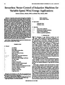
In (2.3.1) 𝜆 is called the co-state and each state equation is multiplied by a corresponding co-state 𝜆. According to the minimum principle, for the trajectory of control input 𝑢(𝑡) to be optimum, it must minimize the Hamiltonian for all 𝑡 ∈ [𝑡0 : 𝑡𝑓 ]. This may be expressed by (2.3.2). A visualization of the how the Hamiltonian for an optimal control differs from that of a non-optimal control is provided using Figure. 2.1.
9
H x* t , u * t , * t , t H x t , u t , t , t
Hamiltonian
Hamiltonian
Hamiltonian
Optimal
Sub-optimal
Non-optimal
Time
Time
(2.3.2)
Time
Figure 2.1. Visualizaing the minimum principle The minimum principle given in (2.3.2) is for control inputs 𝑢(𝑡) that have constraints (are bounded). However, this principle can also be applied for unconstrained control inputs. Hence, we have the condition that the partial derivative of the Hamiltonian w.r.t. 𝑢(𝑡) should be equal to zero given by (2.3.3). Also, to guarantee that 𝑢∗ (𝑡) indeed minimizes the Hamiltonian, the second variation of the Hamiltonian w.r.t. 𝑢(𝑡) should be greater than zero as shown in (2.3.4).
H x* t , u * t , * t , t
0 u 2 H x* t , u * t , * t , t 0 u 2
(2.3.3)
(2.3.4)
In addition to the above optimality condition, the state equation (2.3.5) must also be satisfied. Note that the state equation (2.3.5) would turn out to be the same as the state equation in (2.2.1). The dynamics of the co-state 𝜆 can be found through the co-state equation given by (2.3.6).
10
* * * dx H x t , u t , t , t dt
(2.3.5)
H x* t , u * t , * t , t d dt x
(2.3.6)
The terminal cost function 𝜙 (𝑥(𝑡𝑓 )) can be introduced into the solution process by using the tansversality condition to calculate the boundary condition for the co-states 𝜆 as given by (2.3.7).
t f
x t f
(2.3.7)
x
To reiterate, using the minimum principle of optimal control theory, finding the optimal control 𝑢∗ (𝑡) during the time 𝑡0 to 𝑡𝑓 becomes just a problem of finding the corresponding control variable 𝑢(𝑡) that minimizes (or maximizes) the Hamiltonian. For simple systems this may be possible through visual inspection of the Hamiltonian as has been demonstrated in [1]. However, for non-linear multi-state systems solutions based on visual inspection is not a feasible exercise. Only numerical methods can be used in such cases. Finally, an important property of the Hamiltonian that must be kept in mind is as follows. If the Hamiltonian is not an explicit function of time, then its value is constant at all points on the optimal trajectory given by (2.3.8).
H x* t , u* t , * t c1 2.4
(2.3.8)
Summary This chapter discussed the Dynamic Optimization based on optimal control concepts
and how it differs from optimization solutions based on calculus of variations. A brief
11
overview of the state equations and cost functional was provided. The use of Optimal Control theory was discussed. Finally, Pontryagin’s Minimum Principle and the associated necessary conditions were explained.
12
3
ELECTRO MECHANICAL ENERGY CONVERSION
Human society takes for granted its ability to harness and utilize mechanical power from sources other than what is available from our bodies. Whether it be in mundane applications like an automobile or remarkable feat like drilling tunnels under the ocean, this concept has been one of the cornerstones of human civilization. Humanity’s first source of mechanical power were domesticated animals, and they continued to be the primary sources of energy until the advent of the steam turbine in the 1st half of the 19th century. However, it was the concept of electro-mechanical energy conversion using electric motors and generators (collectively referred to as electric machines) that brought about a paradigm shift. Before the advent of electric machines, mechanical power could only be transmitted using couplings, gears, belts, or fluids (compressed air, oil), limiting the maximum distance between the power source and the application. But electric machines enabled mechanical power to be available on demand with the throw of a switch, with electrical power being supplied through metal conductors. Suffice it to say that electric machines revolutionized human society in unforeseen ways. 3.1
Features of Electric Machines Electric machines can be broadly divided into two types, namely machines that work
on Direct Current (DC), and machines that work on Alternating Current (AC). Within these two types of machines there are further classifications. However, all electric
13
machines share certain common features irrespective of their type and their widespread acceptability. The common features are: a) Rotary motion: Electric machines produce mechanical power in the form of smooth rotational motion which may be measured in terms of angular velocity, and torque (moment of force). Comparatively, steam engines produce a reciprocating motion which must be converted to a rotary motion through additional components. b) High efficiency: The conversion efficiency from electrical energy to mechanical energy and vice versa is usually in the range of 80 to 95% at the rated power of the machine. Comparatively, the maximum efficiency of a diesel engine is only about 35%. c) Controllability: By controlling the magnitude and/or the frequency of the electric current of electric machines it is possible to precisely regulate or throttle the speed/torque output of an electric machine. d) Ruggedness: There are very few moving parts in an electric machine resulting in less wear and tear, low maintenance, and machine lifetime’s exceeding 30 years. There are significant differences among the electric machines. A graphical overview of different motor types can be found in [3]. Table 3.1 lists the relative differences among the most common types of electric machines, and their common application areas. Table 3.1.Comparison of electric machine types. Type Maximum power rating
Permanent Magnet DC Motor Medium
AC Induction High
14
AC Synchronous High
Stepper Motor Low
Starting torque capability Efficiency Maintenance Capital Cost Operating complexity Speed control complexity Application
High
Medium
Medium
High
Medium High Low Low
Medium Very Low Low Low
High Low High Medium
Medium Medium Medium High
Low
Medium
Medium
High
Drones, robotics, cooling fans, toys, and engine starters
Industry+ commercial, electric cars, wind turbine generators
Power generation, electric cars, wind turbine generators
Robotics, actuators
Note that there are a few other distinct electric machine types like switched reluctance machine and DC series motor which have not been listed in Table 3.1. It can be noted from Table 3.1 that certain machine types have found a niche in certain applications. One example is the permanent magnet DC motors which are exclusively used in toys and drones, and the stepper motors in robotics. Another important fact that must be pointed out is that two types of electrical machine account for nearly 100 % of the mechanical and electric power generated in the world. All the conventional power generation plants exclusively use AC Synchronous generators. The power ratings of these machines range from a few kilowatts (Kw) in case of portable generator sets (gensets) to more than 600 Megawatts (MW) in case of steam turbine generators in electric power plants. Conversely, nearly 70% of the power generated by the AC Synchronous machines are consumed by the AC Induction motors to produce mechanical power in industrial, commercial, and domestic application. They can be found in everything from refrigerators, and air conditioning systems to industrial conveyors, and electric cars.
15
The design of an optimal control system for the AC Induction machine is the focus of this dissertation report. 3.2
Energy efficiency in electric machines A consequence of the Second law of Thermodynamics is that conversion of energy
from one form of energy to another is not 100% efficient. Electro-mechanical energy conversion systems are no exception. A fraction of electrical/mechanical power input is wasted as heat in electric machines. Depending on the measurements available, energy efficiency of an electric machine may be calculated in two ways. If the electrical machine is motoring, i.e. converting electrical energy into mechanical energy, the efficiency is calculated using (3.2.1) or (3.2.2). In case the machine is generating power, i.e. converting mechanical energy into electrical energy, the energy efficiency may be calculated using (3.2.3) or (3.2.4).
mot
mot mot
mech Eout elect Ein Eout Eout Eloss
(3.2.1)
(3.2.2)
elect Eout mech Ein
gen
(3.2.3)
Ein Eloss Ein
(3.2.4)
where 𝐸𝑜𝑢𝑡 is the mechanical energy output, 𝐸𝑖𝑛 is the electrical energy input, and 𝐸𝑙𝑜𝑠𝑠 is the energy losses in the machine over a time interval.
16
Electro-mechanical energy conversion systems, i.e. electric machines, are considerably more efficient than the thermochemical–mechanical or mechanicalmechanical energy conversion systems. Electric machines outnumber other energy conversion systems, both in quantity and operating time, and hence even small power losses add up over time to become significant energy losses. Conversely, even a couple of percentage points of improvement in energy efficiency of electric machines can lead to large energy savings over time. Energy efficiency of an electric machine (or any other energy conversion device) is not a static quantity. It is a function of state variables, input variables, and external disturbances related to the machine. Energy efficiency of an electric machine can take any value from zero to a maximum theoretical efficiency (below 100%). Also, it is highly dependent on the speed-torque output from the machine. 3.3
Maximizing Energy Efficiency Improving the efficiency (or reducing losses) of an electro-mechanical energy
conversion system is ultimately an engineering optimization problem, consisting of a cost function to be minimized (or maximized) and a set of constraints. This problem can be approached using all three methodologies mentioned in Chapter I. These are discussed as follows: a) Optimize design parameters: Select electric machine parameters like resistance, inductance, number of windings, grade of steel used in the stator/rotor, type of metal used in windings, etc. to obtain maximum energy efficiency at a specific speed-torque operating point (usually the rated speed and torque operating point).
17
b) Optimize operation during steady state: Modify state variables of the electric machine like electro-magnetic flux or stator electric current after it has reached a steady state, and maximize the efficiency at its present speed and torque operating point. c) Optimize operation during transients: Modify state variables of the electric machine like electro-magnetic flux or stator electric current while it is accelerating or decelerating to a new speed-torque operating point in such a way that its efficiency during those transitions is maximized. It is easy to observe how (a) above fundamentally differs from (b) and (c) in terms of the engineering work involved. However, from the point of view of an optimization algorithm, (a) and (b) are static optimization problems and would use similar techniques to solve. On the other hand, (c) is a dynamic optimization problem and would need a considerably different approach. As mentioned in Chapter I, this dissertation is about dynamic optimization as it exclusively focuses on optimizing induction machine operation during transients (acceleration and deceleration). Since the dynamics governing the operation of each electric machine is different, dynamic optimization problems and their solutions for different electric machines will be distinct. This work focuses entirely on the problem of improving the efficiency (or reducing energy losses) of the induction machine during its acceleration and deceleration (transient) states. 3.4
Importance of Transient Energy Efficiency in Induction Machines In most IM applications, the operating points (rotor speed and torque) remain
constant for most of its operating time (also referred to as duty cycle). For example, the rotor speed may change once every hour on average in a refrigerator application. This means that only a small fraction of the IM’s duty cycle is in transient state. For this 18
reason, improving transient energy efficiency will have only a marginal impact on the overall energy efficiency and hence has never received much interest from researchers. But in recent years IM’s have found application in electric vehicles (EV) [4], wind turbine generators [5], and fly wheel energy storage [6]. In these applications, for a significant fraction of the operating time, the IM is in a transient state because the operating point changes rapidly. In case of EV’s this is apparent from the US EPA sample drive schedules for vehicles that can be found in [7]. Hence while the objective of this thesis is applicable to IM’s in all applications, the best results would be obtained in applications with frequent speed transients. A simple illustration of the potential electrical energy savings in EV’s is given here. Assume that a 2% improvement in drive cycle energy efficiency is achieved by using transient loss minimization algorithms within the EV drive train control software. This would translate to a 2% decrease in the specific energy consumptions (kWh per mile). The resulting energy savings for different Tesla models are shown in Table 3.1. Note that Tesla exclusive uses IM’s in all their EV models. The number of Tesla vehicles on road around the world was about 200,000 in 2017 [8]. However, it is expected to reach 1 million vehicles in a couple of years and keep increasing for the near future [9]. Hence even a 2% improvement can lead to saving of millions of units of electrical energy. Table 3.2 Potential energy savings in Tesla EV's Model
EPA range (Miles)
Battery capacity (kWh)
Tesla Model S 75D Tesla Model X 75D Tesla Model 3
259 237 215
75 75 60*
Specific energy per mile (kWh/mile) 0.306 0.32 0.233
19
2% Energy Energy Saving Saving for (kWh/mile) 100000 miles (kWh) 0.0061 579 0.0063 633 0.0047 558
3.5
Summary This chapter discussed the importance of electro-mechanical energy conversion using
electric machines. It specifically highlighted the importance of induction machines. The concept of energy conversion efficiency was discussed. Different levels at which the electric machine operation can be optimized to maximize its energy conversion efficiency were described.
4
INDUCTION MACHINES
Invention of the first practical induction machine (IM) can be attributed to Nikola Tesla in 1887 and Galileo Ferraris in 1885 (both working independently). The operating principle of an induction machine was first explained by Tesla in his paper “A New System for Alternating Current Motors and Transformers”. However, it was Michael Dolivo-Dobrowolsky who perfected the design of Tesla and Ferraris and invented the most common type of induction machine being used today, namely the 3-phase Squirrel Cage induction machine (SQIM). This design has been optimized over the last 100 years, and has been the subject of many volumes of research [10], [11]. A brief explanation of the IM operation is provided below for completeness. 4.1
Induction Machine Operation It is known that when electric current flows through a closed loop wire, a magnetic
field is established that surrounds the current carrying loop of wire. Now, when a magnetic field and a conductor moving at relative speeds w.r.t. each other intersect, a voltage (also referred to as the electromotive force (emf)) is induced across the conductor 20
(Faraday’s law of induction). If the conductor is short circuited, i.e. forms a loop, the induced emf causes a current to flow through it. The direction of this current is in such a way that the magnetic field it produces will be in the opposition to the magnetic field that caused it in the first place (Lenz’s law). If the magnetic field is moving and the metal conductor is stationary (as in the case of an IM), the induced current interacts with the magnetic field (Lorentz’s force law) to produce a force that acts on the conductor and causes the conductor to move in the direction of the magnetic field.
Stator Core (Steel)
Short Circuited Metal Conductors (Aluminium or Copper)
Stator Windings (Copper)
Φ1
3 phase sinusoidal voltage waveforms Φ2
Φ3
Rotor Core (Steel)
Rotor Shaft Air Gap between Rotor and Stator
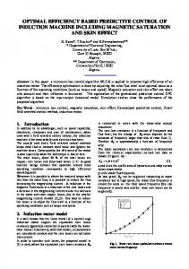
Figure 4.1. Induction machine cross sectional diagram. An IM has primarily two major components as illustrated in Figure 4.1, namely the stator and the rotor. The stator consists of three coils of insulated copper wires and are physically displaced by 120 degrees on the stator. This three-coil arrangement is known as the stator winding. The terminals of each of the three stator windings are supplied with a sinusoidal voltage waveform. The three sinusoidal voltage waveforms are themselves
21
phase displaced from each other by 120 degrees and when applied to the stator windings will produce a rotating magnetic field (RMF). The RMF links with the rotor conductors through the air gap (a clearance between the rotor and the stator). The rotor core consists of insulated metal discs called laminations fixed around a shaft that is free to rotate about its axis. Embedded with these laminations are short-circuited metal conductors. The current induced in the rotor interacts with the RMF to produce a torque that causes the rotor structure to spin and catch up with the RMF, thereby reducing the relative speed between them. Hence, all the energy transfer that occurs between the stator and rotor is through the electro-magnetic linkage through the air gap. The speed at which the RMF rotates is known as the synchronous speed, 𝑁𝑠𝑦𝑛𝑐ℎ and is given by (4.1.1), if measured in revolutions per minute (RPM).
N sync
120 f p
(4.1.1)
where 𝑓 is the frequency of the sinusoidal voltage waveforms being supplied to the stator windings, and 𝑝 is the number of stator magnetic poles that result from stator windings. The rotor speed, 𝑁𝑟 , can never reach the synchronous speed of the stator magnetic field. If 𝑁𝑟 were to become equal to 𝑁𝑠𝑦𝑛𝑐 then the relative speed between the stator magnetic field and the rotor conductors would become zero thereby preventing emf from being induced (Faraday’s law), current from flowing (Lenz’s law), and consequently torque becoming zero. The relative difference between rotor speed and the RMF’s synchronous speed is known as the slip of the machine and is calculated using (4.1.2). More importantly, slip is a measure of the magnitude of current that flows in the rotor
22
conductors, as well as the amount of electro-magnetic torque that is being produced. The value of slip typically varies from 0.1% to 5%.
s
4.2
N sync N r
(4.1.2)
N sync Induction Machine Drives
In many industrial applications precision control of speed and torque is necessary, i.e. the machine’s speed is expected to change depending upon the need of the application at that time. An old example is the HVAC systems in buildings, while electric cars are a new example. Speed control over a limited range is possible through the use of gears, however, these would add complexity and energy losses to the system. From (4.1.1) and (4.1.2), speed control is possible by changing the frequency of the stator’s sinusoidal voltage waveform. However, changing the supply frequency is not a trivial task, and for this reason DC motors were the favored machines for such speed control applications until the latter half of the 20th century. However, the advances in power electronics technology made it possible to have precise control over the magnitude, frequency, and phase of the voltage waveform supplied to the stator of the IM even at high current and voltage levels for a reasonable price and complexity. The power electronic devices that convert DC waveforms to sinusoidal AC waveforms required by AC machines are called 3-phase inverters. A simple description for these are: circuits comprised of on/off electronic switches which can be controlled independently with one side connected to a DC voltage source and other side connected to the AC machine. The switches are functionally like a normal mechanical switch except that they can be turned on and off thousands of times every 23
second continuously with minimal power losses. Also, these switches can carry very large currents without damage if sufficient heat dissipation is provided. Through operating the switches in a precise and specific sequence and duty cycles, the desired voltage waveforms with a desired frequency can be generated. The inverter, IM, and the software algorithms are collectively referred to as the IM drive. References like [12] discuss IM and other electric drives in detail. The schematic of a generic IM electric drive system is shown in Figure 4.2. Frequency-Voltage Controlled Waveform
DC Voltage Waveform
60 Hz AC Voltage Waveform
3-ph Power Electronic Inverter
AC to DC Converter
IM
User Interface Switching signals Software
Voltage/Current Controllers
Switching Hardware
Switching Logic
Figure 4.2. IM Electric Drive Schematic 4.3
Induction Machine Power Flow and Power/Energy Losses A graphical illustration of the power flows and relative differences in magnitude
between power/energy losses in an induction machine are given in Figure. 4.3 and Figure. 4.4, respectively.
24
Ohmic Loss
Ohmic Loss
Magnetic Flux Linkage
Rotor
Energy stored in Rotor Mass
Core Loss
Stator
Energy stored in Magnetic field
Electrical Power
Friction Loss
Mechanical Power
Core Loss
Figure 4.3. Power flows in an induction machine Energy stored in Magnetic field Core Loss (Hysterisis & Eddy current)
Ohmic Loss in stator and rotor
Mechanical Power
Kinectic Energy in Rotor Mass
Windage + Friction Loss
Figure 4.4. Relative magnitude of Power flows in an induction machine Electrical power that the source supplies to an IM is transformed in three ways. 1) Mechanical power: Most of the input electric power is transformed into output mechanical power at the rotor. This output mechanical power is a function of the torque of the load connected to the motor shaft and the rotor speed. It can be 25
expressed as (4.3.1). A small fraction of the mechanical power is lost due to friction in the bearings that support the rotor shaft. Another fraction is lost due to drag offered by air due to the rotation of the shaft. These losses are functions of the rotor speed (4.3.2). Another fraction of the output mechanical power is stored as kinetic energy (4.3.3) in the rotating mass of the rotor. Note that transfer of power to the rotor mass occurs only when rotor speed is increasing. If the rotor speed were to decrease, the kinetic energy is released as the mechanical output of the rotor. No energy is transferred to the rotor mass when rotor speed reaches steady state.
Pmech TLr
(4.3.1)
Pfriction/ windage f r 1 Estored J r2 2
(4.3.2) (4.3.3)
In the above equations 𝑇𝐿 is the load torque on the rotor shaft, 𝜔𝑟 is the rotor mechanical speed, and 𝐽 is the moment of inertia of the rotor mass. Every speed-torque operating point has a corresponding mechanical power output. Hence these are hard constraints for the energy efficiency optimization problem. Since the friction, and windage losses are fixed for a specific speed-torque operating point, these are considered as uncontrollable energy losses and not part of the optimization problem. 2) Ohmic losses: When electric current passes through any type of conductor heat is generated which can be expressed as (4.3.4). In case of an IM, Ohmic losses occur when current flows through the stator windings and the short-circuited rotor conductors. 26
Pohmic i 2 R
(4.3.4)
where 𝑖 is the current flowing through the conductors, and 𝑅 is the resistance of the conductors. Since electric current is a controllable input to the IM, Ohmic losses can be considered as controllable losses and part of the optimization problem to maximize energy efficiency. 3) Electromagnetic flux: A explained earlier, a rotating magnetic field is produced due to the sinusoidal currents flowing through the stator windings. The magnetic flux flows through the stator core, air-gap, and rotor core. Some of the input electrical energy is stored in the magnetic field. The amount of energy stored is a function of the current flowing through the stator windings. The flow of magnetic flux through the metal that constitutes the core of the stator and the rotor also results in two types of energy losses: eddy current losses and hysteresis losses. These losses are expressed by (4.3.5) and (4.3.6), respectively. These losses are collectively referred to as core or iron losses.
Peddy Ke K f Bm2 f 2 Physterisis Kh Bm1.6 f
(4.3.5) (4.3.6)
where 𝐵𝑚 and 𝑓 are the peak magnetic flux and the frequency at which the magnetic poles change on the stator, respectively. 𝐵𝑚 is proportional to the magnitude of the sinusoidal voltage waveform, while 𝑓 is equal to the frequency of the same. 𝐾𝑒 , 𝐾𝑓 , and 𝐾ℎ are constants related to the type, volume, and the shape of material used to construct the stator and rotor cores.
27
Since the functions describing core losses have two degrees of freedom, the core losses can be considered as controllable losses and hence part of the optimization problem. 4.4
Induction Machine Dynamics Like all dynamical systems, the operating cycle of an IM can be separated into
transient and steady state phases. An induction machine is said to be in steady state if its rotor speed, electromagnetic torque, magnitude of the voltage and current waveforms, and peak magnetic flux remain constant. The IM can be induced into a transient phase from steady state in two ways as listed below: a) Change in the frequency or the magnitude of input sinusoidal voltage waveforms. b) Change in the load torque on the shaft. Transients can also be caused due to short circuits or open circuits in the stator or rotor windings. These are outside the scope of this dissertation, and hence not discussed. The most common transient that occurs in IM is when the machine accelerates or decelerates from its current speed to a higher or lower speed, respectively. As with other dynamical systems, transients in IM can lead to two possibilities. a) IM achieves a new steady state operating point. The simplest example of this is an IM increasing its rotor speed to a new operating point in response to a change in input voltage magnitude and frequency. b) IM becomes unstable which may lead to stalling, over speeding, or overheating.
28
The most common example of instability is when the load torque on the IM is suddenly increased to a value that is beyond its maximum torque rating. This results in the net torque becoming negative, and the machine coming to a stop (stalling). Figure 4.5. Illustrates a transient in the input phase voltages of an IM. It can be observed that the magnitude and frequency of the voltage waveforms for all three phases change at 0.5s, 1s, and 2s. The transient phase that follows is highlighted using the circles.
Voltage (V)
500 0 0
0.5
1
-500
1.5
2
2.5
3
2
2.5
3
2
2.5
3
Time (s)
Voltage (V)
500 0 0
0.5
1
-500
1.5 Time (s)
Voltage (V)
500 0 0 -500
0.5
1
1.5 Time (s)
Figure 4.5. Transients in input phase voltage waveforms of an induction machine. The change in input voltage corresponds to a change in the rotor speed as shown in Figure 4.6. A steady state phase follows each of the transients. There is a difference in the magnitude of the power/energy that is consumed by the IM during transients and steady
29
states. This is illustrated in Figure 4.7. by plotting the cumulative energy input into the IM during the above transients.
Speed (rad/s)
145
95
Rotor Speed
45
-5
0
0.5
1
1.5
2
2.5
3
Time (s) Figure 4.6. Transients and steady states in rotor speed of IM corresponding to voltage transients 9000 8000
Energy Input
7000
Energy
6000 5000 4000 3000 2000 1000 0 0
0.5
1
1.5
Time (s)
2
2.5
3
Figure 4.7. Transients & steady states in energy input to IM corresponding to voltage transients Most of the input energy consumed during transients is used to accelerate the IM to its new speed-torque operating point while the rest is consumed by the energy losses that
30
were described earlier. Details on how the dynamics of the IM affect the energy input and the energy losses will be explained in the Methodology section of this dissertation. 4.5
Mathematical Modelling of Induction Machines The dynamics of an IM can be described through a system of ordinary differential
equations (ODE’s). In one approach, the model is built around treating the three phase variables as they are. That is, there is no transformation of the variables. In such an approach, there will be 3 variables representing the current, voltage, and the magnetic flux linkage of each phase of the IM. Also, the mutual inductance of the IM, which is a coefficient in the ODE’s, would be a function of the rotor speed. Hence, we arrive at a time variant model of the IM consisting of 3 input variables, 7 state variables, and 6 dependent variables. Fortunately, there is a second approach that can yield a significantly simpler model without losing accuracy of the model. This involves transforming the three a, b, and c phase variables into two d and q phase variables by projecting them onto the orthogonal d- and q-axes of a rotating reference frame [13]. Apart from reducing the number of variables, the transformation of variables also results in the mutual inductance becoming independent of the rotor speed, i.e. it becomes a constant. The transformation from 3 phase variables to 2 phase variables is called Park’s transform. The speed of the rotating reference frame can be arbitrarily chosen, and the properties of the IM model varies accordingly. The concept is illustrated in Figure 4.8.
31
A Park’s transform
Figure 4.8. Visualizing change in reference frame In this dissertation, the reference frame speed is chosen to be equal to the frequency of the input voltage waveforms of the stator. Using magnetic flux linkages as the state variables, the transformation of variables results in an ODE model of the IM as given by (4.5.1) to (4.5.5) [14], [15].
d ds vds Rs ids sync qs dt d qs vqs Rs iqs sync ds dt d dr vdr Rr idr sync r qr dt d qr vqr Rr iqr sync r dr dt p i dr iqr TL dr p 2 qr dr dt 2 J
(4.5.1)
(4.5.2) (4.5.3)
(4.5.4)
pLm i qr ids TL p 2 Lr dr qs J 2
(4.5.5) where 𝛹𝑑𝑠 and 𝛹𝑞𝑠 are the stator flux linkages along the new d-axis and q-axis, respectively. 𝛹𝑑𝑟 and 𝛹𝑞𝑟 are the rotor flux linkages along d-axis and q-axis, respectively. 𝑖𝑑𝑠 and 𝑖𝑞𝑠 are the stator currents along d-axis and q-axis, respectively. 𝑖𝑑𝑟 and 𝑖𝑞𝑟 are the rotor currents along d-axis and q-axis, respectively. 𝑣𝑑𝑠 and 𝑣𝑞𝑠 are the stator input voltage along d-axis and q-axis, respectively. 𝑣𝑑𝑟 and 𝑣𝑞𝑟 are the rotor input 32
voltage along d-axis and q-axis, respectively. 𝑅𝑠 and 𝑅𝑟 are the resistances of the stator and rotor windings, respectively. 𝜔𝑠𝑦𝑛𝑐 is the frequency of the source voltage waveforms at the stator and 𝜔𝑟 is the rotor speed. 𝑇𝐿 is the load torque on the rotor (torque in opposition to rotation of the rotor) while 𝐽 is the moment of inertia of the rotor. Finally, 𝑝 denotes the number of magnetic poles due to the stator windings. In most IM’s the rotor windings are short circuited, hence 𝑣𝑞𝑟 = 𝑣𝑑𝑟 = 0. The rotor currents can be expressed as functions of stator currents, and the rotor flux linkages can be expressed through the algebraic relationships given by (4.5.6) to (4.5.9) [15].
idr
iqr
ds Ls ids
(4.5.6)
Lm qs Ls iqs
(4.5.7)
Lm Lmids idr dr Lr Lmiqs iqr qr Lr
(4.5.8)
(4.5.9)
where 𝐿𝑠 is the stator inductance, 𝐿𝑟 is the rotor inductance, and 𝐿𝑚 is the mutual inductance. 4.6
Current Fed Model of The Induction Machine The mathematical model in section 4.5 used stator input voltages as control inputs
and hence it is known as the voltage fed model. It is also possible to use stator input currents as the control inputs and obtain a smaller model of the IM. Using currents as inputs implies that the dynamics between stator flux and stator voltages can be neglected. It is assumed that there are current controllers with very fast settling times between the
33
IM and the input voltage source that control the input voltage. Hence the dynamics of the IM only depend on the reference to the current controller. This concept is illustrated in Figure 4.9.
Vc
Icref
Vb
Ibref
Iaref
Va
Current Controller
Ib
Induction Machine
Ic Current Measurement Feed back
Figure 4.9. Concept of Current Fed IM Model Using stator current as input to the model removes the need for ODE’s involving stator flux variables, i.e. (4.5.1) and (4.5.2). Substituting the equations for rotor currents, (4.5.8) and (4.5.9) in (4.5.3) to (4.5.5) results in an IM model having 3 state variables as shown in (4.6.1) to (4.6.3).
Lmids d dr Rr dr sync r qr dt Lr d qr Lmiqs Rr qr sync r dr dt Lr
34
(4.6.1)
(4.6.2)
p dr Lmids qr Lr d r p 2 dt 2
qr Lmiqs dr TL L r J
(4.6.3)
The above model will be further simplified later in this work and used in the IM optimal control problem. 4.7
Detailed Problem Statement There is a significant scope for improving the energy efficiency of an IM during both
steady state and transient phases. Algorithms for minimizing energy losses during steady state are already available in commercial IM drives, whereas transient energy loss minimization algorithms are not. As such, the contribution and the objective of this work is to find an optimal control law that minimizes the Ohmic and iron energy losses inside an IM during the transient phases of operation without compromising the performance of the machine in terms of its output mechanical power. A secondary contribution and objective of this work is to determine the sensitivity of the control law to the operating conditions of the IM. Additionally, the tertiary objective is that the designed control law must be in a form that allows it to be incorporated into the existing IM drive control algorithms. 4.8
Summary This chapter briefly explained the operation of, the power flow through, and the
various power losses within an IM. The transient phase of the machine was discussed. The ODE representation of the IM model was given. Finally, a more detailed overview of the research problem that is addressed in this work was provided. 35
5
LITERATURE SURVEY
Optimal control is a fascinating optimization technique and its development history, which began about 300 years ago, is equally fascinating. Its relationship to mathematics, engineering, and computer science is illustrated in Figure 5.1.
Mathematics
Calculus
Optimal Control
Optimal Control
Figure 5.1. Relationship between optimal control and other technical areas 5.1
History of Optimal Control The excellent historical overview provided by Sussmann et al. in [16] describes the
inception of optimal control theory through a mathematical challenge put forward by Johann Bernoulli in 1696 in the form of the Brachystochrone problem. The authors of [16] also present their solution to the said problem using the optimal control approach, and showed how it was superior to the Calculus of Variations solution. A few other notable works chronicling the history of optimal control are [17], [18], and [19]. The 36
development of the Euler-Lagrange equation was a key discovery in the advancement of Calculus of Variations. However, it was the efforts of two cold war era mathematicians, Lev Pontryagin in the Soviet Union and Richard Bellman in the US that established optimal control theory as a new field in applied mathematics, and distinguished it from Calculus of Variations. A timeline has been created illustrating the major developments in the field by extracting relevant information from the above-mentioned references, and shown in Figure 5.2.
1696
Brachystochrone Problem
Leonard Eule & Joseph Lagrange
1744 to 1755
Calculus of Variations and Euler-Lagrange equation
AM Legendre
1786 1834
WR Hamilton Karl Weierstrass
Second Variations (Legendre–Clebsch condition) Hamiltonian function
1879
Calculus of Variations era
Johann Bernoulli
Weierstrass condition
1956
Richard Bellman
1957
RE Kalman
1960
Linear Quadratic Regulator
IM Ross
2000's
Pseudo-Spectral optimal control
Optimal Control Theory
Pontryagin’s maximum principle Dynamic programming (Bellman equation)
Lev Pontryagin
Figure 5.2. Optimal Control through history Pontryagin’s discovery of the Maximum principle paved the way for control engineers to solve optimal control problems involving continuous variables in a more 37
intuitive way compared to using Calculus of Variations. Bellman was responsible for the development of dynamic programming, which made it possible to solve piecewise optimal control problems [20]. The development of the Linear Quadratic Regulator by Kalman using the minimum principle enabled practically implementable optimal controllers for linear systems [21], [22]. The work of this dissertation uses Pontryagin’s maximum principle to define a set of necessary conditions and use them to develop an optimal control law for minimizing transient energy losses in an accelerating IM. 5.2
Literature on transient energy loss minimization in IM’s The problems involving optimizing the IM operation during steady state in real time
is a heavily researched topic compared to optimizing during transient states. An excellent survey of the various techniques used for IM steady state optimization over the past 15 years is given in [23]. There have been several researchers who have attempted to solve the research problem of optimizing IM operation during transients, but there has yet to be a survey that chronicles their efforts. This section will provide a brief outline on the efforts of all the researchers over the last 40 years who have worked on this research problem. A chronological illustration is provided in Figure. 5.3. Note that the survey includes papers from both conferences and journals.
38
1968 1984 1988 1990 1991 1992 1999 2002
Petrov [24] Figalli [25] Sangwongwanich [29,30], Lorenz [26] Murata [33] Sangwongwanich [31-32] Lorenz [27,28] De Wit [34] Rodriguez [35]
2006
Gonzalez [36]
2007
Inoue [38]
2008 2009
Botan [37] Gaicenau [42]
2010 2011
Rosu [43], Ali [45] Inoue [39]
2012 2013 2015 2016
Inoue [40] Stumper [46,47], Gaiceanu [44], Inoue [41] Plathottam [49] Weis[48], Plathottam [50], Borisevich [51]
Figure 5.3. Dynamic optimization in Induction Machines Literature The concept of using optimal control theory in electric machine control applications can be traced back to the work of a Soviet engineer named Petrov in [24]. He developed control trajectories for DC series motor, DC permanent magnet motor, and the induction motor using optimal control principles. However, he only considered stator transient Ohmic losses, used a very simple model, and used control variables that made it impractical to implement with modern power electronic drives. The work by Figalli in [25] during early 1980’s was the first to use Bellman’s equation to develop an optimal control law for frequency of the IM with objective to reduce speed error and control effort. The subject did not receive much attention until the early 1990’s. The work by 39
Lorenz in [26]–[28] again proposed to use Bellman’s equations from Dynamic programming to solve the transient energy loss problem, considering both stator and rotor Ohmic losses as well as core losses. This was also the first work to use d- & q-axis currents as control inputs in the transient energy loss minimization problem. This solution was compatible with power electronic drives using the Field Oriented Control algorithm. However, the Bellman equations resulted in the need to solve partial differential equations to compute the optimal control trajectories. Hence, trajectories were computed offline and stored as a lookup table on the controller. This technique could only be used if all possible load torque values and speed reference values encountered in the IM duty cycle were available before hand, thereby limiting its practical use. During the same period Sangwongwanich used Pontryagin’s minimum principle to develop a control law for the IM that minimized the time taken to increase its rotor speed [29]–[32]. It used the angle between d- and q-axis currents as the control input. However, energy losses were not considered in this work, i.e. it was purely a minimum time solution. Another work that used optimal control principles without considering transient energy losses was by Murata in [33]. The linear quadratic regulator was used for speed control with stator currents as the control inputs. In the late 1990’s the work by De Wit in [34] used the Euler-Lagrange equation to derive a set of necessary conditions to be satisfied by the optimal rotor flux trajectory in a field oriented control of an induction machine. Stator and rotor Ohmic losses were considered in the cost function. This work treated the problem like a Calculus of Variations problem rather than an optimal control one. However, unlike the earlier works,
40
they gave no simulation or hardware results to show the feasibility of their optimal rotor flux trajectory solutions. During the early 2000’s the work by Rodriquez in [35] and Gonzalez in [36] used Pontryagin’s minimum principle for obtaining the maximum torque per current input. However, their cost functional didn’t have any power loss terms or terminal costs. Hence, they could find an equation for the optimal d- and q-axis current trajectories (as control inputs). The parameter’s in their analytical equation took on different values for different initial and final conditions. Hence, they had to be computed offline and stored as a lookup table in the controller. The work by Botan in [37] also used the minimum principle, a cost function with stator and rotor Ohmic losses, and the stator d- and q-axis currents as control inputs. However, the fact that they considered only the rotor speed dynamics makes the validity of their optimal trajectory debatable. The work by Inoue in [38] used the Euler-Lagrange equation to find the optimal torque trajectory that maximizes regenerative power. In early 2010 the same concept was used again by the same authors in [39]–[41] for minimizing stator and rotor Ohmic losses during transients. During the same time period the work by Gaiceanu and Rosu in [42]–[44] used a linear quadratic regulator for speed control and for minimizing the stator Ohmic losses. They calculated the optimal trajectory of the stator q-axis current online using the Matrix Riccati Differential Equation (MRDE). This is a good approach for practical implementation except that only the Ohmic losses due to stator q-axis current are considered. Another work that used the Bellman equation to minimize stator and rotor Ohmic losses was by Ali in [45]. Unlike the work by Lorenz, Ali found the optimal flux trajectory as an offline solution, instead of the optimal stator current, and then fitted a
41
polynomial curve to reproduce the optimal flux trajectory during real time operations. However, this method was not generalized to be applicable for an arbitrary IM. The recent related works in this area (other than the work of the author of this dissertation) are by Stumper [46], [47] in 2013 and Weis [48] in 2016, both of which extended De Wit’s work. Stumper’s work used the Euler-Lagrange equation to come-up with a predetermined torque trajectory to find the optimal rotor d-axis flux trajectory that minimized Ohmic and eddy current losses during torque transients. The distinguishing feature of Stumper’s work was the development of a closed form equation for the optimal rotor d-axis flux trajectory which took the shape of a first order lag. However, the problem with this optimal trajectory was that it assumed speed was constant during the torque transients. Hence, it was not optimal for an IM that is accelerating from one speed to another. The next work in this area was by the author of this dissertation in [49] and [50] in 2015 and 2016, respectively. Weis [48] extended the work of Stumper, but did not assume speed was constant during transients. He found that the optimal rotor flux trajectory in an accelerating IM could be described by a conic section. Concurrently, the same conclusion was arrived at by the author of this dissertation in [50]. Since both Stumper and Weis treated it as a Calculus of variation problem, they found the optimal state trajectory instead of the optimal control trajectory. The most latest work in this area just before the writing of this dissertation was by Borisevich [51]. He set up an optimal control problem to minimize stator and rotor ohmic losses, but only considered the flux dynamics since he assumed a predetermined trajectory for the electromagnetic torque (like Stumper). Borisevich also derived some necessary conditions using Pontryagin’s minimum principle but did not solve them numerically. Instead, using some
42
simplifications he was able to express the stator d-axis current in terms of the q-axis current (which was known due to the pre-determined torque trajectory). However, no analysis was done on the shape of these trajectories. The above surveyed literature has been classified into four groups depending on the mathematical technique used as illustrated in Figure 5.4. The different techniques used to generate the optimal control trajectories of IM in real time are illustrated in Figure 5.5. The dynamic models, cost functions, and control inputs that have been used in the surveyed literature are tabulated in Table 5.1.
Euler-Lagrange Equation [24], [34],[38-41], [46-47],[48]
Dynamic Programming [25],[26-28],[45] Dynamic Optimization in Induction Machine
Linear Quadratic Regulator [33], [42-44]
Pontryagins Minimum Principle [29-32], [35-36],[37], [49-50],[51]
Figure 5.4. Dynamic optimization in Induction Machines in Literature
43
Real Time Implementation
Neural Networks
Ricatti Equation
Look up table
Iterative
Computational Complexity Figure 5.5. Different techniques used to generate the optimal control trajectories of IM Table 5.1. Comparing literature on transient energy loss minimization in induction machines Reference
Energy cost
Petrov Lorenz
Sangwongwanic h
De Wit
Rodriguez, Gonzalez
Operatin g point cost None
State variable
Control input
Solution
Rotor Ohmic loss Stator + None rotor Ohmic, eddy current + hysteresis losses None Minimum time
Stator flux, rotor speed Rotor daxis flux, Rotor speed
Frequency , Voltage Stator dand q-axis current
NA
Rotor daxis flux, Rotor speed
Algebraic equation
Stator + rotor Ohmic losses, Stored magnetic energy Stator Ohmic losses
None
Rotor dand q-axis flux
Phase angle of stator current vector Stator dand q-axis currents
Minimum time
Rotor magnetizin g current, rotor speed
Stator dand q-axis currents
Algebraic equation
44
Look up table
NA
Inoue
Botan
Ali
Gaiceanu
Stumper
Plathottam
Weis
5.3
Regenerativ e braking power Stator + rotor Ohmic losses, Stator + rotor Ohmic losses
None
Rotor speed
Optimal torque
Algebraic equation
None
Rotor speed
Algebraic equation
None
Stator Ohmic losses (qaxis current) Stator + rotor Ohmic losses, Eddy current losses Stator + rotor Ohmic losses, Eddy current losses
Speed error
Rotor dand q-axis flux, Rotor speed Rotor speed
Stator dand q-axis currents Stator dand q-axis currents Stator qaxis current
Riccati
Stator + rotor Ohmic losses, Eddy current losses
Polynomia l
None
Rotor daxis flux
Rotor daxis flux
Iterative
Speed error, load torque error
Rotor daxis flux, Rotor speed
ANN
None
Rotor daxis flux
Stator daxis current, rotor qaxis current Rotor daxis flux
Iterative
Contributions of this Dissertation The distinguishing features which differentiate the work in this dissertation from
previous works are listed below: 1. This work showed that it was possible to numerically solve an IM optimal control incorporating both transient energy losses (stator ohmic, rotor ohmic, and eddy current) and steady state error (rotor speed, rotor flux, electromagnetic torque). Consequently, it was possible to minimize the energy losses as well as bring the IM to
45
its new speed-torque operating point in a specified amount of time. This is a straightforward approach compared to earlier works. Also, this work considered both the non-linear flux and speed dynamics while formulating the IM optimal control problem. In contrast, many of the other works neglected either the flux dynamics or the speed dynamics or used linearized models while formulating the optimal control problem. 2. This work is the first to generate real time optimal trajectories for stator currents using neural networks. Many works used lookup tables for entire optimal trajectories corresponding to specific initial and final conditions. Other works used open loop control laws that took different parameters depending upon the operating point of the IM. 3. This work was one of the first to propose a conic trajectory for rotor d-axis flux during IM acceleration/deceleration (Weis et al. concurrently arrived at the same conclusion). Additionally, it discovered that the optimal q-axis current could take either a conic trajectory or a constant value trajectory. The prototype trajectories were fully described in the form of analytic expression that are applicable to a generic field oriented induction machine. These expressions made it possible to perform sensitivity analysis of energy efficiency during transient which have not been done in literature before. 5.4
Summary The history of optimal control was briefly discussed and important contributions by
various mathematicians over the time were presented. All the publicly available literature on transient loss minimization in induction machines were discussed. In solving the
46
problem, it was evident from historical developments that primarily four methodologies were used and that the Euler-Lagrange equation was the most popular. The most used control inputs were stator currents, or d-axis rotor flux. Stator and rotor Ohmic losses were considered by almost all researchers. Finally, the contributions of this dissertation to the existing literature were listed.
47
6
OPTIMAL CONTROL OF DC MOTOR
To set the stage for the work of this dissertation, instead of first tackling the transient energy loss minimization problem for an IM, a similar problem for the Permanent Magnet DC (PMDC) motor is presented. Using Pontryagin’s minimum principle, the necessary conditions for an optimal trajectory are derived, from which an analytical expression for the optimal armature current is developed. 6.1
PMDC Motor Model and Cost Functional The current fed model for the permanent magnet DC motor (PMDC) is given by state
equation (6.1.1) and has rotor speed as the state variable and armature current as the control variable.
dr kia TL , r t0 rt0 dt J
(6.1.1) 𝑡
𝑘
𝑘
For simplicity, in what follows we assume 𝑇𝐿 = 𝑡0 = 𝜔𝑟0 = 0 and 𝑘1 = 𝐽 and 𝑘2 = 𝑅1 . 𝑎
The value of armature current 𝑖𝑎 that would accelerate the machine to a reference speed, 𝑟𝑒𝑓
𝜔𝑟
ia
in time 𝑡𝑓 can be calculated by (6.1.2).
rref
(6.1.2)
t f k1
However, the goal here is to minimize Ohmic losses for the DC motor during the transient period. A functional is defined in (6.1.3) that puts a cost on both the Ohmic
48
losses due to the armature resistance, and the deviation from the reference rotor speed at the end of the transient time interval. A weight 𝑤1 is assigned to the speed deviation.
J w1
ref r
r t f
tf
i t R dt 2
2 a
(6.1.3)
a
t0
6.2
Necessary Conditions using Pontryagin’s Minimum Principle Applying the Hamiltonian in (2.3.1) to (6.1.1) and (6.1.3) a new Hamiltonian is
created as in (6.2.1) from which the co-state equation (6.2.2) is then derived. The co-state equation can be integrated to obtain (6.2.3).
ki t 2 H r , ia a t ia t Ra J
(6.2.1)
d H 0 dt r t c1
(6.2.2) (6.2.3)
Using the transversality condition and the terminal cost function, the following boundary condition for the co-state is found.
t f
rref r t f w1 r
2
2w1 rref r t f
(6.2.4)
The optimal armature current 𝑖𝑎∗ (𝑡) should also satisfy the optimal control equation (6.2.5). The control input (armature current) can then be expressed in terms of the costate as in (6.2.6). Note that if we substitute (6.2.3) and (6.2.6) back into the Hamiltonian (6.2.1), it’s value becomes a constant during the transient as expected (see (2.3.6)).
H r , ia ia
k1 t 2 Ra ia t 0 49
(6.2.5)
k k ia t 2 t 2 c1 2 2
(6.2.6)
Integrate the state equation (6.1.1) and substitute (6.2.6) into that to express the rotor speed in terms of the co-state as shown in (6.2.7). Similarly, the terminal rotor speed can be expressed using (6.2.8).
k1k2 c1t 2
r t k1ia t
(6.2.7)
k1k2 c1t f 2
r t f
(6.2.8)
Using (6.2.3), (6.2.4), and (6.2.8) it is possible to obtain the condition (6.2.9), which can be solved to find the co-state 𝑐1 as in (6.2.10).
kk 2w1 rref 1 2 c1t f 2 2w1rref c1 1 w1k1k2t f
c1
(6.2.9)
(6.2.10)
c1 can now be substituted into (6.2.6) to find the value of the optimal current trajectory (6.2.11) and the terminal rotor speed corresponding to that trajectory (6.2.12).
w1k2rref ia t 1 w1k1k2t f
(6.2.11)
w1k1k2rref r t f tf 1 w1k1k2t f
(6.2.12)
Finally, by substituting (6.2.11) and (6.2.12) into the cost function (6.1.3) we get the optimal cost (6.2.13). If instead the sub-optimal value of current, as given by (6.1.2), had been used, then the cost function would have been as given in (6.2.14).
50
J opt
J nonopt
w1 rref
2
1 k1k2 w1t f rref t k f 1
(6.2.13)
rref Ra t f t f k1k2 2
2
(6.2.14)
𝐽𝑜𝑝𝑡 will always be smaller than 𝐽𝑛𝑜𝑛−𝑜𝑝𝑡 , and as 𝑤1tends to infinity, 𝐽𝑜𝑝𝑡 = 𝐽𝑛𝑜𝑛−𝑜𝑝𝑡 . The above proposed optimal control solution was tested using the DC motor specifications given in Appendix I. Table 6.1 gives the optimal current, energy cost, and current for different speed deviation weights. For comparison, Table 6.1 also gives the cost if the DC motor was accelerated using the sub-optimal current calculated through (6.1.2). As expected, these results show that the value of the optimized objective function is always smaller than that of the sub-optimal control. Also, as 𝑤1increases the optimal current converges to the same value as that of the non-optimal control. Table 6.1. Comparing optimal control and non-optimal control in PMDC Motor Weight Current (w1) (A) Optimal control 1 15.78947 2.5 16.30435 100 16.65741 Non- optimal control NA 16.67
Energy cost Terminal (J) speed (rad/s)
Speed Deviation (rad/s)
Objective function
498 94.73 531 97.82 554.938786 99.94
5.26 2.17 0.055525
526.31 543.47 555.24
555.55
0
555.55
100
The derivation of the optimal control trajectory for PMDC was an illustration of how solutions for even simple optimal control problems are neither intuitive nor trivial. 6.3
Summary This chapter presented the application of Pontryagin’s minimum principle for finding
the optimal control law for a current fed PMDC motor. 51
7
NECESSARY CONDITIONS FOR OPTIMAL CONTROL IN INDUCTION MACHINE
This chapter presents the optimal control problem formulation for IM transient loss minimization purposes. First, the rotor field oriented model is presented and sub-optimal control trajectories are analyzed. The power losses are expressed in terms of the variables in the model. Finally, the minimum principle is applied to derive the necessary conditions. 7.1
Rotor Field Oriented IM Model The current fed model of the IM in section 4.6 can be further simplified if we assume
that the entire rotor flux vector lies on the d-axis of the rotating frame of reference. This can be accomplished by manipulating the electrical frequency using (7.1.1). [15] provides a detailed explanation of the reasoning behind it. Note that this concept is used in almost all commercially available IM drives for achieving high precision speed control [52].
sync t r t
Rr Lm
Lr dr t
iqs t
(7.1.1)
With the above manipulation, the rotor flux along the q-axis of transformation would be 𝛹𝑞𝑟 = 0, and
𝑑𝛹𝑞𝑟 𝑑𝑡
= 0. Hence equations (4.6.1) to (4.6.3) may be rewritten as (7.1.2) to
(7.1.4). It can be noted that in a rotor field oriented IM the stator currents are decoupled from each other i.e. if we try to change one it will not affect the other. This allows us to have a simple control scheme to independently control rotor flux and electromagnetic torque.
52
d dr Rr Lmids t dr t dt Lr
(7.1.2)
pLm iqs t dr t TL 2 L d r p r dt 2 J 0 r t0 r , dr t0 dr0
(7.1.3)
(7.1.4)
0 where 𝛹𝑑𝑟 is the initial value of the rotor flux along the d-axis and 𝜔𝑟0 is the initial rotor
speed. In (7.1.4), 𝜔𝑟 corresponds to the rotor speed in electrical radians per second, also referred to as the electrical speed. Rotor speed can also be expressed in terms of the mechanical radians per second as shown in (7.1.5), which is referred to as the mechanical speed of the machine. Speed encoders used for measuring the rotor speed measure the mechanical speed. The mechanical power output at the rotor shaft is calculated using this mechanical speed.
m 2
r
(7.1.5)
p
From here onward all the expressions for rotor speed will be written in terms of the mechanical speed. 7.2
Analysis of the IM Model This section discusses the different trajectories that can be taken by state and control
variables of the rotor field oriented current fed IM model when it is accelerating from one operating point to another. 53
Using Newton’s 2nd law, it is possible to calculate the torque required to increase (or decrease) the speed of a rotating body from one operating point to another as given by (7.2.1). After reaching steady state, the torque required for maintaining the steady state speed is equal to the load torque (7.2.2).
Taccel J
d TL dt
(7.2.1)
Tsteady TL where
𝑑𝜔 𝑑𝑡
(7.2.2)
is the acceleration of the rotor.
It is obvious that |𝑇𝑎𝑐𝑐𝑒𝑙 | > |𝑇𝑠𝑡𝑒𝑎𝑑𝑦 | in most scenarios, which means that the torque produced by the IM during transients should be much higher than what is required at steady state. The ideal case would be for the IM torque to transition instantaneously from 𝑇𝑎𝑐𝑐𝑒𝑙 to 𝑇𝑠𝑡𝑒𝑎d𝑦 at the end of the transient time interval. However, this does not happen in practice, and torque transients result in rotor speeds overshooting the desired steady state reference speed. The constraint on the electromagnetic torque may be expressed using (7.2.3). Also from (7.1.3) the expression for electromagnetic torque can be separated and written as in (7.2.4).
Taccel , t ttransient Te Tsteady , t ttransient
(7.2.3)
pL Te m iqs t dr t 2 Lr
(7.2.4)
54
It can be observed that 𝑇𝑒 can be manipulated by changing the q-axis stator current 𝑖𝑞𝑠 , while keeping the d-axis rotor flux Ψ𝑑𝑟 constant or vice versa. There is also the possibility of changing both current and flux at the same time. However, rotor flux cannot be changed instantaneously. For a step change in d-axis stator current 𝑖𝑑𝑠 , the state equation for rotor flux (7.1.2) can be solved to get (7.2.5). It can be observed that the rotor flux has a first order response with a time constant 𝜏𝑟 . This means that using only rotor flux to manipulate torque production would result in a slower speed response. Additionally, from (7.2.5), the value of rotor flux at steady state is equal to 𝐿𝑚 𝑖𝑑𝑠 . The mutual inductance 𝐿𝑚 can take a magnitude in the range of 10-3 to 10-1. Hence the range of values through which flux can be manipulated is much smaller than what is possible with q-axis current. Hence, changing 𝑇𝑒 and consequently the rotor speed, requires that, in addition to the rotor flux, 𝑖𝑞𝑠 is also changed. This means that the rotor flux Ψ𝑑𝑟 need not be constant during the accelerating and/or decelerating periods.
dr t Lmids Lmids
0 dr
e
t
r
(7.2.5)
𝐿
where, 𝜏𝑟 = 𝑅𝑟 . 𝑟
We can identify four feasible regimes for the control trajectories. 1) Regime I: Constant electromagnetic torque 𝑇𝑒 and constant acceleration
𝑑𝜔 𝑑𝑡
. In
this case the rotor flux Ψ𝑑𝑟 remains constant. A step change is made in the q-axis stator current 𝑖𝑞𝑠 at the start of the accelerating period followed by a step change at the end of the accelerating period.
55
2) Regime II: Constant 𝑇𝑒 and constant
𝑑𝜔 𝑑𝑡
.Ψ𝑑𝑟 changes due to a step change in 𝑖𝑞𝑠 .
𝑖𝑞𝑠 changes w.r.t. Ψ𝑑𝑟 in order to maintain 𝑇𝑒 constant. 3) Regime III: Time variant 𝑇𝑒 , time variant depending on
𝑑𝜔 𝑑𝑡
𝑑𝜔 𝑑𝑡
. Ψ𝑑𝑟 remains constant, 𝑖𝑞𝑠 changes
.
4) Regime IV: Time variant 𝑇𝑒 , time variant
𝑑𝜔 𝑑𝑡
. Both Ψ𝑑𝑟 and 𝑖𝑞𝑠 change.
The first, second, and third regimes are discussed in the following sections. Regime IV is the optimal control regime that will be obtained from derivations in Section 7.6 and Chapter 11 of the dissertation. Regime IV will be implemented in real time using the work in Chapter 10 of this document. The following sections of this chapter discuss details of the first, second, and third regimes of the control trajectories. 7.2.1
Regime I
The d-axis and q-axis stator current trajectories may be expressed using (7.2.1.1) and (7.2.1.2), respectively. Here the change in reference speed is a step function. There is no change in rotor flux Ψ𝑑𝑟 since there is no change in d-axis current as shown in (7.2.1.3). This regime approximates the behavior of PI speed control loops used in most IM drives.
ids t idsa , for all t
(7.2.1.1)
Taccel pk a , t0 t t f dr iqs t Tsteady , t t f a pk dr
(7.2.1.2)
dr t dra , for all t
(7.2.1.3) 56
𝑎 𝑎 where 𝛹𝑑𝑟 is the rated steady state rotor flux while 𝑖𝑑𝑠 is the stator d-axis current required
to produce this flux. 7.2.2
Regime II
The d-axis and q-axis stator current trajectories may be expressed using (7.2.2.1) and (7.2.2.2), respectively. Here the change in reference speed and rotor flux is a step function. The change in rotor flux corresponding to change in d-axis current is given by (7.2.2.3).
idsa , t t0 ids t b ids , t t0 Taccel pk t , t0 t t f dr iqs t Tsteady , t tf pk dr t
dr t L i L i b m ds
b m ds
a dr
e
(7.2.2.1)
(7.2.2.2)
t
r
, t t0
(7.2.2.3)
𝑎 𝑏 where 𝛹𝑑𝑟 is the steady state rotor flux at the start of transient time and 𝑖𝑑𝑠 is the stator
d-axis current required to establish a new steady state rotor flux. 7.2.3
Regime III In Regime I and Regime II the change in reference speed is assumed to be a step
function while in Regime III a ramp function as described by (7.2.3.1) is used instead. This regime approximates the behavior of practical electric drives more closely.
0 kt , t ttf ref tf ref , t ttf
(7.2.3.1)
57
7.2.4
Rotor speed corresponding to Regime I and Regime II
In both Regime I, and Regime II the electromagnetic torque generated during transients is constant, and hence acceleration is constant. The rotor speed may be expressed as a ramp function (7.2.4.1) with a constant coefficient. It is assumed that load torque 𝑇𝐿 is a constant during the transient.
Te TL 0 t m J
m t 7.3
(7.2.4.1)
Energy Loss Functions Power losses inside an IM can be expressed using either current, flux, or voltage
variables. For setting up the optimal control problem the losses should be expressed in terms of variables present in the IM model. Hence, we describe the power losses in terms of rotor d-axis flux Ψ𝑑𝑟 , rotor speed 𝜔𝑟 , stator d-axis current i𝑑𝑠 , and stator q-axis current i𝑞𝑠 which are all present in the current fed field oriented model of the IM described in section 7.1. The Ohmic losses in the stator and rotor circuits are given by (7.3.1) and (7.3.2) [53]. stator Ploss t ids2 t iqs2 t Rs
rotor Ploss t idr2 t iqr2 t Rr
(7.3.1)
2 Rr t L i t L2miqs2 t m ds 2 dr Lr
(7.3.2) In case of stator iron losses, eddy current losses are proportional to the square of frequency while hysteresis loss is not. Since the IM usually operates in the range of 5 Hz to 60 Hz the hysteresis loss is only a small fraction of eddy current losses, and hence are not part of the loss function. Furthermore, both the hysteresis, and eddy current losses in the rotor circuit are ignored since the frequency of current through the rotor is much 58
lower than the frequency of current in the stator. Using the equation for eddy current losses given in [53], we get (7.3.3).
eddy loss
P
L2m L2lr 2 L2m 2 2 t 2 sync t iqs t sync t ids2 t Lr Rm Rm
(7.3.3)
where 𝐿𝑙𝑟 is the rotor leakage inductance and 𝑅𝑚 is the resistance corresponding to the eddy current losses. 𝜔𝑠𝑦𝑛𝑐 in (7.3.3) may be replaced by (7.1.1) since we are using a rotor field oriented model of the IM. However, the rotor slip, i.e. the difference between synchronous speed 𝜔𝑠𝑦𝑛𝑐 and rotor speed 𝜔𝑟 (in electrical rad/s) is very small during most of the transient periods. Hence, this substitution will unnecessarily complicate the loss function in (7.3.3) without significant improvement in the accuracy of power loss calculations. Hence, 𝜔𝑠𝑦𝑛𝑐 𝑝
is instead replaced with 𝜔𝑟 = 2 𝜔𝑚 in (7.3.3). It can be observed that all loss functions are expressed in terms of either the state variables or control inputs to the IM model. 7.3.1
Power loss in terms of rotor d-axis flux at steady state
It is possible to substitute for the d-axis and q-axis currents in terms of rotor flux during steady state using (7.3.1.1) and (7.3.1.2) and express the total loss purely in terms of only rotor flux (7.3.1.3).
dr Lm 2 LrTL iqs pLm dr
ids
(7.3.1.1)
(7.3.1.2)
59
total Ploss
2 2 2 L T 2 2 T r L Rs Rr L dr Lm pLm dr p dr
(7.3.1.3)
2
L2lr p 2m2 2TL 1 p 2m2 2 dr Rm 4 p dr Rm 4 7.3.2
Mechanical Power output
The mechanical power produced from a rotating machine is simply the product of speed and torque. The calculation is straight forward if the machine is in steady state since the electromagnetic torque produced by the machine is equal to the load torque (ignoring the rotational torque). However, this is not the case during transients where the electromagnetic torque will be different from the load torque. This is because during transients, a fraction of mechanical power output is stored as kinetic energy in the rotor mass. Hence, (7.3.2.1) gives total mechanical power produced, while (7.3.2.2) gives the mechanical power output available at the shaft of the motor. The relationship between the two is given by (7.3.2.3).
Pmech _ total m t Te t Pmech _ out m t TL
Pmech _ total J m t 7.4
(7.3.2.1) (7.3.2.2)
dm Pmech _ out dt
(7.3.2.3)
Optimal Flux at Steady State The rotor flux variable provides an additional degree of freedom to produce the
necessary torque. Also, the total power loss can be expressed purely in terms of rotor flux, as shown in (7.3.1.3) above. We can utilize these facts to calculate the optimal flux at a steady state speed-torque operating point, i.e. the flux that results in a minimum
60
𝑡𝑜𝑡𝑎𝑙 power loss. For this, we take the derivative of 𝑃𝑙𝑜𝑠𝑠 in terms of rotor flux and equate it to
0 (zero) as shown in (7.4.1). It is possible to arrive at an expression for the optimal value of the steady state flux as in (7.4.2). The full derivation of (7.4.2) is given in Appendix III 2
2
total 1 L T Rs T Ploss 1 2 Rs dr 8 r L 8 Rr L 3 3 dr L pL p dr m m dr
2
2
L TL 1 dr 0 3 Rm p dr 2 Rm 2 lr
2 m
1 2
2
2T Rs Rm L Rr Rm L L L Rs Rm L2m
dropt L p
(7.4.1)
2 m
2 r
2 m 2 m
2 m
2 lr
2 m
1 4
(7.4.2)
Note that the optimal steady state flux in (7.4.2) is directly proportional to square root of the load torque 𝑇𝐿 (which is equivalent to the electromagnetic torque produced by the IM), and inversely proportional to the square root of rotor speed 𝜔𝑚 . Now if the optimal steady state rotor flux in (7.4.2) were to be used during transients, by replacing 𝑇𝐿 with 𝑇𝑎𝑐𝑐𝑒𝑙 and 𝜔𝑚 with the current rotor speed, it would certainly give an approximate value of the optimal flux during transients. However, there are two problems with using this value. 1) The d-axis stator current needed to generate a specific value of rotor d-axis flux can be calculated using (7.4.3). The magnitude of this required current is directly proportional to the rate of change of rotor flux. This means that trying to change the rotor flux instantaneously will result in a very large d-axis current and the Ohmic losses associated with it. This would negate any decrease in power losses in the IM due to operating at optimal rotor flux. 61
ids t
1 Lr d dr Lm Rr dt
0 dr
(7.4.3)
2) The rotor speed is continuously changing during transients. Hence, the optimal rotor flux calculated using (7.4.2) for the rotor speed at start of a transient would become sub-optimal as soon as the rotor speed has substantially changed from its initial value. However, one possible approach to this issue is to start with changing the rotor flux at the beginning of a transient so that it would reach its optimal value soon after the rotor speed has reached a steady state. The approach of changing rotor flux for each change in the speed-torque operating point has already been used in works like [54]. 7.5
Cost Functional The energy loss during transient time interval 𝑡0 to 𝑡𝑡𝑓 is represented by the cost
functional 𝐸𝑙𝑜𝑠𝑠 in (7.5.1). ttf
Eloss Ploss
stator
t P
rotor loss
t P t dt eddy loss
(7.5.1)
t0
𝑠𝑡𝑎𝑡𝑜𝑟 𝑟𝑜𝑡𝑜𝑟 where 𝑃𝑙𝑜𝑠𝑠 is the stator Ohmic power loss, 𝑃𝑙𝑜𝑠𝑠 is the rotor Ohmic power loss, and 𝑒𝑑𝑑𝑦
𝑃𝑙𝑜𝑠𝑠 is the eddy current power loss at time 𝑡. Note that the unit for the power loss is in Watts and that of energy loss is in Joules. 𝑟𝑒𝑓
It is desired that the rotor speed 𝜔𝑚 reaches the reference speed 𝜔𝑚 within the transient time interval. In addition, it is desirable that the rotor flux, 𝛹𝑑𝑟 , converges to 𝑜𝑝𝑡 the optimal steady state flux, 𝛹𝑑𝑟 , and the electromagnetic torque, 𝑇𝑒 , converges to load
torque, 𝑇𝐿 . These constraints are enforced by assigning a penalty for deviation from the desired steady state operating points using the terminal cost function in (7.5.2). 62
w1 m mref w2 Te TL w3 dr dropt 2
tf
tf
2
tf
2
(7.5.2)
𝑡
𝑡
where 𝑇𝑒 𝑓 is the electromagnetic torque generated at the end of the transient period, 𝜔𝑚𝑓 𝑡
is the rotor speed at end of transient period, and 𝛹𝑑𝑟𝑓 is the rotor d-axis flux at end of the transient period. Combining (7.5.1) and (7.5.2) results in (7.5.3), which is known as the Bolza form of the cost functional and has to be minimized in the optimal control problem under study. The optimal scenario would be for (7.5.1) to take a non-zero positive value (since a loss free energy conversion is impossible) and for (7.5.2) to become zero.
J Eloss 7.5.1
(7.5.3)
Reasoning behind setting terminal values of rotor d-axis flux, rotor speed, and torque
To solve the IM optimal control problem discussed in this dissertation it is necessary 𝑡
𝑡
𝑡
𝑡
𝑡
to specify 𝛹𝑑𝑟𝑓 , 𝜔𝑚𝑓 , and 𝑇𝑒 𝑓 . In case of the 𝜔𝑚𝑓 , and 𝑇𝑒 𝑓 the choice is straightforward since the load torque and reference speed constrains them. We want the rotor speed 𝜔𝑚 to attain a specific reference speed, and the 𝑇𝑒 to become equal to the load torque at the end of the transient interval. The choice for rotor flux is less obvious since it can take any 𝑡
value between a minimum and maximum limit. However, if the 𝛹𝑑𝑟𝑓 attains a value that is close to the optimal steady state flux that was calculated by (7.4.2) in section 7.4, the 𝑡
steady state energy losses of the IM would also be minimized. Hence, 𝛹𝑑𝑟𝑓 may be 𝑜𝑝𝑡 replaced by 𝛹𝑑𝑟 of (7.4.2) in the terminal cost function.
63
7.6
Deriving the necessary conditions for optimal control To apply Pontryagin’s minimum principle we first create the Hamiltonian function in
(7.6.1) using (2.3.1) from section 2.3. Here, 𝑔(𝑥, 𝑢, 𝑡) corresponds to the sum of equations (7.3.1), (7.3.2), and (7.3.3). 𝑓(𝑥, 𝑢, 𝑡) corresponds to (7.1.2) and (7.1.3). 𝜙(𝑡𝑓 ) corresponds to (7.5.2).
H dr , m , ids , iqs ids2 iqs2 Rs
Rr 2 L i L2miqs2 dr m ds 2 Lr
L2m L2lr p 2 2 2 L2m p 2 2 2 miqs mids 2 L2r Rm 2 Rm pLm iqs dr TL 2 L Rr r Lm ids dr 1 J Lr
2
(7.6.1) From the above Hamiltonian, the co-state equations are derived using (2.3.6), from Section 2.3 and given by (7.6.2) and (7.6.3). The terminal conditions for the co-states are found using the transversality conditions from (2.3.7), and they form one set of boundary conditions as shown in (7.6.4) and (7.6.5).
d 1 2R R pLr H 2 r Lmids dr r 1 iqs 2 dt dr Lr Lr 2 Lr J p 2 L2m L2lr d 2 H 2 2 2 miqs mids dt r Rm L2
1 t f
drf t
p 2 L2 t t m w2 drf iqsf 2 2 Lr
(7.6.4) 64
2
(7.6.2)
(7.6.3)
pTLiqsf Lm t 2w3 drf dropt 2 Lr t
2 t f 2w1 m mref tf
(7.6.5)
State equations are derived using (2.3.5). However, they are the same as (7.1.2) and (7.1.3), and hence not reproduced here. The initial value for the states in (7.1.4) forms the second set of boundary conditions. Finally, the optimal control equation is derived using (2.3.3). The optimal control equations corresponding to 𝑖𝑑𝑠 and 𝑖𝑞𝑠 are given by (7.6.6) and (7.6.7), respectively. The second derivative of the Hamiltonian given by (7.6.8) and (7.6.9) is always positive, which guarantees that the optimal trajectories for 𝑖𝑞𝑠 and 𝑖𝑑𝑠 , which satisfy (7.6.6) and (7.6.7), will cause the Hamiltonian to be a strong local minimum.
H dr , m , ids , iqs iqs
pL L2m L2lr p 2 2 L2m 2 2 m 2 Rr Rs iqs m dr 2 0 Lr 2 Lr J 2 Lr Rm
(7.6.6)
H dr , m , ids , iqs ids
2L R L R L2m p 2 2 L2m 2 m 2 Rr Rs ids m2 r dr m r 1 0 Lr Lr Lr 2 Rm
(7.6.7)
H dr , m , ids , iqs iqs2 2 H dr , m , ids , iqs ids2
L2m L2lr p 2 2 L2m 2 2 m 2 Rr Rs 0 Lr 2 Lr Rm
(7.6.9)
L2m L2m p 2 2 2 Rs 2 Rr m 0 L 2 R r m
(7.6.8) From (7.6.6) and (7.6.7) it is possible to express the optimal trajectories of 𝑖𝑞𝑠 and 𝑖𝑑𝑠 as a function of the state and co-state trajectories:
65
iqs t *
pLm 2 Lr J
dr t 2 t
2 L2m L2lr p 2 2 Lm 2 t R R m r s 2 2 Lr 2 Lr Rm
2 Lm Rr Lm Rr t 1 t dr 2 L L r r ids* t 2 2 2 L L p 2 2 m m t m2 Rr Rs Lr 2 Rm
(7.6.10)
(7.6.11)
To summarize, the necessary conditions for IM transient energy loss minimization problem consists of: 1)
4 first order non-linear ODE’s (two for states, two for co-states)
2)
2 non-linear algebraic equations (one for each control input)
3)
4 boundary conditions (two for state, two for co-states). If we were to substitute (7.6.10) and (7.6.11) into the state and co-state equations it
would be possible to get a system of ODE’s purely in terms of the state and co-state variables. However, this would also result in the system of ODE’s becoming more nonlinear. It is not practically possible to find a closed form solution of such a system of equations. Hence, the only recourse is to find a numerical solution for the state and control trajectories that satisfy the necessary conditions, which is the objective of the next chapter.
66
7.7
Summary This objective of this chapter was to derive the necessary conditions for the transient
energy loss optimal control problem of this work using the Pontryagin’s minimum principle. For this purpose, the current fed model of the IM was presented. The power losses in the IM were expressed in terms of the state and control variables of the IM model. This model was analyzed and sub-optimal trajectories for the control inputs were discussed. The expression for optimal rotor flux at steady state was derived. The final section of this chapter derived all the necessary conditions for the optimal control solution.
67
8
NUMERICAL SOLUTION OF INDUCTION MACHINE OPTIMAL CONTROL PROBLEM The state and co-state equations, along with their four boundary values (two initial
and two final) constitute a two-point boundary value problem (TPBVP). A trajectory of the control inputs that solves the TPBVP will also be the optimal control trajectory. There are primarily two iterative methods for solving the TPBVP problem numerically. 1)
Gradient method
2)
Shooting method Gradient method is of two types: Steepest Descent and Conjugate Gradient (CG) [55].
The nonlinear form of CG method is used in this dissertation. 8.1
Modified Conjugate Gradient Method In the gradient method, the state equations are integrated forward through the
transient time interval, i.e. from 𝑡0 to 𝑡𝑓 , with the starting point provided by the initial conditions. The co-state equations are integrated backwards, i.e. from 𝑡𝑓 to 𝑡0 , with the starting point provided by the terminal condition of the co-state. For the control input we would begin by assuming an optimal control trajectory for the entire transient time interval. In doing this we are implicitly assuming that the necessary conditions for states and co-states are satisfied while the necessary condition for control inputs, i.e. the optimal control equation, is not satisfied. The control trajectory is then updated in the succeeding iterations so that it would become closer and closer to satisfying the optimal
68
control equation. The direction of the update is found using the gradient of the Hamiltonian w.r.t. the control inputs, and the magnitude of the update is controlled using a scalar value known as the step length. Also in CG (as opposed to steepest descent), the direction of update is orthogonal to the direction of the gradient. The update rule of the CG algorithm is given by (8.1.1).
u i1 u i d i H i , i 1 u i d i H i i 1 d , i 2 u
(8.1.1)
(8.1.2)
where 𝑢𝑖 is the control trajectory at the ith iteration, 𝜏 is the step length, 𝑑 𝑖 is the direction of the updates in the control trajectory, and 𝛽 𝑖 is defined below. However, the update rule 𝑑 𝑖 for the standard CG algorithm is highly sensitive to the step length 𝜏 which can result in the solution becoming unstable if the step size is not optimal. Instead of calculating the optimal step size in each iteration, the direction 𝑑 𝑖 was modified using the coefficient 𝛽. The Hestenes-Steifel formula [56] shown in (8.1.3) was used to calculate 𝛽. T
i dH i dH i dH i1 dH i 1 i i 1 dH dt dt d dt dt dt
(8.1.3) Using the above modified CG algorithm made it possible for the solution to converge to the desired control trajectories for the majority of the IM optimal control problems in a
69
reasonable amount of time. The norm of the Hamiltonian gradient given by (8.1.4) was used as a performance measure to determine if the numerical solution was converging.
H i u i
2
tf
T
H i H i i dt i u u t0
(8.1.4)
A flow chart for the modified CG algorithm to find the numerical solution of the optimal control trajectories is shown in Figure 8.1.
70
YES
NO
Integrate state equation forward (t0 to tf) to find trajectory of ωr and Ψdr
Use HestenesSteifel formula to calculate β
Stored Value for dH and d from previous iteration
Supply initial values for states
If gradient norm< saved gradient norm
Save control Trajectory and gradient norm
Initialize control Trajectory in interval t0 to tf for iqs, ids
Find modified Gradient (d) using β
Calculate final values of co-states
YES Store dH and d
Integrate state equation backwards (tf to t0) to find trajectory of λ1 and λ2
Update control trajectory by adding modified gradient (d) to control trajectory (u) after multiplying with a step size
Calculate gradient of Hamiltonian (dH) using state and co-state trajectories
If iterations