Department of Information Management. National Taiwan University ...... He received his B.S. and. M.S. degrees both in Information Engineering Department of.
JOURNAL OF INFORMATION SCIENCE AND ENGINEERING 20, 143-155 (2004)
Optimal Independent Spanning Trees on Hypercubes* SHYUE-MING TANG, YUE-LI WANG AND YUNG-HO LEU Department of Information Management National Taiwan University of Science and Technology Taipei, 106 Taiwan Two spanning trees rooted at some vertex r in a graph G are said to be independent if for each vertex v of G, v ≠ r, the paths from r to v in two trees are vertex-disjoint. A set of spanning trees of G is said to be independent if they are pairwise independent. A set of independent spanning trees is optimal if the average path length of the trees is the minimum. Any k-dimensional hypercube has k independent spanning trees rooted at an arbitrary vertex. In this paper, an O(kn) time algorithm is proposed to construct k optimal independent spanning trees on a k-dimensional hypercube, where n = 2k is the number of vertices in a hypercube. Keywords: independent spanning trees, internally disjoint paths, hypercubes, fault-tolerant broadcasting, recursive algorithm
1. INTRODUCTION A k-dimensional hypercube, denoted by Qk , can be represented by a graph G = (V, E) with V = {0, 1, 2, ..., 2k − 1} and E = {(u, v) | v ⊕ u = 2i, 0 ≤ i ≤ k − 1}, where ⊕ denotes a k-bit exclusive or operation. Thus, if k is a positive integer, then Qk is both k-connected and k-regular. Meanwhile, the hypercube is a well-known class of graphs which may be described in terms of a product operation; i.e., Qk = Qk-1 × K2, and Q1 = K2 is a complete graph with two vertices [4]. For example, Q4 is shown in Fig. 1. 1
0 2
3
6
7 5
4
13
12 14
15
10
11 9
8
Fig. 1. An example 4-dimensional hypercube Q4.
Received January 31, 2003; accepted July 4, 2003. Communicated by Shiuh-Pyng Shieh. * A preliminary version of this paper has been presented at the 2002 International Computer Symposium, 2002.
143
SHYUE-MING TANG, YUE-LI WANG AND YUNG-HO LEU
144
Hypercubes (or hypercube networks) are important due to their simple structure and suitability for developing algorithms [1, 2, 6, 7, 13-15, 18, 19, 24, 25]. There are commercially available parallel computers, such as nCUBE [20], CM-5 [9, 10], and iPSC [21], which are equipped with hypercube multiprocessor architectures. Therefore, it is valuable to investigate communication problems on hypercubes. A set of paths connecting two vertices in a graph is said to be internally disjoint if any pair of paths in the set have no common vertex except the two end vertices. Considering a graph G = (V, E), a tree T is called a spanning tree of G if T is a subgraph of G and T contains all the vertices in V. Two spanning trees of G are said to be independent if they are rooted at the same vertex, say r, and for each vertex v ≠ r, the two paths from r to v, one path in each tree, are internally disjoint (or called vertex-disjoint). A set of spanning trees of G is said to be independent if they are pairwise independent. For example, four independent spanning trees of the hypercube Q4 are shown in Fig. 2. For each vertex v ∈ {1, 2, ..., 15}, four paths from 0 to v, one path in each tree, are internally disjoint.
T1
T2
0 1
2
7
4
4
7
6
0
4
3
6
T4
0
2
5
3
T3
0
6
5 1
1
8
7
2
3
5
1
3
8
8
8
9
10
12
13
11
14
12
10
9 2
4
11 13
5
15
7
14
6 11 10
15 14
14 12
12
15
13
13 9
9
15
10
11
Fig. 2. Four independent spanning trees on Q4.
The study of independent spanning trees has applications in fault-tolerant protocols for distributed computing networks. For example, broadcasting in a network is sending a message from a given node to all the other nodes in the network. A fault-tolerant broadcasting protocol can be designed by means of independent spanning trees [3, 12]. Fault-tolerance is achieved by sending k copies of the message along k independent spanning trees rooted at the source node. If the source node is faultless, this scheme can tolerate up to k − 1 faulty nodes. In [12], Itai and Rodeh gave a linear time algorithm for finding two independent spanning trees in a biconnected graph. In [5], Cheriyan and Maheshwari showed that, for any 3-connected graph G and for any vertex r of G, three independent spanning trees rooted at r can be found in O(|V||E|) time. In [27] and [16], the authors conjectured that any k-connected graph has k independent spanning trees rooted at an arbitrary vertex r. In
OPTIMAL INDEPENDENT SPANNING TREES ON HYPERCUBES
145
[11], Huck has proved that the conjecture is true for the class of planar graphs. The conjecture is still open for arbitrary k-connected graphs with k > 3. In [22], Obokata et al. noted that a k-dimensional hypercube is a k-channel graph and has k independent spanning trees rooted at any vertex. According to their scheme, a k-dimensional hypercube Qk can be viewed as the product graph of Qk-1 and K2, and k independent spanning trees on Qk can be constructed recursively from k − 1 independent spanning trees on Qk-1. The four independent spanning trees on Q4 shown in Fig. 2 are constructed using Obokata’s algorithm, which will be introduced in section 3. However, a tree set constructed using Obokata’s algorithm is not optimal in terms of its average path length when k > 3. To make up this shortcoming, in this paper, we propose an algorithm to construct k optimal independent spanning trees on a k-dimensional hypercube. In [23], Ramanathan et al. presented an algorithm for fault-tolerant broadcasting in a hypercube. Based on their algorithm, a node that wants to broadcast a message sends the message to all its neighbors. Then, the neighbors in turn send the message to adjacent nodes using a bit direction rule. The result of Ramanathan’s algorithm is much the same as that of ours. We solve the problem from the viewpoint of independent spanning trees. In addition, we prove that the result is optimal. The remainder of this paper is organized as follows. In section 2, we introduce some notations and define optimal independent spanning trees rooted at a vertex in a given graph. In section 3, we propose an algorithm for constructing k optimal independent spanning trees on a k-dimensional hypercube. In section 4, we give the correctness proof for the algorithm. The last section contains our concluding remarks.
2. DEFINITION OF OPTIMAL INDEPENDENT SPANNING TREES Let d(G; u, v) denote the distance, i.e., the number of edges, between vertices u and v in G. The height of a tree T rooted at vertex r is the maximum distance of the paths from r to any other vertices in T. In [17], the path length of a tree is defined as the sum of the distance from every vertex to the root of the tree. The path length is a natural concept we can use when we analyze the search cost of a tree. Let G be a k-connected graph and, if it exists, let S = {T1, T2, ..., Tk} be a set of independent spanning trees rooted at r in G. We use D(v) to denote the average distance from v to r with respect to S; i.e., k D(v) = Σ i=1 d(Ti; r, v) / k. Then, the average path length of S can be defined as the summation of D(v), for all v ∈ V and v ≠ r. That is, the average path length of S is equal to
Σv ∈ V\{r} D(v), or Σki=1Σv ∈ V\{r} d(Ti; r, v) / k. A set S of independent spanning trees is said to be optimal if the average path length of S is the minimum. For example, the average path length of the tree set shown in Fig. 2 is (46 + 46 + 46 + 50)/4 = 47, while the average path length of the tree set shown in Fig. 3 is (46 + 46 + 46 + 46)/4 = 46. We will show that the set of independent spanning trees shown in Fig. 3 is optimal since the average path length is the minimum.
SHYUE-MING TANG, YUE-LI WANG AND YUNG-HO LEU
146
T1
T2
0 1
2
7
4
4
7
6
10
15 14
1
1
7
3
3
8
8
9
10
12
11
12
12
15
13
9
2
4
5
11 13
6
14
15
7
14
13 9
1
12
10
9 2
8
14
8
6
5
5
13
11
0
4
3
6
T4
0
2
5
3
T3
0
15
10
11
Fig. 3. Four optimal independent spanning trees on Q4.
We define parent (v, i) as the parent of vertex v in Ti of a tree set S. The ancestor set of a vertex v in Ti , denoted by ancestor (v, i), is the set of vertices in the path from r to parent(v, i) in Ti. The descendant set of a vertex v in Ti, denoted by descendant (v, i), is the set of all vertices except v in the subtree rooted at v in Ti. The neighborhood of a vertex v, denoted by N(v), is the set of all vertices which are adjacent to v in a graph. Based on the definition of independent spanning trees and the ancestor set, we have the following Lemma. Lemma 1 [26] Let Ti and Tj (i ≠ j) be two spanning trees rooted at vertex r in G. Ti and Tj are independent if and only if for every vertex v in G, v ≠ r, ancestor (v, i) ∩ ancestor (v, j) = {r}. A k-dimensional hypercube is both k-connected and k-regular. In [26], the authors proposed a parent exchange scheme to reduce the height of some independent spanning tree in a k-connected and k-regular graph. A parent exchange of vertex v with respect to a set of k independent spanning trees changes the parent of v from vertex parent (v, i) to vertex parent (v, πi), where (π1 π2 … πk) is a permutation of (1 2 … k). For example, the tree set shown in Fig. 3 results from a parent exchange on vertex 14 of the tree set shown in Fig. 2 according to the permutation (4132). That is, the parent of vertex 14 in T1 is changed to parent (14, π1) = parent (14, 4) = 15; the parent of vertex 14 in T2 is changed to parent (14, π2) = parent (14, 1) = 6; the parent of vertex 14 in T3 remains unchanged; and the parent of vertex 14 in T4 is changed to parent (6, π4) = parent (14, 2) = 10. Note that the original parents of vertex 14 in T1, T2, T3, and T4 are vertices 6, 10, 12, and 15, respectively. A parent exchange may not be beneficial to the height of a set of independent spanning trees. Let {T1*, T2*, …, Tk*} denote the tree set after a parent exchange. We define the benefit of the parent exchange on some vertex v for Ti as
OPTIMAL INDEPENDENT SPANNING TREES ON HYPERCUBES
147
Benefit (v, i) = (|descendant (v, i)| + 1) (xi − yi), where xi and yi denote the distance from r to v in Ti and Ti *, respectively. A parent exchange affects not only the distance from r to v, but also the distance from r to all the descendants of v in Ti. Thus, we have to multiple the distance change by the number of vertices in the subtree rooted at v in Ti. The total benefit of a parent exchange on vertex v is the summation of the benefit with respect to the tree set, i.e.,
∑ki = 1 benefit (v, i). A parent exchange is beneficial if the total benefit of the exchange is positive. For example, the total benefit of the parent exchange on vertex 14 of the tree set shown in Fig. 2 according to the permutation (4132) is benefit (14, 1) + benefit (14, 2) + benefit (14, 3) + benefit (14, 4) = 0 + 0 + 0 + 4, where benefit (14, 4) = ( | descendant(14, 4) | +1 ) ( 5 − 3 ) = 2 × 2 = 4. Based on the definition of optimal independent spanning trees, we have the following lemma. Lemma 2 Given a k-connected, k-regular graph G and a set S of independent spanning trees on G, if there is no beneficial exchange in S, then S is optimal. Proof: Suppose the tree set S is not optimal. Let S* = {T1*, T2*, …, Tk*} be a set of optimal independent spanning trees rooted at the same vertex. Since Σv ∈ V\{r}D(v) is greater than Σv ∈ V\{r}D*(v), there exists at least one vertex u such that D(u) is greater than D*(u). It turns out that there exists a beneficial exchange on u with respect to S such that Σki = 1benefit (u, i) is positive. This contradicts that no beneficial exchange exists in S. � No beneficial exchange implies a set of optimal independent spanning trees. However, to determine whether there exists a beneficial exchange in a tree set is not easy. The following lemma provides another criterion for identifying a set of optimal independent spanning trees. Lemma 3 Given a k-connected, k-regular graph G and a set S of independent spanning trees rooted at r in G, let v be a vertex in G, v ∉ {r} ∪ N(r), and u ∈ N(v). If | d(T; r, u) − d(T; r, v)| ≤ 1 for every T ∈ S, then S is optimal. Proof: There is no beneficial exchange for root vertex r and vertices in N(r) since any parent exchange breaks the independency of S and, thus, is not feasible [26]. For vertex v ∉ {r} ∪ N(r) and u ∈ N(v), since | d(T; r, u) − d(T; r, v)| ≤ 1 for a tree T ∈ S, the distance from r to u in T is the same as (i) the distance from r to the parent of v, (ii) the distance from r to v, or (iii) the distance from r to one child of v. In all of these cases, there is no benefit if v changes its parent vertex in T. If this condition holds for every tree in S, then there is no beneficial exchange on v with respect to the tree set S. Since for tree set S, there is no beneficial exchange on every vertex in G, by Lemma 2, S is optimal. �
148
SHYUE-MING TANG, YUE-LI WANG AND YUNG-HO LEU
We will use the tree set shown in Fig. 3 to illustrate Lemma 3. For every vertex v, v ∉ {0, 1, 2, 4, 8}, if u is a neighbor of v in Q4, then u is either in the parent layer or in the children layer of v in Ti (i = 1, 2, 3, 4). That is, | d(Ti; r, v) − d(Ti; r, u)| is always equal to one. It turns out that the set of independent spanning trees is optimal.
3. CONSTRUCTION OF OPTIMAL INDEPENDENT SPANNING TREES Hypercubes are vertex-symmetric [8]. Without loss of generality, we simply consider independent spanning trees rooted at vertex 0 of a hypercube. For convenience of explanation, we divide Qk into subgraphs QA and QB, which are induced by vertex sets {0, 1, 2, …, 2k-1 − 1} and {2k-1, 2k -1 + 1, 2k-1 + 2, …, 2k − 1}, respectively. Obviously, both QA and QB are Qk-1. In addition, TA,1, TA,2, ..., TA,k-1 denote the k − 1 independent spanning trees on QA, while TB,1, TB,2, ..., TB,k-1 denote the k − 1 independent spanning trees on QB. Before describing our algorithm, we rewrite the algorithm proposed by Obokata et al. [22] as follows. Algorithm IST Input: k. Output: A set of k independent spanning trees on Qk. Method: Step 1: If k is equal to 2, then return path and path as T1 and T2, respectively, else call IST with k = k − 1. Step 2: Let TA,1, TA,2, ..., TA,k-1 denote the k − 1 independent spanning trees on Qk-1. Construct TB,1, TB,2, ..., TB,k-1 by adding 2k-1 to the label of each vertex in TA,1, TA,2, …, TA,k-1. Step 3: (Construction of T1, T2, …, Tk-1) For i = 1 to k − 1 do Construct Ti by connecting the only child of the root in TB,i (i.e., vertex 2i-1 + 2k-1) with the corresponding vertex in TA,i (i.e., vertex 2i-1). Step 4: (Construction of Tk) Substep 4.1 (Create the only child of the root) Connect vertex 2k-1 with vertex 0. Substep 4.2 (Create k − 1 grandchildren of the root) For i = 0 to k − 2 do Connect vertex 2k-1 + 2i with vertex 2k-1. Substep 4.3 (Create 2k-1 − 1 leaves) For every vertex v ∈ QA and v ≠ 0 do Connect vertex v with vertex v + 2k-1. Substep 4.4 (Create 2k-1 − k edges in Tk by transforming T1) For every vertex v ∈ QB and v ∉ {2k-1} ∪ N (2k-1) do Set parent (v, k) = parent (v, 1). Set parent (v, 1) = v − 2k-1. enddo
OPTIMAL INDEPENDENT SPANNING TREES ON HYPERCUBES
149
End of Algorithm IST Based on Algorithm IST, k independent spanning trees on Qk are recursively constructed by combining TA,i with TB,i (i = 1, 2, …, k − 1) pairwisely and then transforming T1 in order to create Tk. Let f(n) denote the running time of Algorithm IST, where n = 2k is the number of vertices in Qk. Then, we have a recurrence equation that bounds f (n): f(n) = 2 f(n/2) + cn, where c is a constant. By means of repeated substitution, we can prove that f (n) is O(n logn), or O(kn). Thus, Algorithm IST takes O(kn) time to construct k independent spanning trees. Theorem 4 [22] Algorithm IST correctly constructs k independent spanning trees on Qk in O(kn) time, where n = 2k. The independent spanning trees of Q4 shown in Fig. 2 are constructed by using Algorithm IST. Notice that four bold edges in T1 result from the construction of four corresponding bold edges in T4. In a k-connected, k-regular graph, any vertex in two independent spanning trees must have different parents. Thus, in Substep 4.4 of Algorithm IST, 2k-1 − k vertices in T1 have to change their parents in order to construct Tk. By Lemma 2, we know that the tree set shown in Fig. 2 is not optimal since there exists a beneficial parent exchange on vertex 14, i.e., (4132). Furthermore, the height of T4 can be reduced from 6 to 5 by performing the parent exchange. To reduce the height of Tk, we modify Step 4 of algorithm IST and give a new algorithm as follows. Algorithm OIST Input: k. Output: k optimal independent spanning trees on Qk . Method: Step 1: If k is equal to 2, then return path and path as T1 and T2 , respectively. else call OIST with k = k − 1. Step 2: Construct T1, T2, …, Tk-1 by using the same method as described in Steps 2 and 3 of Algorithm IST. Step 3: (Construction of Tk) Substeps 3.1, 3.2, and 3.3 are the same as Substeps 4.1, 4.2, and 4.3, respectively, of Algorithm IST. Substep 3.4 (Create 2k-1 − k edges in Tk by transforming Tx) For every vertex v ∈ QB and v ∉ {2k-1}∪N(2k-1) do Choose Tx (1 ≤ x ≤ k − 1) as the transformed tree in which v−parent (v, x) is maximum. Set parent (v, k) = parent (v, x). Set parent (v, x) = v − 2k-1. enddo
150
SHYUE-MING TANG, YUE-LI WANG AND YUNG-HO LEU
End of Algorithm OIST In Substep 3.4, we choose a Tx, instead of T1, as a transformed tree, where the value of v−parent(v, x) is maximum. For an example, see Fig. 3. We choose T2 as the transformed tree with respect to vertex 14 since max {14−parent(14, 1), 14−parent(14, 2), 14−parent(14, 3)} = {− 1, 4, 2} = 4 and x = 2. Then, we connect vertex 14 to vertex 10 (i.e., parent(14, 2)) in T4 and connect vertex 14 to 6 (i.e., 14 − 23) in T4. Actually, the value of v−parent(v, x) must be 2p, where p = log2(v − 2k-1). By maintaining a two-dimensional array in Step 2, we can keep the tree information corresponding to every vertex and its parent. The transformed tree Tx can be determined in constant time. Therefore, the time complexity of Algorithm OIST is the same as that of Algorithm IST.
4. CORRECTNESS In this section, we shall prove that Algorithm OIST indeed can construct k optimal independent spanning trees on Qk. Let T1, T2, …, Tk denote the output of Algorithm OIST. First, we will prove the following lemma. Lemma 5 T1, T2, …, and Tk are spanning trees of Qk. Proof: We will prove this lemma by induction on k. For k = 2, it is obviously true that T1 and T2 are spanning trees of Q2. Suppose that TA,1, TA,2, ..., and TA,k-1 are spanning trees of Qk-1. Then, TB,1, TB,2, ..., and TB,k-1 are also spanning trees of Qk-1 . For 1 ≤ i ≤ k − 1, Ti is obtained by combining TA,i, and TB,i, and mostly important, the transformation step (Step 3.4) does not change the tree property of any transformed tree. Thus, T1, T2, ..., and Tk-1 are spanning trees of Qk. As for Tk, 2k − 1 edges are created in Step 3. Since Substeps 3.1, 3.2, and 3.3 do not create any cycle, we only have to prove that no cycle is formed among the edges created in the transformation step. Let (v, u) be an edge created by Substep 3.4 with u = parent(v, k). According to the selection rule, u is the smallest neighbor of v in QB. Thus, v must be greater than u. If there exists a cycle in Tk, then we have v > u > … > w > v, which is a contradiction. Thus, there is no cycle in Tk. � Let H (u, v) denote the Hamming distance between vertices u and v in Qk. Before proving the independency and optimality of spanning trees T1, T2, …, and Tk, we have to prove the following lemma. Lemma 6 For every tree Ti (1 ≤ i ≤ k), the distance from vertex 2i-1 to vertex v is equal to the Hamming distance between vertices 2i-1 and v in Qk , i.e., d(Ti; 2i-1, v) = H(2i-1, v). Proof: Note that vertex 2i-1 is the only child of the root in Ti. We will prove this lemma by induction on k again. In case of k = 2, it is true for Q2 that d(T1; 1, v) = H(1, v) and d(T2; 2, v) = H(2, v). Suppose that d(Ti; 2i-1, v) = H(2i-1, v) holds for Qk-1. We should prove that d(Ti; 2i-1, v) = H(2i-1, v) also holds for Qk.
OPTIMAL INDEPENDENT SPANNING TREES ON HYPERCUBES
151
For 1 ≤ i ≤ k − 1, Ti is obtained by combining TA,i and TB,i. For a vertex v ∈ QA, d(Ti; 2i-1, v) = H(2i-1, v) is true since the condition holds for QA. For a vertex v ∈ QB, d(Ti; 2i-1, v) = d(Ti; 2i-1 + 2k-1, v) + 1 since there is one step from vertex 2i-1 + 2k-1 to vertex 2i-1 . Meanwhile, d(Ti; 2i-1 + 2k-1, v) = H(2i-1 + 2k-1, v) since the condition holds for QB. Thus, we have d(Ti; 2i-1, v) = H(2i-1 + 2k-1, v) + 1 = H(2i-1, v). Furthermore, the transformation step (Step 3.4) does not change the distance from any vertex to vertex 2i-1 in Ti. Therefore, The condition d(Ti; 2i-1, v) = H(2i-1, v) holds in Ti (i = 1, 2, ..., k − 1). On the other hand, let us take Tk into consideration. For v ∈ QB and v ≠ 2k-1, parent (v, k) is also in QB. Based on the transformation step, every vertex in the path from v to 2k-1 chooses the smallest neighbor as its parent. Let v = vk-1vk-2 … v1v0 be the k-bit string of a vertex in Qk, and let vp be the different bit between vertices v and parent(v, k). In this case (v ∈ QB), vk-1 = 1. Using Algorithm OIST, Substep 3.4 ensures that vk-2 = vk-3 = … = vp-1 = 0. That is, the k-bit string of every vertex in the path from v to 2k-1 changes in a regular manner (from left to right) as the distance increases. As a result, we have d(Tk; 2k-1, v) = H(2k-1, v). For v ∈ QA and v ≠ 0, v is a leaf node in Tk (by Substep 3.3) and parent (v, k) = v + 2k-1. Thus, d(Tk; 2k-1, v) = d(Tk; 2k-1, v + 2k-1) + 1 = H(2k-1, v + 2k-1) + 1 since we have proved that d(Tk; 2k-1, v + 2k-1) = H(2k-1, v + 2k-1). It is obvious that H(2k-1, v) = H(2k-1, v + 2k-1) + 1. Then, we have d(Tk; 2k-1, v) = H(2k-1, v). Therefore, the condition d(Tk; 2k-1, v) = H(2k-1, v) also holds in Tk. � Lemma 7 T1, T2, ..., and Tk-1 are mutually independent. Proof: Let Ti and Tj denote two spanning tree in the tree set, i.e., 1 ≤ i, j ≤ k − 1. For every vertex v ∈ QA and v ≠ 0, it is obviously true that ancestor (v, i) ∩ ancestor(v, j) = {0} since two paths from v to 0 in TA,i and TA,j are internally disjoint. For every vertex v ∈ QB and v ≠ 2k-1, we divide all vertices in ancestor(v, i)\{0} into two vertex sets Xi and Yi , where Xi ⊂ TA,j and Yi ⊂ TB,j. See Fig. 4 for illustration.
Ti
Tj 0
0
TA,i
TA,j d
c
2k-1
2k-1
TB,i
TB,j a
b v
v
Fig. 4. Two paths from v to 0 in Ti and Ti (1 ≤ i, j ≤ k − 1).
152
SHYUE-MING TANG, YUE-LI WANG AND YUNG-HO LEU
Since TB,i and TB,j are mutually independent, Yi ∩ Yj = φ. Since Xi, Xj ⊂ QA and Yj, Yj ⊂ QB, Xi ∩ Yj = φ and Xi ∩ Yj = φ. Assume that Xi ∩ Xj = {c,…, 2i-1} ∩ {d,…, 2j-1} ≠ φ. Since a = c + 2k-1 and b = d + 2k-1, {a, …, 2k-1 + 2i-1} ∩ {b, …, 2k-1 + 2j-1} ≠ φ. This is a contradiction to the fact that two paths from vertex v to vertex 2k-1 in TB,i and TB,j are internally disjoint. Thus, Xi ∩ Xj = φ. As a result, we have ancestor(v, i) ∩ ancestor(v, j) = {parent(v, i), …, a, c, …, 2i-1, 0} ∩ {parent(v, j), …, b, d, …, 2j-1, 0} = {0} since four vertex sets Xi, Yi, Xj and Yj are mutually disjoint. In case of v = 2k−1, ancestor (v, i) ∩ ancestor(v, j) = {2k-1 + 2i-1, 2i-1, 0} ∩ {2k-1 + 2j-1, 2j-1, 0} = {0} for i ≠ j. By Lemma 1, Ti and Tj are mutually independent. � Lemma 8 For 1 ≤ i ≤ k − 1, Tk and Ti are mutually independent. Proof: Based on Algorithm OIST, for a vertex v ∈ QA and v ≠ 0, v must be a leaf node in Tk . Since {parent (v, i), ..., 2i-1} ⊂ QA and {parent(v, k), …, 2k-1} ⊂ QB, we have ancestor(v, i) ∩ ancestor(v, k) = {parent(v, i), …, 2i-1, 0} ∩ {parent(v, k), …, 2k-1, 0} = {0}. For a vertex v ∈ QB and v ≠ 2k-1, v must be an internal node in Tk. See Fig. 5 for illustration. Suppose that there exists a vertex u which is both in the path from vertex v to vertex a in Ti and in the path from vertex v to vertex 2k-1 in Tk. According to the transformation step, every internal node of Tk chooses the smallest neighbor as its parent. Thus, d(Tk; u, v) must be less than d(Tk; u, v). By Lemma 6, however, we have d(Ti; u, v) = d(Ti; 2i-1, v) − d(Ti; 2i-1, u) = H(2i-1, v) − H(2i-1, u) = H(u, v) for 1 ≤ i ≤ k. The fact that d(Tk; u, v) = d(Ti; u, v) = H(u, v) contradicts the result d(Tk; u, v) < d(Ti; u, v) for 1 ≤ i ≤ k − 1. Consequently, the two vertex sets {parent (v, i), …, a} and {parent(v, k), …, 2k-1} are disjoint. Since vertex sets {b, …, 2i-1} and {parent(v, k), …, 2k-1} are also disjoint, we have ancestor(v, i) ∩ ancestor(v, k) = {parent(v, i), …, a, b, …, 2i-1, 0} ∩ {parent(v, k), …, 2k-1, 0} = {0}. In case of v = 2k-1, ancestor (v, i) ∩ ancestor(v, k) = {2k-1 + 2i-1, 2i-1, 0} ∩ {0} = {0}. By Lemma 1, Tk and Ti are mutually independent. �
Ti
Tk 0
0 2k-1
TA,i b
u v
2k-1
TB,i a
u v
Fig. 5. Two paths from v to 0 in Ti (1 ≤ i ≤ k − 1) and Tk.
Lemma 9 Independent spanning trees T1, T2, …, and Tk are optimal.
OPTIMAL INDEPENDENT SPANNING TREES ON HYPERCUBES
153
Proof: We will prove this lemma by applying Lemma 3 and Lemma 6. By Lemma 6, d(Ti; 2i-1, v) = H(2i-1, v) for vertex v ∈ Qk and v ≠ 0. If u is a neighbor of v in Qk and u ≠ 0, then we have |H(2i-1, u) − H(2i-1, v)| = 1. Thus, the condition |d(Ti; 2i-1, u) − d(Ti; 2i-1, v)| = |H(2i-1, u) − H(2i-1, v)| = 1 holds. That is, Lemma 3 holds in Ti (i = 1, 2, …, k). � We summarize Lemmas 5, 7, 8, and 9 as Theorem 10. Theorem 10 Algorithm OIST correctly constructs k optimal independent spanning trees on Qk in O(kn) time, where n = 2k.
5. CONCLUDING REMARKS In this paper, we have presented an O(kn) time algorithm for constructing k independent spanning trees on a k-dimensional hypercube. The height of every spanning tree is k + 1. This result is optimal since the average path length of the tree set is the minimum. Actually, we can construct another set of optimal independent spanning trees by modifying Step 3.4 of Algorithm OIST. Instead of choosing the smallest neighbor, we can choose a transformed tree TX (1 ≤ i ≤ k − 1) for vertex v such that v−parent(v, x) is the minimum and v > parent(v, x). The correctness proof of the modified algorithm is similar to that of Algorithm OIST. By the way, it turns out that Ramanathan’s algorithm can also be modified so as to generate the corresponding result. There are many interconnection networks that are also vertex-symmetric graphs, such as star graphs, recursive circulant graphs, wrapped butterfly graphs, and so on. Efficient algorithms for finding independent spanning trees for these classes of graphs are valuable. Moreover, efficient methods for verifying the independency and optimality of spanning trees rooted at a vertex are also greatly needed to facilitate the development of these algorithms.
ACKNOWLEDGMENT This work was supported by the National Science Council, Republic of China, under Contract 91-2213-E-011-043.
REFERENCES 1. B. Abali, F. Ozguner, and A. Bataineh, “Balanced parallel sort on hypercube multiprocessors,” IEEE Transactions on Parallel and Distributed Systems, Vol. 4, 1993, pp. 572-581. 2. C. Aykanat, F. Ozguner, F. Ercal, and P. Sadayappan, “Iterative algorithms for solution of large sparse systems of linear equations on hypercubes,” IEEE Transactions on Computers, Vol. 37, 1988, pp. 1554-1567. 3. F. Bao, Y. Igarashi, and S.R. Öhring, “Reliable broadcasting in product networks,” Discrete Applied Mathematics, Vol. 83, 1998, pp. 3-20.
154
SHYUE-MING TANG, YUE-LI WANG AND YUNG-HO LEU
4. G. Chartrand and O. R. Oellermann, Applied and Algorithmic Graph Theory, McGraw-Hill, Inc., 1993, pp. 29-30. 5. J. Cheriyan and S. N. Maheshwari, “Finding nonseparating induced cycles and independent spanning trees in 3-connected graphs,” Journal of Algorithms, Vol. 9, 1988, pp. 507-537. 6. G. M. Chiu, “A fault-tolerant broadcasting algorithm for hypercubes,” Information Processing Letters, Vol. 66, 1998, pp. 93-99. 7. A. K. Gupta and S. E. Hambrusch, “Multiple network embeddings into hypercubes,” Journal of Parallel and Distributed Computing, Vol. 19, 1993, pp. 73-82. 8. F. Harary, Graph Theory, Addison-Wesley, 1968, pp. 171-173. 9. W. D. Hillis, The Connection Machine, MIT Press, 1985. 10. W. D. Hillis and L. W. Tucker, “The CM-5 connection machine: a scalable supercomputer,” Communications of the ACM, Vol. 36, 1993, pp. 30-40. 11. A. Huck, “Independent trees in planar graphs,” Graphs and Combinatorics 15, 1999, pp. 29-77. 12. A. Itai and M. Rodeh, “The multi-tree approach to reliability in distributed networks,” in Proceedings of the 25th Annual IEEE Symposium on Foundation of Computer Science, 1984, pp. 137-147. (Seen also in Information and Computation, Vol. 79, 1988, pp. 43-59.) 13. S. L. Johnsson, “Communication efficient basic linear algebra computations on hypercube architectures,” Journal of Parallel and Distributed Computing, Vol. 4, 1987, pp. 133-172. 14. S. L. Johnsson and C. T. Ho, “Optimum broadcasting and personalized communication in hypercubes,” IEEE Transactions on Computers, Vol. 38, 1989, pp. 1249-1268. 15. J. F. Jenq and S. Sahni, “All pairs shortest paths on a hypercube multiprocessor,” in Proceedings of the International Conference on Parallel Processing, 1987, pp. 713-716. 16. S. Khuller and B. Schieber, “On independent spanning trees,” Information Processing Letters, Vol. 42, 1992, pp. 321-323. 17. D. E. Knuth, “Sorting and searching,” The Art of Computer Programming, Vol. 3, Addison-Wesley, 1973, pp. 194-198. 18. P. Z. Lee, “Parallel matrix multiplication algorithms on hypercube multicomputers,” International Journal of High Speed Computing, Vol. 7, No. 3, 1995, pp. 391-406. 19. F. T. Leighton, “Hypercubes and related networks,” Chapter 3, Introduction to Parallel Algorithms and Architectures: Arrays, Trees, Hypercubes, Morgan Kaufmann Publishers, Inc., 1992. 20. nCUBE Corporation, nCUBE 2S Programmer’s Reference Manual, 1992. 21. S. F. Nugent, “The iPSC/2 direct-connect communications technology,” in Proceedings of the 3rd Conference on Hypercube Concurrent Computers and Applications, 1988, pp. 51-60. 22. K. Obokata, Y. Iwasaki, F. Bao, and Y. Igarashi, “Independent spanning trees of product graphs,” Lecture Notes in Computer Science, Vol. 1197, 1996, pp. 338-351. 23. P. Ramanathan and K. G. Shin, “Reliable broadcast in hypercube multicomputers,” IEEE Transactions on Computers, Vol. 37, 1988, pp. 1654-1657. 24. Y. Saad and M. H. Schultz, “Topological properties of hypercube,” IEEE Transactions on Computers, Vol. 37, 1988, pp. 867-872.
OPTIMAL INDEPENDENT SPANNING TREES ON HYPERCUBES
155
25. T. Y. Sung, M. Y. Lin, and T. Y. Ho, “Multiple-edge-fault tolerance with respect to hypercubes,” IEEE Transactions on Parallel and Distributed Systems, Vol. 8, 1997, pp. 187-192. 26. S. M. Tang, Y. L. Wang, and J. X. Lee, “On the height of independent spanning trees of a k-connected k-regular graph,” in Proceedings of National Computer Symposium, 2001, pp. A159-A164. 27. A. Zehavi and A. Itai, “Three tree-paths,” Journal of Graph Theory, Vol. 13, 1989, pp. 175-188.
Shyue-Ming Tang (唐學明) was born on October 19, 1959 in Taipei City, Taiwan. He received the M.S. degree in 1986 from National Defense Management College. In 2002, he received his Ph.D. degree in Information Management from the National Taiwan University of Science and Technology. He is an associate professor in Fu Hsing Kang College now. His current research interests include graph theory and algorithm analysis.
Yue-Li Wang (王有禮) was born on February 19, 1953 in Taichung, Taiwan, Republic of China. He received his B.S. and M.S. degrees both in Information Engineering Department of Tamkang University in 1971 and 1977, respectively. In 1988, he received Ph.D. degree in Information Engineering from National Tsing Hua University. Now, he is a professor and the director of Computer Center at the National Taiwan University of Science and Technology. His research interests include graph theory, algorithm analysis and parallel computing.
Yung-Ho Leu (呂永和) received his B.S. and M.S. degrees in Electrical Engineering from National Taiwan University in 1981 and 1983, respectively. He received his Ph.D. degree in Computer Science from Purdue University in 1991. He is an associate professor in the Information Management Department at the National Taiwan University of Science and Technology. His current research interests include mobile computing and data mining.