Optimization of a Magnetic Pole Face Using Linear Constraints to Avoid Jagged Contours. S. Subramaniaml, A. A. Arkadanl, Senior Member and S. Ratnajeevan ...
IEEE TRANSACTIONS ON MAGNETICS, VOL. 30, NO. 5, SEPTEMBER 1994
3455
Optimization of a Magnetic Pole Face Using Linear Constraints to Avoid Jagged Contours S.S u b r a m a n i a m l , A. A. A r k a d a n l , Senior Member and S. Ratnajeevan Hooie2, Senior Member 'Department of Electrical & Computer Engineering, Marquette University, Milwaukee. WI.53233. U.S.A. and *Department of Engineering, Harvey Mudd College, Clafemont CA. 91711, U.S.A.
-
Optimum dwign problems, with an anlolorn boundary which hna to be optimized may not conveee to any solution if no regularity comtrainta are imposed on that boundary. To impose these regularity mdiUons for finite element d y s i r the sdutlon rrgion b subdivided into subrrgims. Then the interior nodm d t h e sobregion which contdns the anknown boundary are constraded from the nodes of the unknown bounda wing a continuom mapping, even though that boandary is not e*?dy known. Daringthe optimization . pmcesr using gradient tedniquea the finite element modd changes. Maintaining the topological propertier of the mesh with the continuously changine finite element model b important to obtain accurate derivativa d the flniie clemerrt rdntion with mpcc( to the parmeters. In some applicatiom, the m e d the above mentioned regularity constralnta and topolodcd properlicr may rcsalt in unreafldic solutiom and shapes which annat be p r s d i d l y implanded. In thb paper we analyze how the application d some linear eanstminb on the parametrized nodes of an electromagnet pole face improve the unrealistic shape msutted from the shape optimization d the magnet for a constant flax density in the d r g a p Abstract
Shape optimization of the pole face was analyzed in [2, 7, 81. The finite element method is popular in the andysis of inhomogeneous systems [9]. In using the finite elements and gradients-based optimization, care has to be taken to avoid discontinuities in object functions, and jagged geometric contours. In [7] the object function discontinuities were avoided by maintaining the same mesh topology throughout the optimization process and in [8] application of the structural mapping technique improved the shape with the attendant cost of solving with three
I. INTRODUCTION Most industrial designs require the solution of an inverse problem. Accordingly, efficient computer aided optimum design techniques are needed to solve these problems. These problems are ill-posed, and their solutions do not satisfy conditions of existence and uniqueness [l, 21 and certain assumptions should be made to obtain at least one solution [2]. Shape optimization of electromagnetic devices can be regarded as one type of inverse problem. Here. the physical domain is optimized to yield optimum satisfaction of some performance criterion, while some behavioral constraints are satisfied [l-8,101. When the nodal coordinates of a finite element mesh are chosen as parameters, independent node movement may result in unrealisticdesigns 13-81. In this paper, shape optimization of an electromagnet pole face to arrive a constant flux density of By = 1.0 in the air gap, Figs. 1 and 2(a), is considered. The desired performance can be obtained by the minimization of the object function [7, 81.
i
where B: and Bd (=constant) are the computed flux density and the desired flux density respectively at the i-th measurement point on the dashed line of the gap (Fig. 2(a)) for a device described by m parameters pi, ... pm (Fig. W)). Manuscript received November 1, 1993. Support from the Harvery Mudd/Southem California Edison Center for Excellence in Electrical Systems is gratefully acknowledged.
Fig. 1. Equipotentialsof vector potential at the "opcjmum" (Number of parameters 10, Fopt = 7.125 E-5. # of cong. grad. iter =2)
variables per node in two dimensions for several iterations. In [2], Pironneau and Marrocco used the finite elements and steepest descent optimization. The regularity constraints were implicitly imposed on the nodes of the pole face. The mesh topology was maintained using the approach similar to the design element technique. They repeated the optimization for different desired flux densities. All of the optimum shapes obtained in [2] had sharp comers. The same approach was implemented in the problem of Fig. 1 and it was observed that the regularity constraints were not sufficient enough to remove the sharp comers and the jagged contours (Fig. 1). In this paper, we propose, investigate and demonstrate a simple way of overcoming the problem of jagged shapes without resorting to structural mapping. The approach is based on the use of constraints on differences of gradients between adjacent line segments at the pole face.
0018-9464194!§4.00 Q 1994 IEEE
IEEE TRANSACTIONS ON MAGNETICS. VOL.30, NO.5, SEPTEMBER 1994
3456
11. SENSITIVITY ANALYSIS Two dimensional field problems are in general formulated in terms of the magnetic vector potential A, as slate variable. The solution is obtained by solving a system of linear equations of the form [7-9,111 PA=Q (2) Using the finite elements and gradient-based optimization requires the differentiation of A with respect to the design parameter. p as given by the eauation
7
I
I
R E
AIR O m B y 4 . 0
AIkpl.0 Cod: k 0 . 8 p--1
;fi-
w O N 1
.c CONT.
I
BACK IRON: p = 20.0
(3).
no
Our god is achieving a specified flux density By 31.0 in the air gap and the least square object function given by (1) would represent the goal at its minimum. Now the derivative of F
(b)
I
I
Fl1 F12 F13 F14 Fl5
(4)
Solving (3) gives us the derivative of the potential A, with respect to the design parameters. However (4) requires the derivative of the flux, B. The curl equation B=VxA links B with A and the derivative of By with respect to the parameters can be obtained framthe equation 191, Within a first order triangular element, (aA/ax) is approximated by the equation, Therefore an approximation to @By / b)is given by
where bi = yi 1 - yi 2. il= i mod 3, i b i i mob 3 &d (xi .yi) are the coordinates of the vertices of the triangle. Equations (4-7)give the derivative of the object function with respect to the design parameters and this derivative is used in gradient techniques to find the feasible descent direction [7,8,111.
III. SHAPEREPRESENTATION First the structure is described by its boundaries given in the problem (Fig. 2a). To apply the design element technique the structure is divided into two subregions (Fig. 2b) ih'such a way that the finite element mesh of region 1 does not change. It should be noted that these subdivisions can be used for the subregion method [lo] to solve for the state variable or derivative of the state variable in the finite element analysis. The design parameters, Pl,..,Pm are chosen as the y-coordinates of the selected nodes Fig. 2c) associated with the variable pole face contour. The mesh of region 2 changes with the iterative procedure as the parameters change. Master nodes (P1,..,Pm) are the selected nodes having the design parameters as their y-coordinates and rhey are allowed to move along the direction of the y-axis. Some nodes
Fou
FuO Ful Fu2 Fu3 Fu4 Fu5 (d) Flg.2. (a) Shape opcimiu(ion of a pole face. Shape rcpmsentatlon (b) Subregions(Two) of the S d d o n region (c) Parametric representation of region 2 (d) Design elemed lechnique (Region 2)
(marked with a * in Fig. 2d) along the contour of the pole face are not chosen as master nodes and can be constructed from the master nodes. Because the shape of the pole face is not known explicitly. a linear, polynomial or spline interpolation of the master nodes [2] is used for the construction of these control nodes. It should be noted that to be safe we have to choose parameters along the edges of the pole face whether we interpolate or not. The one chosen along the outer boundary will not change during the optimization procedure [lll. Some control nodes denoted by FUO ,.., Fum, Flo,.. Flm, Fol, Fo, and Fou are chosen along the interface of the two regions 85 shown in Fig. 2d. These control nodes which are fixed, will not change during the optimization process. Because the master nodes are allowed to move only along the y d m t i o n for the sake of simplicity some of these fned control nodes are chosen in such a way as to have their xcoordinate equal to hat of the master nodes. Internal control nodes denoted by I1,.., Im, Jl,.., Jm, are included in the procedure in order to maintain the constant mesh density when the master nodes are moved. These internal control nodes are located between h e master nodes and the fixed control nodes along the ydirection [5]. To maintain the density of the mesh, we assume that these internal nodes move bomotheticaily along the ydirection. The y-coordinates of these nodes satisfy the equations [5],
Here the geomekc representation is almost similar to that
3457
of the design element technique [MI. The lines which pass through the fixed control nodes Fuo,.., Flm and Flo,.., Flm are known, so the coordinates of the nodes along the interface can be found from the representation of the lines. The other internal nodes (which are marked with a ut in Fig. 2d) can be constructed from an equation similar to (8), using the nodes along the interface of the two regions. In this approach all the interior nodes are constructed from master nodes along the pole face and the nodes along the interior boundary using a continuous mapping, even though we do not know the boundary of the pole face
point of view, the shape should be improved [3-81. However, this result is improved over tbe corresponding result obtained without regularity constraints [7,8].The main reason for this unwanted result of Fig. 1 is that in the first few iterations of the optimization process, a discontinuity of slope in the shape at the element surfaces takes place and it cannot be removed easily [8] and the difficulty may be overcome by adding more optimization constraints [SI. Another reason for this unrealistic design is choosing all the 10 nodes of the pole face as parameters and letting them move independently [3-51. Choosing all nodes as design parameters is also expensive. So, in the second step the number of parameters was reduced to 5 and the nodes on the pole face between the parametrized nodes were interpolated. The results of using linear and B-spline interpolations are given in Figs. 3a and 3b, respectively. However this results in high object function values (Fig. 3) and required 3 conjugate gradient iterations for each case comparison to 2 iterations for the 10 nodes case. Accordingly a more realistic shape was obtained for the cost of the implicit constraints which give us a higher value for the object function at the optimum.
N.LINEAR CONSTRAINTS ON GRADIENTS OF THE DES~GN
(a)
with lineu iaapdrtlocr (Popn 9.37-5.
# amj. qd.itet. =3)
PARAMETERS Addition of optimization constraints can be done explicitly as well as implicitly. In some cases, adding optimization constraints implicitly may increase the number of design variables. For example. in our problem if all the nodes along the pole face are chosen as master nodes with design parameters then the optimization procedure gives a reasonable model. In this case, even though we used first order finite elements because of the increase in shape variables the collection of all the finite elements between two adjacent master nodes and the corresponding fixed nodes along the boundary can be considered as a design element and the approach is also the design element technique [MI.Tbe main d r a w k k of this procedure is the increase in shape variables. The optimization procedure was repeated with additional optimization constraints of the form:
(b) with B- line interpolatitiontpoPrt.072E-4. t of amj. p d . iter. =3) ng.T. Equiptentiah d vector potentid at *qaimm* (Number of pumnders 5.)
explicitly. Pironnequ and Marrocco found that this approach removes the regularity constraints on the parametric nodes along unknown boundary [2]. In other words we implicitly impose the regularity constraints. The results of imposing the regularity constraints with different number of inaster nodes are presented n e x ~ At the first step the y-coordinates of all the 10 nodes along the pole face are chosen as design parameters and allowed to move independently. "be equipotentials of vector potential at the "optimum".are shown in Fig. 1. Although the objectives are met at the optimum, the geometric shape obtained is unrealistic from a practical
where hi is the difference between the x-coordinates corresponding to the selected nodes Pi.1 and Pi and E is a very small positive number. The constraints given by (9) are non-linear and simple mathematical programming algorithms are not applicable. Constraints (9) are equivalent to the two linear inequality conslraints:
3458
ad
-E