Optimization Problems in Correlated Networks

Optimization Problems in Correlated Networks Song Yang, Stojan Trajanovski and Fernando A. Kuipers Delft University of Technology, The Netherlands {S.Yang, S.Trajanovski, F.A.Kuipers}@tudelft.nl

Abstract—Solving the shortest path and the min-cut problems are key in achieving high performance and robust communication networks. Those problems have often beeny studied in deterministic and independent networks both in their original formulations as well as in several constrained variants. However, in real-world networks, link weights (e.g., delay, bandwidth, failure probability) are often correlated due to spatial or temporal reasons, and these correlated link weights together behave in a different manner and are not always additive. In this paper, we first propose two correlated link-weight models, namely (i) the deterministic correlated model and (ii) the (log-concave) stochastic correlated model. Subsequently, we study the shortest path problem and the min-cut problem under these two correlated models. We prove that these two problems are NP-hard under the deterministic correlated model, and even cannot be approximated to arbitrary degree in polynomial time. However, these two problems are polynomial-time solvable under the (constrained) nodal deterministic correlated model, and can be solved by convex optimization under the (log-concave) stochastic correlated model. Index Terms—Shortest path, Min-cut, Correlated networks, Stochastic link weights.

I. I NTRODUCTION The shortest path problem and the min-cut problem are of great importance to various kinds of networks’ routing applications (e.g., transportation networks, optical networks, etc.). Fortunately, both of these two problems are polynomialtime solvable for networks with independent additive link weights. Via a shortest path from the source to the destination when the link weight is additive, a traffic request can be accommodated in the most efficient way (e.g., the minimum delay path, the most reliable path). On the other hand, the mincut problem arises in the context of the network reliability, network throughput/flow analysis, etc. However, often correlations or (inter-)dependencies exist among link weights. For example, in overlay [1] or multilayer networks [2], the abstract links in the logical layer are mapped to different physical links in the physical layer. In this context, two or more abstract links which contain the same physical links may have correlated latencies [3], bandwidth usage [4] or geographical failures [5], [6]. Or if the path must pass some specific nodes (e.g., regenerators to boost the signal quality [7]). Another example is interdependent networks [8], where for instance the electricity network and Internet network are coupled and inter-connected, and one node or link failure in one network may cause failures of nodes or links in the other network. A similar case is reflected by optical SharedRisk Link Group (SRLG) networks [9], where fiber links in the same duct will fail simultaneously, if their duct fails.

The dependencies in interdependent and SRLG networks can also be seen as correlations, so we use the term correlation throughout this paper and study relevant problems in the so-called correlated networks. Our key contributions are as follows: • We propose two correlated link weight models in correlated networks, namely a deterministic correlated model and a stochastic correlated model. • We study the shortest path problem and the min-cut problem under the deterministic correlated model, and we prove that both of them are NP-hard and even cannot be approximated in polynomial time. • On the other hand, we also show that both the shortest path problem and the min-cut problem are polynomialtime solvable under a (constrained) nodal deterministic correlated model. • To solve both problems under the proposed correlated models, we propose exact brute-force algorithms under the deterministic correlated model, and develop convex optimization formulations under the stochastic correlated model. The remainder of this paper is organized as follows. Section II introduces our two correlated link weight models. In Section III and Section IV, we study the shortest path problem and min-cut problem for the proposed models and devise algorithms to solve them exactly. An overview of the related work is presented in Section V and we conclude in Section VI. II. C ORRELATED L INK W EIGHT M ODELS A network having node and link weights can be transformed to a directed network with only link weights, as done in [10]. Therefore, we assume nodes are unweighted and only consider correlated link weights. Throughout this paper, we use term “correlated model” to represent “correlated link weight model”. A. Deterministic Correlated Model Without loss of generality, we use w(l) to represent the weight of link l. For simplicity, in this paper we call w(l) the cost of l, although it could also reflect other metrics such as delay, energy, etc. In the deterministic correlated model, for any two links li and lj , their joint total cost is represented by w(li ) ⊕ w(lj ), where the operator ⊕ indicates the joint total cost of the links, which may be unequal to the + operator when they are correlated. In this sense, the use of one link may influence the cost of another in this model. For example, in Fig. 1 where the cost is shown above each link, it is assumed

that only link (s, a) and (b, t) are correlated with joint cost of 11 for simplicity, and all the other links have uncorrelated costs. We can see that in path s-b-t, the cost of link (b, t) is 10 since another link (s, b) in this path is not correlated with it. Therefore this path’s cost is equal to 18. However, in path s-a-b-t, the cost of link (b, t) should be calculated together with another link (s, a) with a joint cost 11, since they are correlated and both appear in this path. Therefore, this path’s total cost is equal to 11 + 4 = 15, which is not equal to the sum of the individual link costs (6 + 4 + 10 = 20).

c(s,a)c(b,t) 11

In probability theory, given two random variables X and Y with respective expected values µX and µY , and respective standard deviations σX and σY , their linear correlation coefficient ρ(X, Y ) is defined as: ρ(X, Y ) =

Cov[X, Y ] E[(X − µX )(Y − µY )] = σX σY σX σY

(2.3)

where Cov[X, Y ] represents the covariance of X and Y . However, the linear correlation coefficient in probability theory is different from and cannot be transformed to the one defined in the deterministic correlated model because: the variances of X and Y in Eq. (2.3) must be nonzero and finite. However, in the deterministic correlated model (e.g., belong to a path), for any link l, when none of its correlated links simultaneously happen with it, the cost of l is fixed/deterministic with variance of 0. B. Stochastic Correlated Model

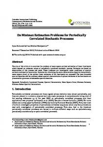
In many real-life networks, the link weights are uncertain because of inaccurate Network State Information (NSI) [11], Equivalently, we could formulate w(li ) ⊕ w(lj ) = ρi,j · [12]. For instance, Papagiannaki et al. [13] showed that the (w(li )+w(lj )), where ρi,j stands for the correlation coefficient queuing delay distribution can be approximated by a Weibull between links li and lj , and its value varies in (0, ∞), since distribution. Since the Cumulative Density Function (CDF) of we do not consider negative costs. When ρi,j is equal to 1, it a Weibull distribution is log-concave and the CDFs of many indicates that li and lj are uncorrelated, when ρi,j is greater common distributions (e.g., Exponential distribution, Uniform than 1, it indicates that li and lj have an increasing correlation, distribution, etc.) are log-concave [14], [15], we make, as in otherwise we say li and lj have a decreasing correlation. [11], [16], a mild (general) assumption that the link l’s weight Analogously, for given m > 1 links l1 , l2 , ..., lm in the follows a log-concave distribution. deterministic correlated model, their joint total cost can be We first define the Correlated Group (CG): expressed as follows: Definition 1: Given is a network G(N , L) where N represents a set of N links and L denotes a set of L links. A w(l1 )⊕w(l2 )···⊕w(lm ) = ρ1,2,...,m ·(w(l1 )+w(l2 )+···+w(lm )) Correlated Group (CG) is a subset of links LCG ⊆ L, and (2.1) ∀l ∈ LCG , ∃l0 ∈ LCG \{l}, such that l and l0 are correlated Similarly, if the link l’s weight is multiplicative (e.g., failure (ρl,l0 6= 1). probability), then by using −log(w(l)) to represent its weight Accordingly, the Maximum Correlated Group (MCG) is devalue, Eq. (2.1) also applies. The decreasing correlation case fined as a CG with the maximum number of correlated links. can also reflect SRLG networks. For instance, in SRLG netIf a link l is uncorrelated/independent with all the other links, works, each link is associated with several SRLG events with then we say {l} is a single element MCG. Suppose there their respective failure occurring probabilities. Hence, the total are Ω Maximum Correlated Groups (MCGs), and there are failure occurring probabilities (represented by PSRLG ) of two i ) in the i-th MCG, where mi > 0 links (denoted as l1i , l2i ,...,lm i correlated links that have at least one SRLG in common will 1 ≤ i ≤ Ω. Each link l has an upper bound of allocating cost be equal to the product of the failure occurring probabilities wlmax . In the i-th MCG, a multivariate mi dimensional logof all the distinct SRLG events that belong to these two links. concave Cumulative Density Function CDFi (x1 , x2 , ..., xmi ) Let us denote Pl1 = Ps1 · Ps and Pl2 = Ps2 · Ps as the i is given to allocate cost x1 , x2 ,..., xmi for links l1i , l2i ,..., lm , i failure probability of these two links, respectively, where Ps respectively. denotes the overlapped SRLGs’ failure occurring probability Therefore, if the possible cost of link l ranges from between l1 and l2 , and Ps1 (Ps2 ) is the non-overlapping 0 to wlmax (0 < wlmax ), then the probability of allocatSRLGs’ failure probability of l1 (l2 ). Then we can have ing a cost value out of this range is 0. Hence, we have Pl1 · Pl2 < PSRLG = Ps1 · Ps2 · Ps < min(Pl1 , Pl2 ). By CDFi (wlmax ) = 1 for a single element MCG i, and taking the −log on this inequality, we have: , wlmax , ..., wlmax ) = 1 for a multi-element MCG CDFj (wlmax j j j mj 1 2 j. max(−log(P1 ), −log(P2 )) < −log(PSRLG ) < (−log(Pl1 )) + (−log(Pl2 )) For example, Fig. 2 shows a 2-dimensional multivariate Or equivalently, Normal distribution, where both variables are in the range −log(PSRLG ) = ρ · (−log(Pl1 )) + (−log(Pl2 )) (2.2) [0, 4] with  mean 2, and the corresponding covariance ma0.9 0.4 trix is . Similarly to Eq. (2.3), the correlation where ρ < 1 denotes their correlation coefficient. 0.4 0.3 Fig. 1: An example of the deterministic correlated model.

matrix (composed of linear correlation coefficients) can be derived from the covariance matrix and the variables’ standard variances in the multivariate Normal distribution. However, we do not explicitly use the linear correlation coefficient in the stochastic correlated model, since we will later prove that via the log-concave property of this model, the shortest path problem under this model can be solved by convex optimization.

CDF(x1,x2)

0.9 1

0.8

0.8

0.7

0.6

0.6 0.5

0.4

0.4

0.2

0.3 0 4

0.2 3

4 3

2

x2

0.1

2

1

1 0

0

x1

Fig. 2: A 2-dimensional multivariate Normal distribution. III. S HORTEST PATH IN C ORRELATED N ETWORKS A. Shortest Path under the Deterministic Correlated Model Definition 2: Given is a directed network G(N , L), and each link l ∈ L has a cost w(l) following the deterministic correlated model. The Shortest Path under the Deterministic Correlated Model (SPDCM) problem is to find a path from the source s to the destination t with minimum cost. In conventional deterministic networks, a subpath of a shortest path is also the shortest. We refer to this property of the shortest path as the dominance of the subpath. However, this is not the case in networks with deterministic correlated link weights, which means a dominated path may also lead to an optimal solution. For instance, in the example of Fig. 1, we can see that although subpath s-b has a smaller cost than subpath s-a-b, path s-a-b-t (instead of path s-b-t) has the minimum cost. In the following, we will study the complexity of the SPDCM problem. Theorem 1: The SPDCM problem is NP-hard. Proof: When the correlation coefficient is equal to 1, the SPDCM problem can be solved by a conventional shortest path algorithm in polynomial time. We therefore prove in the following that the SPDCM problem is NP-hard for “increasing correlation”> 1 as well as “decreasing correlation”< 1. Increasing Correlation: When the correlation coefficient is greater than 1, we make a reduction to the forbidden pairs shortest path problem, which is known to be NP-hard [17]. In a given network and for given set of node pairs ζ, the forbidden pairs shortest path problem looks for the shortest path between s and t such that at most one node from each pair in the set ζ lies on this path. Let us

consider a network with deterministic correlated link weights, where two nodes i and j form a forbidden pair, their costs are correlated such that w(i, .) ⊕ w(j, .) = +∞, where (i, .) and (j, .) represent any link that contains an end node of i and j, respectively. In all the other cases, the link costs are uncorrelated and finite. Since w(i, .) ⊕ w(j, .) = +∞, if the two forbidden nodes appear in the same path then the cost of this path will be +∞, so it will never be the minimum cost path. Now, the SPDCM problem is equivalent to the forbidden pairs shortest path problem. Decreasing Correlation: When the correlation coefficient is less than 1, we make a reduction to the Minimum Color Single-Path (MCSiP) problem, which is NP-hard [18]. Given a network G(N , L), and given the set of colors C = {c1 , c2 , ..., cg } where g is the total number of colors in G, and given the color set {cl } associated to each link l ∈ L, the Minimum Color Single-Path (MCSiP) problem is to find one path from source node s to destination node t such that it uses the least amount of colors. Assume each color ci is associated with cost 1, where 1 ≤ i ≤ z. We further assume that w(l1 )⊕w(l2 )⊕···⊕w(lm ) = x, where x is the total number of distinct colors belonging to these m links. Hence, the SPDCM problem is equivalent to the MCSiP problem. Theorem 2: The SPDCM problem cannot be approximated to arbitrary degree in polynomial time, unless P=NP. Proof: We prove it by contradiction. Increasing Correlation: Assume a polynomial-time approximation algorithm exists that can find a path with a cost at most α · opt, where α > 1 is an approximation ratio. For a pair of forbidden nodes i and j, we further assume w(i, .) ⊕ w(j, .) > α ∗ opt. Therefore, if an approximation algorithm can find a path ψ with cost at most α ∗ opt from s to t, then i and j cannot be simultaneously traversed by this path ψ, which means that the forbidden pairs shortest path problem can be solved in polynomial time, which results in a contradiction. Decreasing Correlation: We first introduce the Disjoint Connecting Path problem [19]. Given a directed network G(N , L), a collection of disjoint node pairs (s1 , t1 ), (s2 , t2 ), ..., (sz , tz ), does G contain z mutually link-disjoint paths, one connecting si and ti for each i, 1 ≤ i ≤ z. This problem is NP-hard when z ≥ 2. Assume a polynomial-time approximation algorithm exists that can find a path with a cost at most α · opt, where α > 1 is an approximation ratio. Assuming all the links in the network have weight 1, and link (u, v) and any m > 0 links in L\{(u, v)} are correlated, with a total cost of β1 · m. Moreover, any two or more links in L\{(u, v)} are assumed to be uncorrelated/independent. According to this assumption, the minimum value of a shortest path is 1 if link (u, v) is not traversed, i.e., it traverses only one link from s to t. However, the optimal solution which traverses link (u, v) has a total cost of opt = β1 · c, where c is the sum of minimum hops from s to u and from v to t. For any given α, let βc > α, then 1 > α · β1 · c, which means

1 > α · opt. To find a path with cost at most α · opt, the polynomial-time algorithm must find a path which traverses link (u, v). In that case the algorithm can, in polynomial time, find two link-disjoint paths from s to u, and from v to t, which results in a contradiction. Next, we study the performance of a conventional shortest path algorithm running on a graph where each link has an “uncorrelated” weight value. Lemma 1: When all the correlation coefficients are greater than 1, a conventional shortest path ψ has a total cost at most ρmax ρopt · opt, where ρmax and ρopt are the largest correlation coefficient and optimal solution’s correlation coefficient, respectively, and opt is the cost P of the optimal solution. Proof: LetPU (ψ) = l∈ψ w(l) and let C(ψ) = ρu · U (ψ) = ρu · l∈ψ w(l) reflect the total joint cost of path ψ considering their correlation, where ρu indicates the correlation coefficient of path ψ. On one hand, a conventional . On the other hand, shortest path ψ should satisfy U (ψ) ≤ ρopt opt C(ψ) ≤ ρmax · U (ψ) considering ρmax is the largest correlation coefficient. Hence, C(ψ) ≤ ρmax · U (ψ) ≤ ρρmax · opt. opt

The pseudo-code of the exact algorithm is given in Algorithm 1.

Lemma 2: When all the correlation coefficients are less than 1 1, a conventional shortest path ψ has a cost at most ρmin · opt, where ρmin is the smallest correlation coefficient among all the correlation coefficients.P l∈ψ w(l) and let C(ψ) = ρu · P Proof: Let V (ψ) = w(l) reflect the total joint cost of path ψ considering l∈ψ their correlation. Since all the correlations are decreasing (ρ < 1), we have C(ψ) ≤ V (ψ). On the other hand, ρmin · V (ψ) ≤ opt considering that ρmin is the smallest correlation coefficient. 1 · opt. Hence, C(ψ) ≤ V (ψ) ≤ ρmin Via Lemmas 1 and 2, we obtain Theorem 3. Theorem 3: In a network with links following the deterministic correlated model, a conventional shortest path can have 1 cost at most max( ρρmax , ρmin ) · opt. opt Theorem 3 reveals that a conventional shortest path may have arbitrary bad performance, since either ρρmax can be opt infinitely large or ρmin can be infinitely small.

C. Shortest Path under the Nodal Deterministic Correlated Model

B. An Exact Algorithm to Solve the SPDCM problem To solve the SPDCM problem exactly, we modify Dijkstra’s algorithm by letting each node store as many subpaths as possible, which is similar to the exact algorithm for solving multi-constrained routing problem [20]. Since each node can store as many subpaths as possible, its running time is exponential. We start with some notations used in the algorithm: sus[u][h]: the parent node of node u for its stored h-th subpath from s to it. dist[u][h]: the cost value stored at node u for its stored h-th subpath from s to it. counter[u]: the number of stored subpaths of node u. u[m]: node u’s stored m-th subpath from s to it. adj(u): the set of adjacent nodes of node u.

Algorithm 1 SP DCM (G, s, t) 1:

2: 3: 4: 5: 6: 7: 8: 9: 10: 11: 12:

Q ← s, P ← ∅, dist[s][1] ← 0, dist[i][h] ← +∞, sus[i][h] ← i, counter[s] ← 1, counter[i] ← 0, ∀i ∈ N \{s}. While Q 6= ∅ u[m] ← Extract-min(Q) If (u == t) do Insert (P , u[m]) Else Foreach v ∈ adj(u) do counter(v) = counter(v) + 1 Calculate the total cost of subpath u[m] → v and assign it to dist[v][counter(v)] sus[v][counter(v)] ← u Insert (Q, v, counter(v)) return min(P ).

In some real-world networks (e.g., SRLG networks), the links that are spatially (geographically) close to each other are usually correlated whereas the links that are located spatially far from each other are usually uncorrelated. We make an additional assumption, which is that only the links sharing the same node can be correlated. We name this kind of correlation as nodal correlation. Although the SPDCM problem is NP-hard, we will show that, by transforming the original graph to an auxiliary graph, the Shortest Path under the Nodal Deterministic Correlated Model (SPNDCM) problem is polynomial-time solvable. For any node a, there are generally two cases of nodal correlation, namely (1) links in the form of (a, b) and (a, c), and (2) links in the form of (a, b) and (b, c) are correlated. When (a, b) and (a, c) are correlated, a simple path cannot traverse both of them since looping is not allowed. In this sense, any simple path only traverses at most one of them, which means that the links’ correlation will not affect the cost calculation of any simple path. Therefore, we only need to consider the case when (a, b) and (b, c) are correlated. We first define that if (a, b) and (b, c) are correlated, then a and b are called correlated nodes, which is represented by Cn , else they are uncorrelated nodes, which is denoted by Un . Subsequently, based on the original graph G(N , L), the auxiliary graph GA (N A , LA ) can be constructed as follows: 1) For any two links (u, v) ∈ L and (v, w) ∈ L that are correlated in G, create new nodes uv , v uw and vw in GA if they do not exist. 2) For any node a ∈ N and if it is an uncorrelated node (in Un ), create node aa in GA . 3) For any two correlated links (u, v) and (v, w) in G, create links (uv , v uw ), (v uw , vw ) and (vw , ww ) in G A .

Assign the links (uv , v uw ) and (vw , wr ) with the weights of w(u, v) and w(v, w), respectively, and the link (v uw , vw ) with the weight of (ρ(u,v)(v,w) −1)·(w(u, v)+ w(v, w)), where ρ(u,v)(v,w) is the correlation coefficient of links (u, v) and (v, w). 4) For each link (a, b) ∈ L such that both node a and node b are not correlated nodes, create the link (aa , bb ) also in GA with the link weight of w(a, b). 5) For each link (a, b) ∈ L such that a ∈ Un and b ∈ Cn , draw links (aa , br ) in GA , where r ∈ N and br ∈ GA . 6) For each link (a, b) ∈ L such that a ∈ Cn and b ∈ Un , draw links (arp , bb ) in GA , where r, p ∈ N and arp ∈ N A.

correlated node to an uncorrelated node in the original graph, e.g., (c, d) in Fig. 3, we draw link (cbt , dd ) to represent it (Step 6). Considering that there are at most N (N − 1) nodal links in a graph, the original graph can be transferred to the auxiliary graph in polynomial time. Consequently, running a shortest path algorithm on the auxiliary graph can return a minimum cost path under the nodal deterministic correlated model. Our auxiliary graph can deal with both decreasing and increasing correlation cases. Considering that (ρ(u,v)(v,w) − 1) · (w(u, v) + w(v, w)) < 0 in the auxiliary graph under the decreasing correlation case, and Dijkstra’s algorithm cannot handle negative link weights, we could for instance run Bellman-Ford’s algorithm on the auxiliary graph. D. Shortest Path under the Stochastic Correlated Model

Fig. 3: An example network with dotted links following the nodal deterministic correlated model.

b

1

ac

(ρ12-1)(w1+w2) c

2

bt

(ρ23-1)(w2+w3) 8

6

1 ad

5

(ρ14-1)(w1+w4) d

4

3

t

t

9 d

6 7 e

Fig. 4: Auxiliary graph of Fig. 3 for the SPDCM problem under the nodal deterministic correlated model. The idea of the auxiliary graph is that if two links (u, v) and (v, w) are correlated, we create four corresponding nodes uv , v uw , vw , ww and then draw three links (uv , v uw ),(v uw , vw ) and (vw , ww ). We use (uv , v uw ) and (vw , ww ) to indicate their uncorrelated value, respectively, if only one of these two links is traversed, and (v uw , vw ) to represent the correlated loss (decreasing correlation)/gain (increasing correlation), respectively, if they are traversed simultaneously. For instance, in Fig. 3 where the link weight is labeled above each link, assuming links (a, b), (b, c), (c, t) and (b, d) are nodal correlated, then Fig. 4 is its corresponding auxiliary graph with the assigned weight shown on each link. In particular, since (a, b), (b, c) and (a, b), (b, d) may have different correlation coefficients, in Fig. 4 we use (bac , bc ) and (bad , bd ) to represent their correlation value, respectively. Meanwhile, when there is a link from an uncorrelated node to a correlated node in the original graph, e.g., (e, b) in Fig. 3, we draw links (ee , bc ) and (ee , bd ) to reflect it (Step 5); When there is a link from a

The Shortest Path under the Stochastic Correlated Model (SPSCM) problem is defined as follows: Definition 3: The Shortest Path under the Stochastic Correlated Model (SPSCM) problem: In a given directed graph G(N , L) where the link costs follow the stochastic correlated model, it is assumed that there are in total Ω Maximum Correlated Groups (MCGs). The SPSCM problem is to find a path from the source s to the destination t such that its total cost is minimized and the probability to realize this value is no less than Ps . We present a convex optimization formulation to solve the SPSCM problem. Convex optimization problems can usually be solved quickly and accurately with convex optimization solvers [21]. Let us first introduce how to develop a Linear Programming (LP) formulation to solve the shortest path problem in deterministic networks: Objective: max dt (3.1) Constraints: ds = 0

(3.2)

dv − du ≤ w(u, v) ∀(u, v) ∈ L

(3.3)

where du is a value between 0 and 1. Similarly, the SPSCM problem can be solved by the following convex formulation: Objective: max dt (3.4) Constraints:

X

ds = 0

(3.5)

dv − du ≤ f (u, v) ∀(u, v) ∈ L

(3.6)


i − log CDFi (f (l1i ), f (l2i ), ..., f (lm )) ≤ − log(Ps ) i

i∈Ω

(3.7)

i ) indicate where the variables f (u, v), f (l1i ), f (l2i ), ..., f (lm i i i i the cost of links (u, v), l1 , l2 ,..., lmi , respectively. Constraint (3.7) ensures that the total probability of realizing the total cost is no more than Ps . In Eq. (3.7), for each MCG we apply the multi-dimensional CDF functions to calculate the probability of realizing a cost. Since the multi-dimensional CDF function is log-concave,
i )) − log CDFi (f (l1i ), f (l2i ), ..., f (lm is convex, and by i summing all the MCGs’ CDFs together, it remains convex, which indicates that Eq. (3.7) is convex. The other constraints are also convex, which proves that the above formulation is a convex optimization model.

E. Widest Path under the Deterministic Correlated Model The Widest Path in Deterministic Networks (WPDN) problem is to find a path from s to t such that the minimum link weight among all its traversed links is maximized. This problem is defined when the link weight is a bottleneck metric such as bandwidth. For example, the bandwidth of a path is equal to minimum link’s bandwidth among all its traversed links. The WPDN problem is polynomial-time solvable: First, we order all the link weights in the network in an increasing order. After that, each round we prune a lowest weight link in the graph and run a Depth First Search (DFS) or a Breadth First Search (BFS) algorithm to find a path from s to t. The algorithm will end if there is no path anymore from s to t and return the pruned weight value of the previous round. In the Widest Path under the Deterministic Correlated Model (WPDCM) problem, if m > 1 correlated links in a path have a joint weight value W , then for each link the maximum average/amortized weight is W m . For instance, if a path traverses three correlated links which have a joint weight value of 15 and passes another uncorrelated link with weight of 6, then this path has a “width” value of 5. The reason is that the maximum (average/amortized) weight for each of these three correlated links is 15/3 = 5, and this value is less than another uncorrelated link’s (6). However, the WPDCM problem is still NP-hard and cannot be approximated to arbitrary degree. The proof follows analogously from Theorems 1 and 2, and therefore we omit it. IV. M IN -C UT IN C ORRELATED N ETWORKS A. Min-Cut under the Deterministic Correlated Model Definition 4: The Min-Cut under the Deterministic Correlated Model (MCDCM) problem: Given is a network G(N , L), and each link l ∈ L is associated with a cost w(l). It is assumed that two or more link costs are correlated under the deterministic correlated model. Given a source s and a target t, to find a cut C which partitions G into two disjoint subsets X (X ∈ N ) and N − X such that s and t are in different subsets and the cost of the cut C is minimized. The min-cut value is not equal to the maximum flow value under the deterministic correlated model. For example, in Fig. 5 assume links (s, a) and (s, t) are correlated with the joint cost of 8. In this example, the maximum flow from s to

c(s,a)  c(s, t )  8 Fig. 5: An example to illustrate that the maximum flow is not equal to the min-cut in correlated networks. t is s − a − t with the maximum flow of 10, while the min-cut which is composed of links (s, a) and (s, t) has cost of 8.

Fig. 6: NP-hardness of the MCDCM problem.

x1 s z1

y3

y2

y1 z2

xn

x3

x2

z3

yn-1

t zn

Fig. 7: A reduction of the MCDCM problem to the SPDCM problem. Theorem 4: The MCDCM problem is NP-hard. Proof: In Fig. 6, we assume that the links in the form of (xi , xi+1 ) and (zi+1 , zi ) have infinite uncorrelated cost and the link costs of (xi , yi ) and (yi , zi ) follow the deterministic correlated model, where 1 ≤ i ≤ n. We want to find a min-cut to separate x1 and z1 . Based on Fig. 6, we first derive Fig. 7 with the same nodes except that we add one more node s. We regard s = y0 , and t = yn . The link weight in Fig. 7 is

set like this: (yi−1 , xi ) and (yi−1 , zi ) have 0 uncorrelated cost, while (xi , yi ) and (zi , yi ) have the same (correlated) costs with (xi , yi ) and (yi , zi ) in Fig. 6, respectively, where 1 ≤ i ≤ n. In Fig. 7, we want to solve the SPDCM problem from the source s to the destination t. Since we want to find a min-cut that separates x1 and z1 , any cut in the form of (xi , yi ) and (yi , zi ), where 1 ≤ i ≤ n, is not the optimal solution. The reason is that this kind of cut only separates yi and other nodes, but not x1 and z1 . Moreover, considering the links in the form of (xj , xj+1 ) or (yj , yj+1 ) have infinite costs, it cannot be in the optimal solution. Based on above analysis, any feasible cut C should contain one link of either (xi , yi ) or (yi , zi ), for all 1 ≤ i ≤ n. We prove in the following that the MCDCM problem in Fig. 6 can be reduced into the SPDCM problem in Fig. 7 in polynomial time. The SPDCM problem to the MCDCM problem: Considering an optimal solution of the SPDCM problem, and denote RSP DCM as the set of links in the optimal solution of the SPDCM problem. Because RSP DCM has minimum cost, let CM CDCM = RSP DCM \{(yi , xi+1 ), (yi , zi+1 )} and then ∀(zi , yi ) ∈ CM CDCM , change it to (yi , zi ) in CM CDCM . Since the links (yi , xi+1 ) and (yi , zi+1 ) have 0 cost, CM CDCM has also minimum cost (the same with RSP DCM ). Therefore solving the SPDCM problem yields a solution to the MCDCM problem. The MCDCM problem to the SPDCM problem: An optimal solution of the MCDCM problem should be composed of either (xi , yi ) or (yi , zi ), where 1 ≤ i ≤ n. Denote CM CDCM as the set of links in the optimal solution of the MCDCM problem. Let RSP DCM = CM CDCM and then ∀(yi , zi ) ∈ RSP DCM , change it to (zi , yi ) in RSP DCM . Because CM CDCM has minimum cost value and the links in the form of (yi−1 , xi ) or (yi−1 , zi ) have 0 cost, RSP DCM together with (yi−1 , xi ) if (xi , yi ) ∈ RSP DCM or (yi−1 , zi ) if (zi , yi ) ∈ RSP DCM , can form a path from s to t with minimum cost. Hence, a solution to the MCDCM problem can also solve the SPDCM problem. Theorem 5: The MCDCM problem cannot be approximated to arbitrary degree in polynomial time, unless P=NP. Proof: The proof follows from the fact that the SPDCM problem cannot be approximated to arbitrary degree in polynomial time according to Theorem 2. Theorem 6: By assigning each link l with the cost w(l), running a conventional min-cut algorithm will return a cut 1 with total cost at most max( ρρmax , ρmin ) · opt. opt Proof: The proof follows analogously from Theorem 3, and we therefore have omitted it. Since the MCDCM problem is NP-hard and even does not admit a polynomial-time approximation algorithm, we propose a brute-force algorithm with exponential running time to solve it exactly. The idea is that we start with two sets A and B, with s in A and t in B without loss of
generality. have
Then we
N −2 N −2 nodes left, and there are N 0−2 + N 1−2 +···+ N −2 = O(2N ) combinations to assign these N − 2 nodes to sets A and B. For each combination assignment, it corresponds to a cut to separate A and B, and we calculate the total cost value

of the links which connect both A and B as the cut value. At last, we select one cut with minimum cost as the optimal solution. B. Min-Cut under the SRLG-like Correlated Model In Section II, we introduce and formulate the joint failure calculation in SRLG networks, which follows the decreasing correlated case. We define the SRLG-like correlated model as follows: Definition 5: The SRLG-like correlated model: Suppose l1 , l2 ,...,lm (1 < m ≤ L) form a Correlated Group (CG), then w(l1 )⊕w(l2 )···⊕w(lj ) is greater than the sum of any no more than j −1 links’ cost, but smaller than w(l1 )+w(l2 )···+c(lj ), where 1 < j ≤ m. Unfortunately, the Min-Cut under the SRLG-like correlated model problem is still NP-hard, since it can be reduced to the MCSiP problem via Figs. 6 and 7. In the Nodal SRLG-like correlated model, it is assumed that only the links that share the same node follow the SRLG-like correlated model. As section III-C shows that the Shortest Path under the Nodal Deterministic Correlation Model problem is polynomial-time solvable, we address the Min-Cut under the Nodal SRLG-like correlated model (MC-NSRLG) problem in the following. In general, the MC-NSRLG problem is still NPhard. The reason is that the MC-NSRLG problem in Fig. 8, where the links in the form of (x1 , yi ) are assumed to be correlated, can be reduced to the SPDCM problem in Fig. 7, where the links in the form of (xi , yi ) are assumed correlated (the same with (x1 , yi ) in Fig. 8) and the other links are assumed to have uncorrelated 0 cost.

Fig. 8: NP-hardness of the MC-NSRLG problem. However, we found that the MC-NSRLG problem is polynomial-time solvable when (1) only the nodal links in the form of (u, v) and (v, w) follow the SRLG-like correlated model and/or (2) for any node u ∈ N , at most two nodal links (u, v) and (u, x) follow the SRLG-like correlated model. To prove case (1), let us first study the following theorem:

Theorem 7: Any two links in the form of (u, v) and (v, w) will never both appear in the optimal solution of the MCNSRLG problem in case (1). Proof: Suppose s and t are separated by a min-cut C such that s is in the subset A and t is in the subset B. We prove it by contradiction and thus we assume (u, v) and (v, w) are both in the min-cut C. Since C is the min-cut which separates s and t, then node u should be in subset A, otherwise if node u is in the subset B, there is no need to use (u, v) and (v, w) as the cut links since their existence does not affect the connectedness between A and B. In this sense, node v is in the subset B, otherwise if node v is also in A, there is no need to cut link (u, v). Based on this analysis, if w is in A, then (v, w) is not necessarily the link in the cut C, since link (v, w) does not affect the connectedness from A to B. This results in a contradiction; If node w is in B, link (v, w) is also not necessarily the link in the optimal min-cut, since nodes v and w are in the same subsets, which results in a contradiction. Based on Theorem 7, we can use conventional Linear Programming (LP) for solving the min-cut problem in deterministic networks to solve the MC-NSRLG problem under case (1). According to [22], the LP is as follows. Objective: X min c(u, v) · hu,v (4.1)

represent the total cost of links (v, u) and (x, u), where ρvx represents the correlation coefficients between (v, u) and (x, u). 4) For any link (a, u) ∈ L\{v, x} and (u, b) ∈ L such that (v, u) and (x, u) are correlated in G, draw link (a, u0 ) and (u0 , b) in GU with the weight of w(a, u) and w(u, b), respectively. 5) For the other links (c, d) ∈ L in G except for above four cases, create link (c, d) also in GU with the same weight. The proposed auxiliary graph here shares similarities with the auxiliary graph in Fig. 4. As an example, Fig. 10 is an auxiliary graph of the original graph shown in Fig. 9. Moreover, we mention that the proposed auxiliary graph also applies when there are m > 2 links starting from the same node that follow the SRLG-like correlated model, but as long as one correlated link “encounters failure”, the other m−1 links simultaneously “fail” (e.g., SRLG networks, inter-dependent networks).

W5

W2 W1

W3

(u,v)∈L0

W6

W4

W8

W7

Constraints: hs,t ≥ 1

hu,v + hv,w ≥ hu,w , ∀u, v, w ∈ N : u 6= v 6= w

(4.2)

Fig. 9: An example network with dotted links following the SRLG-like correlated model.

(4.3) W2

hu,v ≥ 0, ∀u, v ∈ N : u 6= v

(4.4)

where c(u, v) stands for the link weight (i.e., capacity) of link (u, v) in the deterministic network and hu,v is an indicator denoting whether (u, v) belongs to the cut. Under case (2), the MC-NSRLG problem can be solved by running the above LP (Eqs. (4.1)-(4.4)) on an auxiliary graph GU (N U , LU ) in polynomial time. The auxiliary graph can be derived from the original graph G as follows: 1) For each pair of two links (u, v) ∈ L and (u, x) ∈ L that are correlated in G, create a new node u0 , and draw link (u0 , u) with the weight of ρvx (w(u, v)+w(u, x)) to represent the joint cost of links (u, v) and (u, x), where ρvx represents the correlation coefficients between (u, v) and (u, x). 2) For any link (a, u) ∈ L and (u, b) ∈ L\{v, x} such that (u, v) and (u, x) are correlated in G, draw link (a, u0 ) and (u0 , b) in GU with the weight of w(a, u) and w(u, b), respectively. 3) For each pair of two links (v, u) ∈ L and (x, u) ∈ L that are correlated in G, create a new node u0 , and draw link (u, u0 ) with the weight of ρvx (w(v, u)+w(x, u)) to

W1

W5 W3

ρ56(w5+w6)

W6

W8

ρ34(w3+w4) W4

W7

Fig. 10: Auxiliary graph of Fig. 9 for the MC-NSRLG problem.

C. Min-Cut under the Stochastic Correlated Model The Min-Cut under Stochastic Correlated Model problem can be defined as follows: Definition 6: The Min-Cut under Stochastic Correlated Model (MCSCM) problem: In a given directed graph G(N , L) with link costs following the stochastic correlated model, the MCSCM problem is defined to find a cut C which partition G into two disjoint subsets X (X ∈ N ) and N − X such that: • s and t are in different subsets. • the allocated cost of the cut C is minimum. • the total probability of realizing the cost value is no less than Pc .

We propose a convex optimization formulation to solve it. Based on Eq. (4.1)-Eq. (4.4), the MCDCM problem under the correlated stochastic model can be solved by the following convex optimization formulation: Objective: X min f (u, v) · hu,v (4.5) (u,v)∈L

Constraints: X


i )) ≤ − log(Pc ) − log CDFi (f (l1i ), f (l2i ), ..., f (lm i

i∈Ω

(4.6) 0 ≤ f (u, v) ≤ cmax (u,v) ∀(u, v) ∈ L

(4.7)

hs,t ≥ 1

(4.8)

hu,v + hv,w ≥ hu,w , ∀u, v, w ∈ N : u 6= v 6= w hu,v ≥ 0, ∀u, v ∈ N : u 6= v

(4.9) (4.10)

i ) indicate the allocated where f (u, v), f (l1i ), f (l2i ), ..., f (lm i i i , respectively. In possible cost by links (u, v), l1 , l2i ,..., lm i particular, Eq. (4.6) ensures that the probability of realizing the sum of allocated cost of the min-cut is no less than Pc . More specifically, for each MCG we apply the multi-dimensional CDF functions to calculate the probability of realizing possible cost. Since the CDF function
is logi )) is conconcave, then − log CDFi (f (l1i ), f (l2i ), ..., f (lm i vex, by summing all the MCGs together, it remains convex, which indicates that Eq. (4.6) is convex. It remains to show that Eq. (4.5) is convex. In general, the product of two convex functions is not always convex, however, according to [21, pp. 119], one special case is: “If functions f and g are convex, both nondecreasing (or nonincreasing), and positive (nonnegative) functions on an interval, then f · g is convex.” Therefore, for each (u, v) ∈ L, f (u, v) · hu,v is convex.

V. R ELATED W ORK A. Routing with correlated link weights In a network with each link having multiple additive link weight metrics (e.g., delay, cost, jitter, etc.), the Quality of Service (QoS) routing problem is to find a path that satisfies a given metric vector constraint. Kuipers and Van Mieghem [23] study the QoS routing problem under uncorrelated link weights. Another common source of correlation is SharedRisk Link Groups (SRLGs). Sometimes one SRLG can also be represented by one color, but they share the same meaning in terms of reliability. In this context, Yuan et al. [18] prove that the Minimum Color Single-Path (MCSiP) problem is NPhard. Yuan et al. also prove that finding two link-disjoint paths with total minimum distinct amount of colors or least amount

of coupled/overlapped colors is NP-hard. Lee et al. [24] propose a probabilistic SRLG framework to model correlated link failures and develop an Integer Nonlinear Programming Programming (INLP) to find one unprotected path or two linkdisjoint paths with the lowest failure probability. There is also some literature dealing with correlated routing problems in stochastic networks [25]. For example, in [26], only two possible states are assumed, which are congested and uncongested, and each state corresponds to a cost value. u,v,w A probability matrix Pa,b , which represents the probability that if (u, v) is in state a then (v, w) is in state b, is given. Two similar link weight models called link-based congestion model and node-based congestion model are proposed in [27]. Based on these models, [26], [27] define and solve the least expected routing problem, which is to find a path from the source to the destination with the minimum expected costs. However, in [26], [27] there are only two possible states for each link and only the correlation of the adjacent links is known/assumed. We assume a more general (and different) stochastic correlated model, where as long as the links (not necessarily adjacent) are correlated, their joint CDF for allocating costs is known. B. Min-Cut in Conventional Networks The (s, t) Min-Cut problem refers to partition the network into two disjoint subsets such that nodes s and t are in different subsets and the total weight of the cut links are minimized. This problem can be solved by finding the maximum flow from s to t according to [28]. There is also a lot of work on the Min-Cut problem with no specified node pairs (s, t). A summary and comparison of the existing classical polynomialtime algorithms to solve the Min-Cut problem can be found in [29]. The fastest algorithm to solve the Min-Cut problem which has a time complexity of O(L log3 N ) is proposed by Karger [30]. Accordingly, the Min-Cut problem can be tackled by solving at most N − 1 times of the (s, t) Min-Cut problem. C. Constrained Maximum Flow As a dual of the min-cut problem, the maximum flow problem in conventional networks is polynomial-time solvable [28]. However, this problem becomes NP-hard if some constraints are imposed on the links. Suppose that the negative disjunctive constraints indicate that a certain set of links cannot be used simultaneously for the optimal solution, while the positive disjunctive constraints force at least one of a certain set of links to be present in the optimal solution. Pferschy and Schauer [31] prove that the maximum flow problem in both negative and positive disjunctive constraints are NP-hard and do not admit a Polynomial-Time Approximation Scheme (PTAS). Here, the disjunctive constraint corresponds to the correlated link weights in this paper, so the maximum flow problem in correlated networks is also NP-hard and does not admit a PTAS. Assuming the link’s bandwidth and delay follow a log-concave distribution, Kuipers et al. [16] propose a polynomial-time convex optimization formulation to find the maximum flow in the so-called stochastic networks. When the delay constraint is imposed on each path, the maximum flow

problem is NP-hard. To solve it, Kuipers et al. [16] propose an approximation algorithm and a tunable heuristic algorithm. VI. C ONCLUSION In this paper, we have studied the shortest path problem and the min-cut problem in correlated networks under two link-weight models, namely (i) the deterministic correlated model and (ii) the (log-concave) stochastic correlated model. We have proved that these two problems are NP-hard under the deterministic correlated model, and cannot be approximated to arbitrary degree, unless P=NP. Subsequently, we have proposed exact algorithms to solve them. In particular, we have shown that both of them are polynomial-time solvable under a (constrained) nodal deterministic correlated model. For the stochastic correlated model, we have shown that these two problems can be solved by convex optimization. R EFERENCES [1] W. Cui, I. Stoica, and R. H. Katz, “Backup path allocation based on a correlated link failure probability model in overlay networks,” in Proc. of IEEE ICNP, 2002, pp. 236–245. [2] F. A. Kuipers and F. Dijkstra, “Path selection in multi-layer networks,” Computer Communications, vol. 32, no. 1, pp. 78–85, Jan. 2009. [3] S. Savage, A. Collins, E. Hoffman, J. Snell, and T. Anderson, “The endto-end effects of internet path selection,” in ACM SIGCOMM Computer Communication Review, vol. 29, no. 4. ACM, 1999, pp. 289–299. [4] D. Kosti´c, A. Rodriguez, J. Albrecht, and A. Vahdat, “Bullet: High bandwidth data dissemination using an overlay mesh,” in ACM SIGOPS Operating Systems Review, vol. 37, no. 5, 2003, pp. 282–297. [5] K. Kim and N. Venkatasubramanian, “Assessing the impact of geographically correlated failures on overlay-based data dissemination,” in Proc. of IEEE GLOBECOM, 2010, pp. 1–5. [6] S. Trajanovski, F. A. Kuipers, A. Ili´c, J. Crowcroft, and P. Van Mieghem, “Finding critical regions and region-disjoint paths in a network,” IEEE/ACM Transactions on Networking, vol. 23, no. 3, 2015. [7] F. Kuipers, A. Beshir, A. Orda, and P. Van Mieghem, “Impairmentaware path selection and regenerator placement in translucent optical networks,” in Proc. of IEEE ICNP, 2010. [8] S. V. Buldyrev, R. Parshani, G. Paul, H. E. Stanley, and S. Havlin, “Catastrophic cascade of failures in interdependent networks,” Nature, vol. 464, no. 7291, pp. 1025–1028, Apr. 2010. [9] J. Strand, A. L. Chiu, and R. Tkach, “Issues for routing in the optical layer,” IEEE Communications Magazine, vol. 39, pp. 81–87, 2001. [10] G. Dantzig and D. R. Fulkerson, “On the max flow min cut theorem of networks,” Linear inequalities and related systems, vol. 38, pp. 225–231, 2003. [11] D. H. Lorenz and A. Orda, “Qos routing in networks with uncertain parameters,” IEEE/ACM Transactions on Networking, vol. 6, no. 6, pp. 768–778, 1998. [12] R. A. Gu´erin and A. Orda, “Qos routing in networks with inaccurate information: theory and algorithms,” IEEE/ACM Transactions on Networking, vol. 7, no. 3, pp. 350–364, 1999. [13] K. Papagiannaki, S. Moon, C. Fraleigh, P. Thiran, F. Tobagi, and C. Diot, “Analysis of measured single-hop delay from an operational backbone network,” in Proc. of IEEE INFOCOM, vol. 2, 2002, pp. 535–544. [14] M. Bagnoli and T. Bergstrom, “Log-concave probability and its applications,” Economic Theory, vol. 26, no. 2, pp. 445–469, 2005. [15] G. R. Mohtashami Borzadaran and H. A. Mohtashami Borzadaran, “log-concavity property for some well-known distributions,” Surveys in Mathematics and its Applications, vol. 6, pp. 203–219, December 2011. [16] F. A. Kuipers, S. Yang, S. Trajanovski, and A. Orda, “Constrained maxmum flow in stochastic networks,” in Proc. of IEEE ICNP, North Carolina, USA, October 2014. [17] H. Gabow, S. N. Maheshwari, and L. Osterweil, “On two problems in the generation of program test paths,” IEEE Transactions on Software Engineering, vol. SE-2, no. 3, pp. 227–231, 1976. [18] S. Yuan, S. Varma, and J. Jue, “Minimum-color path problems for reliability in mesh networks,” in Proc. of IEEE INFOCOM, vol. 4, 2005, pp. 2658–2669.

[19] M. R. Garey and D. S. Johnson, Computers and Intractability: A Guide to the Theory of NP-Completeness. New York, NY, USA: W. H. Freeman & Co., 1979. [20] P. Van Mieghem and F. Kuipers, “Concepts of exact quality of service algorithms,” IEEE/ACM Transactions on Networking, vol. 12, no. 5, pp. 851–864, 2004. [21] S. Boyd and L. Vandenberghe, Convex Optimization. New York, NY, USA: Cambridge University Press, 2004. [22] A. Tamir, “Polynomial formulations of min-cut problems,” Manuscript, Department of Statistic and Operations Research, Tel Aviv University, Israel, 1994. [23] F. A. Kuipers and P. Van Mieghem, “The impact of correlated link weights on qos routing,” in Proc. of IEEE INFOCOM, vol. 2, 2003, pp. 1425–1434. [24] H.-W. Lee, E. Modiano, and K. Lee, “Diverse routing in networks with probabilistic failures,” IEEE/ACM Transactions on Networking, vol. 18, no. 6, pp. 1895–1907, 2010. [25] S. Yang and F. A. Kuipers, “Traffic uncertainty models in network planning,” IEEE Communications Magazine, vol. 52, no. 2, pp. 172 – 177, 2014. [26] S. T. Waller and A. K. Ziliaskopoulos, “On the online shortest path problem with limited arc cost dependencies,” Networks, vol. 40, no. 4, pp. 216–227, 2002. [27] Y. Fan, R. Kalaba, and J. Moore, “Shortest paths in stochastic networks with correlated link costs,” Computers & Mathematics with Applications, vol. 49, no. 9, pp. 1549–1564, 2005. [28] L. R. Ford and D. R. Fulkerson, “Maximal flow through a network,” Canadian Journal of Mathematics, vol. 8, no. 3, pp. 399–404, 1956. [29] C. S. Chekuri, A. V. Goldberg, D. R. Karger, M. S. Levine, and C. Stein, “Experimental study of minimum cut algorithms,” in Proceedings of the eighth annual ACM-SIAM symposium on Discrete algorithms. Society for Industrial and Applied Mathematics, 1997, pp. 324–333. [30] D. R. Karger, “Minimum cuts in near-linear time,” Journal of the ACM (JACM), vol. 47, no. 1, pp. 46–76, 2000. [31] U. Pferschy and J. Schauer, “The maximum flow problem with disjunctive constraints,” Journal of Combinatorial Optimization, vol. 26, no. 1, pp. 109–119, 2013.