Apr 27, 2012 - spin-glass transition in a random external magnetic field to probe the existence of a ..... required data structures, the minimization of memory accesses, the adherence to the ... the hard drive initial configurations of spins s, interactions J and external magnetic .... to restore a non-tiled layout in shared memory.
EPJ manuscript No. (will be inserted by the editor)
Optimized GPU simulation of continuous-spin glass models
arXiv:1204.6192v1 [physics.comp-ph] 27 Apr 2012
Taras Yavors’kii1 and Martin Weigel1,2 1
2
Institut f¨ ur Physik, Johannes Gutenberg-Universit¨ at Mainz, Staudinger Weg 7, D-55099 Mainz, Germany Applied Mathematics Research Centre, Coventry University, Coventry, CV1 5FB, United Kingdom
Abstract. We develop a highly optimized code for simulating the Edwards-Anderson Heisenberg model on graphics processing units (GPUs). Using a number of computational tricks such as tiling, data compression and appropriate memory layouts, the simulation code combining overrelaxation, heat bath and parallel tempering moves achieves a peak performance of 0.29 ns per spin update on realistic system sizes, corresponding to a more than 150 fold speed-up over a serial CPU reference implementation. The optimized implementation is used to study the spin-glass transition in a random external magnetic field to probe the existence of a de Almeida-Thouless line in the model, for which we give benchmark results.
1 Introduction In spite of a rather substantial concerted research effort extending over more than three decades, a comprehensive understanding of the theory of the spin-glass state is still not within reach. Nevertheless, substantial progress has been made since the suggestion of the Edwards-Anderson Hamiltonian as the standard simplified model of a spin glass in the 1970s [1] and the subsequent formulation of its highly unusual mean-field theory based on the concept of replica-symmetry breaking (RSB) [2]. This concerns, in particular, the nature of the spin-glass phase itself, for which a number of alternative descriptions have been proposed. These include a putative continuation of the RSB theory known to be exact in the mean-field limit to finite-dimensional systems [3] as well as a more conventional picture describing the physics at low temperatures in terms of droplet excitations similar to those found in ferromagnets [4, 5]. In reaction to the conflicting evidence from numerical calculations, more recently several mixed or intermediate scenarios have been suggested as well [6–8]. Still, unequivocal (numerical or analytical) evidence for any of these scenarios could so far not be produced. Another, possibly even more fundamental, issue regards the question of the existence of a spin-glass phase transition for specific spin symmetries and spatial dimensions and, in particular, the determination of the lower critical dimension dl of the spin-glass transition. It has been rather clear since a number of years that the Edwards-Anderson Ising model undergoes a spin-glass transition in three dimen-
2
Will be inserted by the editor
sions [9, 10], but there is no spin-glass phase at non-zero temperatures in two dimensions [11], such that 2 ≤ dl < 3. On the other hand, it is only recently that a consensus emerges as to the lower critical dimension for vector spin glasses. A number of largescale studies has consistently shown the occurrence of a spin-glass transition at finite, but rather low temperatures for the XY [12] and Heisenberg spin glasses [13–16] in three dimensions. Less agreement has been achieved as to the question of the influence of the symmetry group O(n), n > 1, on the ordering of these continuous-spin systems. Following initial suggestions by Villain [17] about the possibility of a decoupling of the Ising like degrees of freedom embedded according to O(n) = SO(n) ⊕ Zn in the order parameter, there is an ongoing debate as to whether two consecutive transitions, corresponding to an ordering of chiral and spin degrees of freedom, can be observed in these systems [12–16, 18]. In the absence of clear-cut field-theoretic and other perturbative approaches for these systems in the relevant regime d < du = 6, much of the progress in the field has relied on the development of new computational techniques and the use of cuttingedge computing hardware for performing extensive computer simulation studies. On the algorithmic side, these included the deployment of the replica exchange or parallel tempering technique [19, 20] as well as, for continuous-spin glasses, the adaptation of the over-relaxation move [14] from its original use in lattice field theory. Besides using the most powerful supercomputers available at each time, the hardware side of this simulational attack to the problem has repeatedly seen the design and construction of special-purpose machines, specifically optimized for the type of simulations at hand. The most recent such enterprise has been the JANUS machine, a special-purpose computer for the simulation of discrete spin systems (mostly used for spin glasses) based on field-programmable gate arrays (FPGA) [21] (see also the review article of the JANUS collaboration in this issue). While such machines are highly efficient, the effort for their design and construction is significant. As an alternative route, one might hence think of using less exotic components that nevertheless provide a massively parallel computing environment. Such hardware is given by current-generation graphics processing units (GPUs). In a number of previous studies, we have investigated the suitability of such devices for the general purpose of simulating lattice spin models [22–25]. One of the observations gleaned from this experience is that within this class of applications a near ideal application for such devices is (a) the study of disordered system due to the inherent trivial parallelism over disorder realizations and (b) systems with continuous spins, since these allow to harvest the large floating-point performance and the benefits of special-function implementations in hardware. The purpose of the present study is to see whether the 3D Heisenberg spin-glass model lives up to its name in this respect and a GPU simulation can be performed with outstanding efficiency.
2 Model and method We consider the nearest-neighbor Edwards-Anderson spin glass model in an external, random magnetic field, X X H=− Jij si · sj − Hi · si . (1) i,j
i
Here, the indices i and j enumerate the sites of a simple (hyper-)cubic lattice of edge length L and the si are m-component classical vectors of unit length. For the purpose of the present paper, we assume m = 3, i.e., Heisenberg spins and d = 3 space dimensions, but it should be clear that our code can be adapted to more general situations
Will be inserted by the editor
3
with rather modest modifications. One exception to this rule is the heat-bath update discussed below, which cannot be formulated in closed form for arbitrary numbers m of spin components. To avoid this problem, however, alternative techniques such as the fast linear algorithm of Ref. [26] can be adapted instead. We further assume nearest-neighbor interactions, which will be important from the algorithmic point-ofview for the efficient use of the massive parallelism available from GPUs using domain decompositions. The nearest-neighbor couplings Jij are quenched, precomputed random variables drawn from a Gaussian distribution with zero mean and standard deviation unity: Jij ∼ N (0, 1) (generalizations to other nearest-neighbor Jij amounts to their precomputation according to a different distribution). Likewise, the on-site magnetic fields Hi are drawn independently from a uniform distribution on an m dimensional sphere of fixed radius |H|. This choice is motivated by the recent work [27] suggesting that considering fields with a random direction (in addition to possibly having a random magnitude) will exhibit a de Almeida–Thouless line (at least) in the mean-field limit of such models, which is in contrast to the findings for vector-spin systems in a uniform field that, instead, exhibit a Gabay–Tolouse line with spin-glass ordering only in the transverse components. We study these systems with a combination of algorithms that is currently considered the best tool-set for the simulation of (continuous) spin glasses (see, e.g., Refs. [14–16]). Importance sampling is performed using heat-bath updates, as these avoid the extra tunable parameter in form of a spin-reorientation amplitude required for Metropolis updates of continuous spins and they are also more efficient in terms of reduced autocorrelation times [26]. The update generates a new spin state s0 on site i independently of the old state s according to the conditional Gibbs distribution for this spin subject to all other spins in the system fixed: s0 ∼ CeβHeff ·s ,
(2)
where β is the inverse temperature, C is a normalization constant and Heff = P 0 J s ij j + H is the local molecular field. The Cartesian components of s can be j explicitly obtained from two random numbers distributed uniformly between 0 and 1, see, e.g., the discussion in Ref. [15]. It has been shown in Ref. [14] that an additional precession of the spins around their local, instantaneous molecular fields can help to significantly speed up the decorrelation in the system. These over-relaxation moves are microcanonical, i.e., they preserve the total energy, and can be implemented very efficiently as they do not involve random numbers [28]. The most efficient implementation and, arguably, the most efficient decorrelation of the states is achieved by simply reflecting each spin at its local molecular field, s0 = 2
s · Heff Heff − s. 2 Heff
(3)
The ratio of the number of over-relaxation to heat-bath updates is an optimization parameter to be tuned to reach the maximal decorrelation effect per clock cycle. As spin-glass systems suffer from notoriously slow dynamics at low temperatures, the equilibrium of these models can hardly be studied for more than the smallest system sizes without further, generalized-ensemble techniques for coping with their complex free-energy landscapes. One efficient approach, that we chose to employ here, is the parallel tempering or replica exchange method [19,20]. There, for every choice of Jij a number RT of copies of system (1) are simulated at a set of different, but close neighboring temperatures Ti . After each copy undergoes a number of local spin updates, for instance the combination of heat bath and over-relaxation moves discussed above, a sweep of attempts to swap pairs i and i + 1 of neighboring configurations with energies Ei and Ei+1 at temperatures Ti and Ti+1 starting from the lowest temperature
4
Will be inserted by the editor
T1 is made, and each swap is accepted according to the Metropolis criterion � � pacc (i ↔ i + 1) = min 1, e∆β∆E .
(4)
Here, ∆E = Ei+1 − Ei and ∆β = 1/Ti+1 − 1/Ti . With an appropriate choice of temperatures, this update allows for configurations with slow dynamics at low temperatures to successively diffuse to high temperatures, decorrelate there and return back to the low-temperature phase, likely arriving in a different valley of a complex free-energy landscape. The choice of temperatures as well as the local frequency of swap attempts can be optimized to ensure an optimal decorrelation effect [29–31]. To study spin-glass phase transitions undergone by such systems, due to the severely restricted system sizes one is able to equilibrate, some effort needs to be invested in devising well-suited finite-size scaling analyses. One of the most successful approaches for spin glasses and other disordered systems [32] concentrates on the role of the finite-size spin-glass correlation length ξL . This is determined from the Edwards-Anderson order parameter, q µν =
1 X µ(1) ν(2) s si , N i i
(5)
where µ, ν are spin components and “(1)” and “(2)” denote two copies of model (1) with identical interactions which are simulated in parallel. We first consider the case of a vanishing external magnetic field and define the wave-vector dependent overlap as 1 X µ(1) ν(2) ik·Ri s si e . (6) q µν (k) = N i i This leads to the k-dependent spin glass susceptibility χSG (k) = N
X
2
[h|q µν (k)| i]J ,
(7)
µ,ν
where h· · · i denotes a thermal average and [· · · ]J denotes an average over disorder. The standard second-moment definition of the correlation length is then given by ξL =
1 2 sin(kmin /2)
�
χSG (0) −1 χSG (kmin )
�1/2 (8)
with kmin = (2π/L)(1, 0, 0). To allow for a more detailed analysis of χSG (k) [33] we record a small number of additional modes. For the case of non-vanishing magnetic fields Hi , one needs to subtract the disconnected part of the spin-glass correlation function such that [34] χSG (k) =
1 X X µν 2 ik·(Ri −Rj ) [(χ ) e ]J , N i,j µ,ν ij
(9)
where µ ν µ ν χµν ij = hsi sj i − hsi ihsj i. 2 In practice, we estimate (χµν ij ) by simulating in parallel four distinct real replicas with the same disorder configuration, using samples from the time series to compute
Will be inserted by the editor
5
the averages X X µ(1) ν(1) µ(2) ν(2) χ1 (k) = h si sj si sj eik·(Ri −Rj ) i, i,j µ,ν
X X µ(1) ν(1) µ(3) ν(4) χ2 (k) = h si sj si sj eik·(Ri −Rj ) i,
(10)
i,j µ,ν
X X µ(1) ν(2) µ(3) ν(4) χ3 (k) = h si sj si sj eik·(Ri −Rj ) i, i,j µ,ν
and assembling them at the end of the simulation to yield χSG (k) =
1 [χ1 (k) − 2χ2 (k) + χ3 (k)]J . N
(11)
The correlation length itself is calculated from the same Eq. (8) as for the zero-field case. In contrast to ferromagnets, where the symmetry group of the order parameter is S n , the n-dimensional unit sphere, the lack of long-range order in spin glasses results in a symmetry group of O(n), including proper as well as improper rotations. Correlations in the embedded reflection degrees of freedom, or chiralities, are not directly captured by the (spin) correlation length (8). To examine the possibility of a decoupling of spin and chiral degrees of freedom, we therefore additionally consider the chiral correlation length which is sensitive to such correlations. Following Ref. [35], we define the local chirality in terms of three spins on a line as κα ˆ · si × si−α ˆ. i = si+α
(12)
Here, α ˆ denotes one of the basis vectors of the lattice’s unit cell. In analogy to the spin degrees of freedom, we then define the chiral overlap, 1 X α(1) α(2) ik·Ri qcα (k) = κ κi e , (13) N i i and the corresponding, wave-vector dependent chiral susceptibility for zero magnetic field, 2 α χα (14) CG (k) = N [h|qc (k)| i]. This, finally, allows us to define the chiral correlation length as �1/2 � α χCG (0) 1 α −1 . ξc,L = 2 sin(kmin /2) χα CG (kmin )
(15)
To the extent it is affected by external fields, the chiral correlation length for the case of non-vanishing fields can be estimated from four-replica expressions analogous to Eq. (10). In addition, we consider some more fundamental quantities such as the 2 internal energy UL (T ) = [hHi] and specific heat CL (T ) = 1/T 2 [hH2 i − hHi ]. Further observables, for instance the spin-glass Binder cumulants, can also easily be measured additionally with only small computational overhead, but we will not discuss them here.
3 Implementation The locality of interactions, the natural prevalence of relatively expensive floatingpoint operations such as those required for the heat-bath update, and the large number of fully or nearly independent systems introduced by the required average over
6
Will be inserted by the editor
disorder realizations and the parallel-tempering update, make the present problem near ideally suited for simulations on the massively parallel architecture provided by current GPU devices. Building on our previous experience with simulating spin models on GPU [23, 25], we here concentrate on a CUDA implementation for NVIDIA devices, although a more general OpenCL realization would be feasible along rather similar lines. While parallelization over (nearly) independent system replicas is almost trivial to achieve algorithmically, the performance on GPU devices is, at least for the problem at hand, strongly dominated by the efficiency of memory accesses. Hence, significant effort needs to be devoted to the optimal memory layout of the required data structures, the minimization of memory accesses, the adherence to the preferred memory access patterns of the GPU devices (coalescence and avoidance of bank conflicts), and the efficient use of the intrinsic memory hierarchy of global memory, shared memory and registers. Technical details about these issues can be found, for instance, in Refs. [36, 37]. Naturally, the completely independent simulations of different disorder realizations are easily parallelized also over different GPU devices, which we indeed use in practice. For simplicity, however, we confine our discussion in the present article to the description of a single-GPU code.
3.1 Double checkerboard decomposition The locality of interactions and spin updates allows us to use a straightforward domain decomposition. For a bipartite lattice, such as the cubic lattice of model (1), the natural way of achieving this is through a (generalized) checkerboard decomposition: all spins on one of two sub-lattices (referred to, for instance, as “even” and “odd”) can be updated in parallel without any need for inter-thread communication. This is illustrated schematically in the left panel of Fig. 1. To make efficient use of the aforementioned memory hierarchy of GPU devices and, in particular, the availability of a small amount (currently up to 48 kB) of shared memory with access latencies around 100 times less than those for accessing global memory, this updating scheme is combined with a caching technique applied to tiles which we have dubbed a double checkerboard decomposition [22, 25]. There, the spin configuration of one of B d tiles (plus a boundary layer) is loaded collaboratively into shared memory and assigned for updating to a thread block. The threads of the block then update the even tile spins in parallel, followed by an update of the odd spins. If these tiles are, in turn, arranged in a checkerboard fashion (leading to the second checkerboard level), updating of tiles of one of two sub-lattices of tiles can occur in parallel without any communication overheads. While the use of shared memory leads to a performance improvement as compared to any non-tiled code for a single system, the tiling turns out to be most beneficial if several updates are performed on each tile before proceeding to loading the next tile [25]. For the present model, we perform several rounds of over-relaxation and heat-bath updates for each tile to ensure an optimal amortization of the tile load overhead.
3.2 General code arrangement We first give a general outline of the code and the compute kernels involved before moving on to discussing some of the used optimizations in more detail in the following section. From a very abstract point-of-view, our compute model works as follows: a CPU thread calls one CUDA enabled GPU device for the concurrent simulation of, say, R copies of the system with Hamiltonian (1). As we will show below, this multitude of copies results from the average over disorder plus the parallel tempering
Will be inserted by the editor
7
Fig. 1. Left panel: the double checkerboard decomposition applied to a square lattice of edge length L = 32. Here, each of the B × B = 4 × 4 big tiles is assigned as a thread block to a multiprocessor, whose individual processors work on one of the two sub-lattices of all T × T = 8 × 8 sites of the tile in parallel. An analogous procedure is used for the three-dimensional spin-glass model considered here. Right panel: A non-linear arrangement of spins in the global memory address space can save on global-shared memory transactions. The bottom tile covered with warp-size-long lines cartoonifies the case when memory is arranged linearly, and so one needs 2(8 + 2) = 20 memory fetches to fetch all spins of the tile including halo. In the upper left tile each long line is converted into a 4 × 4 memory tile. As a result, one needs only 9 memory fetches. See text for full discussion.
update. Each CPU thread then goes through many identical, independent and repeatable execution rounds each consisting of three stages. First, a CPU thread reads from the hard drive initial configurations of spins s, interactions J and external magnetic fields H that describe R systems, as well as states of random number generators (RNG) and temperature points T for parallel tempering. Second, the CPU thread moves the arrays to the global memory of the GPU device and controls execution of GPU kernels that are responsible for the generation of new spin configurations as well as measurements of the relevant quantities. Third, the CPU thread moves final spin configurations and states of RNG back to the host’s hard drive. The final spin configurations and RNG states are now ready to be used as inputs for the next execution round. Moreover, breaking the simulation into the independent runs described above permits to run, after each round, a statistical analysis of the accrued time series and schedule for simulation only those configurations that have not achieved convergence, as well as adjust temperature points, if the round belongs to the equilibration stage. Additionally, such modularity permits a complete control over execution disruptions. The number R of copies simulated in parallel consists of RD realizations of the disorder in the couplings and fields, times RO = 2 copies for each system required to calculate the overlaps of Eqs. (5), (13), each of which again is multiplied by RT replicas at different temperatures used for parallel tempering. We, therefore, represent the system copies as a three-dimensional array of R = RT RO RD elements labeled by an index1 r = (rT , rO , rD ). As R copies are simulated independently, choosing a particular order of indices in r is not crucial. However, for the parallel tempering kernel (see below) it is beneficial to have the index rT changing slowest among the three in the energy array. The memory organization of the data associated to an 1 Note that we implement all multidimensional arrays flattened to one-dimensional C style arrays.
8
Will be inserted by the editor
individual replica is as follows: the spin configuration consists of mN single-precision floats labeled by a four-dimensional index i = (µ, x), where µ spans m = 3 spin components and x = (z, y, x) is the d = 3 dimensional space index changing first, in analogy to representing digits in a base-system number representation. In order to benefit from the double checkerboard decomposition, it is however convenient to think of each system as consisting of subsystems each represented by a tile. In this case, we consider the index x as consisting of two sub-indices, x = (X, ξ), with X enumerating tiles and ξ enumerating spins within each tile. Hence, the spin configuration associated to a replica is organized in a 10 = 3 + 7-dimensional array with index i ≡ (r, i) ≡ (r, µ, X, ξ). Similarly, the couplings and random fields require each 8-dimensional indices. The updating of spins is performed entirely on GPU. A first kernel, doing the local updating performs the heat-bath and over-relaxation moves. It utilizes the doublecheckerboard decomposition discussed above. If a checkerboard with B d coarse tiles is chosen, we launch B d /2 thread blocks per replica working on all the tiles of one sublattice in parallel. On each tile, we perform nM microcanonical over-relaxation sweeps and nB heat bath sweeps; we typically take nM = 10 and nB = 1 [15]. Looping over sub-lattices, we update the whole lattice nT times, after which we attempt a parallel tempering move, with, typically, nT = 1. A second kernel performs the parallel tempering update. A thread in a block of this kernel performs all necessary temperature exchanges for a given disorder realization rD and a given overlap index rO . Such calculations are independent and RD RO threads necessary for all temperature exchanges can be distributed among blocks rather arbitrarily. The energies required for Eq. (4) are reconstructed in the parallel-tempering kernel from energy increments recorded continuously in the course of the heat-bath updates. After the replica exchange has been performed nA times, the quantities of interest, such as the current energy and the susceptibilities χSG (k) and χα CG (k) are calculated. For instance, to obtain the k-dependent spin glass susceptibility, Eq. (7), entries of the time series of χ1 , χ2 , χ3 of Eq. (10) are generated for the R copies simulated concurrently and immediately copied to host memory. Since measurements are performed relatively rarely, the overhead of such memory transfers is not an issue here. One complete round of the Monte Carlo simulation is finished as soon as a time series of length Tprod for each physical quantity has been accrued. In total, the Monte Carlo procedure on GPU thus looks as follows: 1. The local updating kernel is launched with B 2 /2 × R thread blocks assigned to treat the even tiles of the coarse checkerboard in each of R systems. 2. The T 2 /2 threads of each thread block cooperatively load into shared memory the configuration of spins s, couplings J and external magnetic fields H of their tile, plus a boundary layer (referred to as the “halo” below). 3. The threads of each block perform an over-relaxation update of each even lattice site in their tile in parallel. 4. All threads of a block wait for the others to finish at a barrier synchronization point. 5. The threads of each block perform an over-relaxation update of each odd lattice site in their tile in parallel. 6. The threads of each block are again synchronized. 7. Steps 2–6 are repeated nM times. 8. Steps 2–6 are repeated nB times, with over-relaxation updates replaced by heatbath updates. 9. A second local updating kernel is launched, repeating steps 1–8 on the odd tiles of the coarse checkerboard of R systems. 10. Steps 1–9 are repeated nT times. 11. A parallel tempering kernel is executed permuting temperatures on R systems.
Will be inserted by the editor
9
12. Steps 1–11 are repeated nA times. 13. Analysis kernels are launched to calculate physical quantities of interest. 14. Steps 1–13 are repeated Tprod times, and can be preceded by Tequi steps for equilibration without launching analysis kernels in step 13. We note that nM , nB , nT , nA and RT can be considered as optimization parameters, minimizing autocorrelation times of physical quantities of interest in units of tupdate , while Tprod can be chosen to make trun of the order of hours, see Table 1 and the accompanying discussion for a definition of trun and tupdate . Random numbers are required for performing the heat-bath update. For the purpose of the benchmark runs reported below, we used the multiply-with-carry generator first implemented on GPU in Ref. [38]. While the statistical quality of the thus generated sequences is not outstanding, it is presumably sufficient for the purpose at hand, in particular since the quenched couplings and fields are generated off-GPU with the help of another, high-quality RNG. Since the proportion of the total runtime consumed by random-number production is small compared to the remaining arithmetic, in particular since the over-relaxation moves employed generously do not consume random numbers, we are planning to replace the multiply-with-carry algorithm with another generator of higher quality, see also the review on random-number generators on GPU in this issue [39].
3.3 Memory optimizations In the described algorithm RT RO out of R systems are simulated with the same realizations of couplings J and external magnetic fields H. To avoid unnecessary transfers between global and shared memory, we assign to each block a number RT O ≥ 1 of different systems that are sequentially simulated with the same configuration of J and H. In this case, in the algorithmic steps 1 and 9 above, only (B 2 /2 × R)/RT O blocks are scheduled for execution, while steps 2–8 are sequentially repeated on RT O systems with different s but the same J and H, allowing for loading the latter only once. We note that RT O can be deemed yet another optimization parameter. The highest bandwidth of memory transactions between global and shared memory is achieved for coalesced memory fetches [36], i.e., accesses conforming to certain pre-described patterns. More precisely, global memory loads and stores by threads of a warp can be coalesced by the device into one memory transaction, provided that all 32 threads of a warp access 4-byte words (floats) located in the same 128-bit aligned memory segment2 . To organize cooperative loading of each tile along with its halo into shared memory in a fashion to ensure coalescence wherever possible, a nonlinear storage of arrays for s, J and H in the address space of global memory might be beneficial. Specifically, a much higher ratio of coalesced to non-coalesced memory transactions can be achieved by suitably positioning tiles on the lattice and by adding additional granularity to the spin-enumerating index r, in each out of R lattices. This is illustrated in the right panel of Fig. 1 for a square lattice. For simplicity, we assume here that the state of each spin only occupies a single 32-bit word. Also, for the sake of argument, assume that the warp size is 16 and the tile size is 16 × 16. If the floats for si are stored sequentially in global memory and tiles are aligned to the edges of the lattice, fetching every tile plus its halo amounts to 20 memory transactions. This is the case for the lower tile in the right panel of Fig. 1, where linearly aligned warplength addresses are shown with long red lines. Note that fetching just one float for the left halo is as time consuming as fetching all 16 floats would have been. Contrary to that, if one stores floats in a non-linear fashion, for example, in the form of 4 × 4 2
This is for devices of compute capability 2.x which we have used here.
10
Will be inserted by the editor
memory tiles and if one misaligns the lattice tile, fetching every such tile plus its halo amounts to merely 9 memory transactions as shown for the upper left tile. There, floats are aligned in a sequential manner first within small memory tiles, such that each square consisting of four red lines of length four represents sequential addresses, and then the memory tiles are themselves positioned sequentially. In addition, the lattice tile is shifted by 1 both in x and y directions. Note, that floats in every memory transaction, represented by a memory tile, are now used more economically. The same type of argument can be made for the three-dimensional lattices and m floats per spin for the model actually under consideration. After loading the tile into shared memory we intend to perform several sweeps over the whole tile, see the algorithm above. PUpdating each spin requires calculation of the local magnetic field vector Heff = j Jij sj + H, and thus accessing neighboring interactions and states of neighboring spins. This can be done most efficiently by using the shared memory address space in a linear fashion, unlike in the global memory. This means that while introducing global memory tiles saves on memory transactions to shared memory, it entails an overhead for additional index operations to restore a non-tiled layout in shared memory. To capture the interplay between these two opposite effects we consider both lattice tile sizes and memory tile sizes as optimization parameters. We avoid shared bank conflicts by padding, which reduces the percentage of conflicts down to a few percent of the accesses. Another optimization saving on memory bandwidth results from packing the state (sz , sy , sx ) of each spin into two numbers. An obvious choice would be exploiting s = 1 to use polar angles θ, φ. Here, instead, we decided to store for each spin the two numbers sy and sx + ∆ sign(sz ), where we chose the arbitrary offset ∆ = 4. Restoration of the three Euclidean spin components is then performed in shared memory with the help of only one (costly) transcendental function. We have also attempted an alternative arrangement of the code that does not rely on the double-checkerboard decomposition with its heavy use of shared memory, but on a direct fetch of data for s, J, H from global memory to registers (see also Ref. [28]). In this setup, the spin index i naturally decomposes as i ≡ (µ, σ, X, r), where σ and X enumerate the two sub-lattices and 2×2 tile “super-cells” of the cubic lattice, correspondingly, and r changes first. The need to simulate a large number R of systems ensures coalescence of global-register fetches in such a “vertical” arrangement of data in global memory. This results in somewhat simpler code, but also comes with a number of drawbacks, namely (i) the need to fetch 30 floats for every spin update (the spin, 6 neighboring spins, 6 couplings, 1 magnetic field), or 22 floats in the packed implementation, (ii) the impossibility to recycle J and H, and (iii) that RD families of systems with different disorder realization cannot be easily considered separately (which might be necessary if one wants to run certain realizations longer than others). We therefore abandoned this type of code in favor of the code layout discussed above. Apart from the local updating kernel, which is responsible for the bulk of the GPU time, we set up a parallel tempering kernel, where each of a total of RD RO threads is assigned to permute temperatures in all RT systems with the same J. To ensure coalescence, the matrices keeping track of permutation indices, as well as temperature and energy arrays are stored in global memory with the temperature index changing slowest. The division of the RO RD threads into thread blocks is arbitrary as they are independent, and is dictated solely by time efficiency. In the analysis kernel for the calculation of χSG (k) and χα CG (k), every block of threads works on RO complete systems, by sequentially loading into shared memory and processing tiles of spins (of not necessarily the same size as the ones used in the local updating kernel) to cover their entire lattices, while different blocks are scheduled RT RD times. The arithmetic load of each thread block to process each tile for several values of k and for all combinations of the spin components µ, ν, see Eq. (7), is high (even disregarding the
Will be inserted by the editor
0.6
11
L=8, this work L=4, this work L=4, Lee, Young, 2007 L=8, Lee, Young, 2007
0.5
ξL/L
0.4 0.3 0.2 0.1 0.1
0.2
0.3
0.4
0.5
0.6
T Fig. 2. The spin-glass correlation length ξL , Eq. (8), divided by system size L as a function of temperature for L = 4 and 8. Our results reproduce those of Ref. [15] well. The simulation parameters were chosen as RT = 32 (L = 8) and RT = 16 (L = 4), RO = 2, T1 = 0.1, TRT = 0.6, nA = 10, nT = 1, nM = 10, and nB = 1. For each disorder realization, a time series of length Tprod = 2 × 10⁴ was collected, after discarding the initial Tequi = 8 × 10⁴ records to allow for equilibration. RD = 256 disorder realizations were studied.
calculation of the sines and cosines involved), making this kernel compute bound and thus unlikely to benefit from other mappings onto the grid-and-block execution model of the GPU. Since measurements occur relatively infrequently, however, the impact of this kernel on the total execution time is small.
4 Benchmarks and testing It remains to confirm that the chosen implementation, in particular regarding the mixed-precision computations with spins being represented in single precision and aggregate quantities such as measured correlation functions in double precision, is correct and provides results in agreement with reference CPU implementations. To this end, we compared our GPU runs to our own CPU implementation and found statistical consistency of the results of our final implementations. To completely convince ourselves of the correct implementation of our codes, we also compared parts of the final results to some of the published data on the Heisenberg spin glass. In particular, Fig. 2 shows our estimates for the finite-size spin-glass correlation length for system sizes L = 4 and L = 8 as a function of temperature, compared to the corresponding data gleaned from Lee and Young [15] for the case of zero random field. This comparison serves as an important check as to the sufficiency of the mixed-precision ansatz for the intended simulations. To assess the quality of the implementation, we performed a series of benchmark runs, comparing the GPU implementation against our CPU based reference. The results are summarized in Table 1, featuring average times per spin update for an L = 32 system, which is realistic for the (larger of the) system sizes to be considered in production runs. The speed-ups for larger systems are similar to and the speedups
12
Will be inserted by the editor
for smaller systems somewhat smaller than those reported in Table 1. The benchmark runs were performed on the GTX 480 Fermi card, equipped with 15 streaming multiprocessors of 32 cores each at a processor clock of 1.4 GHz; as a reference CPU, an Intel Core 2 Quad Q9650 at 3.0 GHz was used. Against the serial code, overall speed-ups of up to a remarkable factor of 150 are observed. Here, if the whole simulation of R systems took physical time trun in seconds on the device, Table 1 quotes tupdate = trun /[(nM + nB )nT R N ] as the time of one spin update. As a typical mixing rate [15], we considered the case of one heat-bath and ten over-relaxation moves per sweep, resulting in an average time of 0.45 ns per update — which is brought into perspective comparing to the 0.50 ns for a pure Metropolis update of a 2D Heisenberg ferromagnet reported in Ref. [25]. As mentioned above, one additional optimization is possible on using the fast intrinsic special-function implementations provided on GPU. While this has no effect on the over-relaxation moves not involving special-function calls, cf. Eq. (3), the heatbath update significantly profits from activating this feature, cf. the data for “float, fast math” in Table 1. Importantly, we did not observe any systematic deviations of the final results on activating the fast, but reduced precision intrinsics. The differences coming from packing the state (sz , sy , sx ) into two numbers are found to be insignificant. In terms of parameter optimization, using the double checkerboard decomposition and the multiply-with-carry random number generator [38], close-to-optimal running times of the local updating kernel are obtained for shared memory tile sizes 8 × 8 × 8 with padding, memory tile sizes 2 × 2 × 2, see Fig. 1, and recycling of J and H at RT O ≥ 8, see sec. 3. For the chosen implementation, there is obviously a rather vast space of optimization parameters which would be very time consuming to scan systematically. Even more, for a realistic and fair comparison, one would require to compare all options in terms of times to generate uncorrelated events. These can differ between the considered variants, in particular for situations with multi-hit updates on tiles, which nominally yield larger speed-ups (cf. the last two lines in Table 1), but will also result in somewhat increased autocorrelation times [25]. A more complete scan of the space of optimization parameters will be discussed elsewhere. One direction in the multidimensional optimization space deserves special attention, as it is related to the algorithmic aspect of simulations. This is a suitable choice of the number, RT and position, Ti , of temperature points in a fixed temperature interval used for the parallel tempering moves [29–31]. We checked earlier observations [15] that choosing Ti in a geometric manner: Ti = T1 f i−1 , f = (TRT /T1 )1/(RT −1) , in contrast to a linear spacing of Ti , is crucial for allowing configurations with slow dynamics at low temperatures to successively diffuse to high temperatures, and decorrelate. In Fig. 3 we show the probability pdiff that, after a parallel tempering update, a copy of the system at Ti will diffuse to neighboring temperatures. It is clear that the linear choice of Ti is inefficient in that it disfavors the most important exchanges at low Ti . On the contrary, a geometric choice of Ti results in simulated copies of the system successfully undergoing a random walk in the whole temperature interval, traveling a closed loop between T1 and TRT for Ntunn ≈ 3 times on average during the production run of length 2 × 10⁴ sweeps, see the inset in Fig. 3. For the linear temperature protocol, essentially no tunneling events are observed.
5 Conclusions Spin-glass simulations are extremely CPU hungry applications. In the present paper, we have shown that graphics processing units (GPUs) are an interesting alternative to
Will be inserted by the editor
13
Table 1. Times per spin update in ns for different variants of our GPU implementation as compared to the CPU reference code. “HB” is a heat-bath update, “OR” refers to an overrelaxation move. The variants with “fast math” refer to the case of using the fast intrinsic special-function implementations. The data were generated running R = 256 systems of size L = 32. For these benchmark runs, we chose temperature T = 100 to avoid any dependence on the disorder realization, but we checked that the results at more realistic temperatures are virtually identical. Note that all times are per single spin update, irrespective of whether it is a heat-bath or over-relaxation move. On CPU, execution times behave linearly; for instance, 1 HB + 10 OR take 61 ≈ (242 + 10 × 43)/11 ns. device Intel Q9650
GTX 480
mode double double double float float, fast math float float, fast math float float, fast math float float float, fast math
update 1 HB 1 OR 1 HB + 10 OR 1 HB 1 HB 1 OR 1 OR 1 HB + 10 OR 1 HB + 10 OR 1 HB + 100 OR 10 × (1 HB + 10 OR) 10 × (1 HB + 10 OR)
tupdate [ns] 242 43 61 2.23 1.58 1.30 1.30 0.45 0.39 0.29 0.36 0.31
speedup 1 1 1 108 153 33 33 136 156 155 169 197
conventional computer clusters and special-purpose computers for the specific problem of simulating short-range spin glasses with continuous spins. Carefully crafting the code to reduce memory bandwidth consumption, bank conflicts and communication overheads, and to increase concurrency, coalescence, and device load it is possible to achieve speed-ups against serial CPU code of around 150 for this problem. While these results are encouraging, it is still worthwhile to point out that some of the details of the implementation are rather intricate. One example of this is our observation of systematic drifts in energy in the energy-conserving microcanonical moves if the fusion of multiplications and additions by the compiler is not explicitly prevented. One of the advantages of the chosen code layout is that the total run-times for individual disorder realizations can be chosen independent of each other, thus allowing to accommodate the fat-tailed distribution in “hardness” of disorder realizations to be expected from spin-glass systems [40–42]. This flexibility will be essential for performing more extensive simulations of the problem considered here, which will also put to test the reliability of the new compute model in a large-scale application.
Acknowledgments The authors thank E. Sch¨ omer for his contributions at an early stage of the project, as well as H. Katzgraber for enlightening discussions. The authors acknowledge support by the “Center for Computational Sciences in Mainz” (SRFN), computer time provided by NIC J¨ ulich under grant No. hmz18 and funding by the DFG under contract No. WE4425/1-1 (Emmy Noether Programme).
References 1. S. F. Edwards, P. W. Anderson, J. Phys. F 5, 965 (1975)
14
Will be inserted by the editor
geometric temperature sequence arithmetic temperature sequence
1
0.6
Empirical pdf
pdiff
0.8
0.4 0.2
0.4 0.2 0 0
3
6
9
Ntunn
0 0.1
0.2
0.3
0.4
0.5
0.6
T Fig. 3. Probability pdiff , averaged over disorder realizations, that a spin configuration at a given temperature T diffuses to neighboring T with the parallel tempering exchange algorithm for an arithmetic and a geometric sequence of temperature points Ti . Inset: distribution of the number of tunneling events over R = 214 = 16 384 systems studied. A tunneling event occurs when a replica travels a closed loop between the temperature end points T1 and TRT . The presented data are for system size L = 8 and H = 0 in Eq. (1). Simulation parameters are as in Fig. 2, but with nA = 1.
2. M. M´ezard, G. Parisi, M. A. Virasoro, Spin Glass Theory and Beyond (World Scientific, Singapore, 1987) 3. E. Marinari, G. Parisi, F. Ricci-Tersenghi, et al., J. Stat. Phys. 98, 973 (2000) 4. D. S. Fisher, D. A. Huse, Phys. Rev. Lett. 56, 1601 (1986) 5. A. J. Bray, M. A. Moore, in J. L. van Hemmen, I. Morgenstern, eds., Heidelberg Colloquium on Glassy Dynamics, 121 (Springer, Heidelberg, 1987) 6. J. Houdayer, O. C. Martin, Europhys. Lett. 49, 794 (2000) 7. F. Krzakala, O. C. Martin, Phys. Rev. Lett. 85, 3013 (2000) 8. O. L. White, D. S. Fisher, Phys. Rev. Lett. 96, 137204 (2006) 9. N. Kawashima, A. P. Young, Physical Review B 53, 2, R484 (1996) 10. H. G. Ballesteros, A. Cruz, L. A. Fern´ andez, et al., Phys. Rev. B 62, 14237 (2000) 11. R. N. Bhatt, A. P. Young, Phys. Rev. B 37, 5606 (1988) 12. J. H. Pixley, A. P. Young, Phys. Rev. B 78, 014419 (2008) 13. L. W. Lee, A. P. Young, Phys. Rev. Lett. 90, 227203 (2003) 14. I. Campos, M. Cotallo-Aban, V. Mart´ın-Mayor, et al., Phys. Rev. Lett. 97, 217204 (2006) 15. L. W. Lee, A. P. Young, Phys. Rev. B 76, 024405 (2007) 16. D. X. Viet, H. Kawamura, Phys. Rev. Lett. 102, 027202 (2009) 17. J. Villain, in R. Balian, R. Maynard, G. Toulouse, eds., Ill condensed matter, 521–534 (North-Holland, Amsterdam, 1979) 18. M. Weigel, M. J. P. Gingras, Phys. Rev. Lett. 96, 097206 (2006) 19. C. J. Geyer, in Computing Science and Statistics: Proceedings of the 23rd Symposium on the Interface, 156 (American Statistical Association, New York, 1991) 20. K. Hukushima, K. Nemoto, J. Phys. Soc. Jpn. 65, 1604 (1996) 21. F. Belletti, M. Cotallo, A. Cruz, et al., Comput. Sci. Eng. 11, 48 (2009) 22. M. Weigel, Comput. Phys. Commun. 182, 1833 (2011) 23. M. Weigel, T. Yavors’kii, Physics Procedia 15, 92 (2011)
Will be inserted by the editor 24. 25. 26. 27. 28. 29. 30. 31. 32. 33. 34. 35. 36. 37. 38. 39. 40. 41. 42.
15
M. Weigel, Phys. Rev. E 84, 036709 (2011) M. Weigel, J. Comp. Phys. 231, 3064 (2012) D. Loison, C. L. Qin, K. D. Schotte, et al., Eur. Phys. J. B 41, 395 (2004) A. Sharma, A. P. Young, Phys. Rev. E 81, 6, 061115 (2010) M. Bernaschi, G. Parisi, L. Parisi, Comput. Phys. Commun. 182, 6, 1265 (2011) H. G. Katzgraber, S. Trebst, D. A. Huse, et al., J. Stat. Mech.: Theory and Exp. 2006, P03018 (2006) E. Bittner, A. Nussbaumer, W. Janke, Phys. Rev. Lett. 101, 13, 130603 (2008) M. Hasenbusch, S. Schaefer, Phys. Rev. E 82, 4, 046707 (2010) H. G. Ballesteros, L. A. Fern´ andez, V. Mart´ın-Mayor, et al., Phys. Rev. B 58, 2740 (1998) L. Leuzzi, G. Parisi, F. R. Tersenghi, et al., Phys. Rev. Lett. 103, 26, 267201 (2009) H. G. Katzgraber, D. Larson, A. P. Young, Phys. Rev. Lett. 102, 177205 (2009) J. A. Olive, A. P. Young, D. Sherrington, Phys. Rev. B 34, 6341 (1986) D. B. Kirk, W. W. Hwu, Programming Massively Parallel Processors (Elsevier, Amsterdam, 2010) CUDA zone, http://developer.nvidia.com/category/zone/cuda-zone E. Alerstam, T. Svensson, S. Andersson-Engels, J. Biomed. Opt. 13, 6, 060504 (2008) M. Manssen, M. Weigel, A. K. Hartmann, Eur. Phys. J. Spec. Top. xx, yy+ (2012) J. J. Moreno, H. G. Katzgraber, A. K. Hartmann, Int. J. Mod. Phys. C 14, 285 (2003) E. Bittner, W. Janke, Europhys. Lett. 74, 195 (2006) M. Weigel, Phys. Rev. E 76, 066706 (2007)