Optimizing Control and State Estimation in a Tubular Polymerization

Preprints of the 19th World Congress The International Federation of Automatic Control Cape Town, South Africa. August 24-29, 2014

Optimizing Control and State Estimation in a Tubular Polymerization Reactor ⋆ R. Hashemi ∗, S. Engell ∗ ∗

Dynamics and Operations Group, Technische Universit¨ at Dortmund, Germany, (e-mail: {Reza.Hashemi, Sebastian.Engell}@bci.tu-dortmund.de).

Abstract: In this contribution we study the application of non-linear model-based optimizing control to the continuous polymerization of acrylic acid in a tubular reactor. Multiple side injections of monomer along the reactor and the reactor temperature which is controlled via cooling/heating jackets provide the means to control the product quantity and the product quality. The homo-polymerization reaction investigated here, can be modeled by a system of eight pdes which are transformed to an ode system. For this purpose, the spatial domain of the pdes is discretized using the weighted essentially non-oscillatory scheme (WENO). This method avoids the need for a very fine discretization grid while reproducing steep fronts well. The controller employs this model and aims at maximizing the product throughput while satisfying the product quality constraints. Four temperature measurements along the reactor and a molecular weight measurement, derived from a viscosity measurement, at the outlet of the reactor are assumed to be available. A particle filter is implemented that provides the initial condition of the prediction model. Simulation results show that the controller is robust against process and measurement noise and can meet the product constraints and increases the product throughput considerably. Keywords: Optimizing control, NMPC, state estimation, particle filtering, tubular polymerization reactor. 1. INTRODUCTION Thanks to the progress in computer hardware and optimizing algorithms, optimization-based controllers can now be applied to industrial processing units. One of the main advantages of these controllers is the ability to impose constraints on both manipulated and controlled variables. In this work we investigate the application of such a controller to the continuous free radical homo-polymerization of acrylic acid in a tubular reactor. This process is a benchmark for the transfer of batch polymerizations to continuous operation that was investigated in the European Project F3 Factory. Due to the plug flow characteristic between the inputs and the outputs, the reactor system reacts with large time delays to the changes of the input flow rates. Four side injections of monomer along the reactor can be used to control the product quantity and product quality. The uniform jacket temperature is set via a thermostat and offers an additional control input. Model predictive control (MPC) is the suitable choice for controlling such a multi-input, delayed and constrained system. Standard implementations of MPC aim at tracking some predefined set points and penalize the violations of the states or outputs from these set-points. In this work, we follow the idea of optimizing control and maximize the ⋆ The research leading to these results was funded by the European Commission in the project F3 Factory (F P 7 − N M P/2007 − 2013) under the grant agreement n◦ 228867 and by the ERC Advanced Investigator Grant MOBOCON (F P 7/2012 − 2017) under the grant agreement n◦ 291458.

Copyright © 2014 IFAC

product throughput directly while keeping the product quality constraints (Engell 2007). Four temperature measurements at the middle of each segment of reactor and a measurement of the molecular weight at the outlet of the reactor are assumed to be available. Compared to the number of states, the available measurements are scarce. The initial conditions of the prediction model are estimated by a particle filter. In this method a set of weighted samples represents the required posterior density function and the estimation is performed based on this set. Particle filters employ the full non-linear model of the process and do not encounter the problems that result from linearization, as the extended Kalman filter. The rest of this paper is organized as follows: in the second section, we discuss the process model, its derivation and numerical methods to solve the pde model of the reactor system. The third section is dedicated to particle filtering and the evaluation of its performance for our system. The simulation results of the optimizing controller are discussed in section four. Finally conclusions and an outlook on future work are presented. 2. SIMULATION OF THE SYSTEM The process which is investigated in this work is the continuous production of poly acrylic acid (PAA) in a tubular reactor with multiple side injections of monomer and initiator. The reactor consists of eight tubular reactor modules which are connected in series. It has a total length of four meters. The reactor is equipped with static mixers to ensure an efficient mixing of the reactants. A

4873

19th IFAC World Congress Cape Town, South Africa. August 24-29, 2014

TI T4

u4 Module 7

Module6

u3

Monomer

TI T3

Module 5

Module4

TI T2

u2 Module 3

u1 Solvent/ Initiator

Module 2

TI T1

Module 1

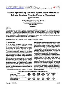
Fig. 1: Flow sheet of the modular continuous polymerization plant. (u1 , u2 , u3 and u4 ): side injections of monomer. The temperature of the reactor is controlled via the cooling/heating jacket (T). (T1 , T2 , T3 and T4 ): temperature measurements, Mw : molecular weight measurement (derived from a viscosity measurement). and assuming perfect mixing in the radial direction and negligible axial dispersion, a rigorous model of the reactor was set up. The free radical polymerization of acrylic acid is modeled by the terminal model approach. The resulting non-linear partial differential equations (pde) are shown in equations 1 to 8 (Hashemi et al. 2013). The temperature dependent rate coefficients kd (T ), kp (T ) and ktc (T ) are modeled by an Arrhenius approach and the method of moments is applied to model the polymer chain length distribution (Crowley et al. 1997).   ∂cI ∂t ∂cM ∂t ∂λ0 ∂t ∂λ1 ∂t ∂λ2 ∂t ∂µ1 ∂t ∂µ2 ∂t ∂T ∂t

∂cI ∂cI ∂ Dax − kd c I = −u + ∂z ∂z  ∂z  ∂cM ∂cM ∂ Dax − kp λ 0 c M = −u + ∂z ∂z ∂z   ∂λ0 ∂λ0 ∂ Dax + 2f kd cI − 2ktc λ0 2 = −u + ∂z ∂z ∂z ∂λ1 = −u + 2f kd cI + kp λ0 cM − ktc λ0 λ1 ∂z ∂λ2 = −u + 2f kd cI + kp cM (λ0 + 2λ1 ) − ktc λ0 λ2 ∂z ∂µ1 = −u + ktc λ0 λ1 ∂z ∂µ2 = −u + ktc λ0 λ2 + ktc λ1 2 ∂z   ∂T 2k ∂T ∂ λ = −u + (Tjac − T ) λ0 cM (−∆hp ) ∂z ∂z ∂z R

6

5

x 10

4 5000 points (simulation time: 204.84 [s]) 2000 points (simulation time: 48.43 [s]) 800 points (simulation time: 17.05 [s]) 400 points (simulation time: 10.08 [s]) 200 points (simulation time: 4.48 [s])

3 2 1 0 0 6 x 10 5

1000

2000

3000

4000

5000

6000

1000

2000

3000 Time [s]

4000

5000

6000

4

(1)

2

Module8

2

Product

µ [mol/m3]

QI Mw

µ2 + λ2 . (9) µ1 + λ1 Numerical methods have to be used to solve the pde model of the reactor system. Several methods have been introduced for this purpose in the literature. We employ the method of lines here. The main idea of this method is to replace all derivatives in the pde system by algebraic approximations except of one. Usually all spatial derivatives (dimensions) are approximated and do not appear explicitly in the model any more. Thus the pdes are converted to a system of odes. This method assigns an ode to every pde at each discretization point. Well-established methods for solving odes can then be applied to find the approximate solution of the original system of pdes. The standard choice to approximate the spatial derivatives is to use finite differences. Two major numerical issues result when implementing this method for processes with steep fronts, as the one considered here: A first order approximation of the spatial derivatives with finite differences results in numerical diffusion, i.e. smoothing of the fronts. This problem can be reduced by employing a fine discretization grid or by using higher order finite differences. Higher order approximations, however, result in numerical oscillations and the use of more discretization points does not reduce the numerical oscillations (Schiesser et al. 2009). Therefor, a first order approximation with a large number of discretization points must be used when finite differences are employed, leading to large computation times. Figure 2 illustrates these numerical problems. An alternative method is to use non-linear approximations of the spatial derivatives. The class of such non-linear approximation methods is called high resolution methods and includes flux limiters and weighted essentially nonoscillatory (WENO) methods (Bouaswaig et al. 2009). The latter one has been applied in this work and it was observed that both numerical problems can be avoided without the need for a fine discretization grid. WENO Mw =

µ [mol/m3]

jacket is used to control the reactor temperature and its temperature is set uniformly via a thermostat. Figure 1 shows the P&ID diagram of this reactor. The reactor is divided into four segments, each consisting of two modules, and a temperature sensor at the middle of each segment is installed. The internal volume of the first two segments is 45ml where segments three and four are larger and each has a volume of 130ml. A measurement of the viscosity measurement, is available at the outlet of the reactor which can be used to compute the average molecular weight Mw . Based on the energy and component balances

3 2 1

(2) (3) (4) (5) (6) (7) (8)

The weight average molecular weight of the produced polymer (Mw ) results from the moments as:

0 0

Fig. 2: Second moment of inactive polymers (µ2 ) at the reactor outlet. (a) First order finite differences are used to approximate the spatial domain in different discretization girds. This method results in numerical diffusion which can be avoided partly by fine discretization grids 1 . (b) High order finite differences are used to approximate the spatial domain. This method results in numerical oscillations which can not be cured by a finer discretization grid. schemes implement a dynamic set of stencils and compute a low order approximating polynomial in each of them to 1

4874

Intel(R) Core(TM) i7-2600 CPU @ 3.40GHz, 24GB RAM

19th IFAC World Congress Cape Town, South Africa. August 24-29, 2014

compute the numerical flux. Each polynomial receives a weight which is determined based on a local smoothness indicator. The polynomials corresponding to the stencils which have a large gradient receive a zero weight giving a non-oscillatory solution at the sharp fronts. The obtained polynomials are combined in a non-linear convex fashion, resulting in higher order polynomials at the smooth parts of the solution and in an upwind spatial discretization at the sharp fronts which avoids interpolation and provides the necessary dissipation for shock capturing (Borges et al. 2008). The spatial derivatives then are approximated by a first order finite difference of the computed numerical flux. Different variants of WENO schemes devise different smoothness indicators and determine the weights of polynomials in different ways. In this work, we have implemented the WENO-Z scheme proposed by (Borges et al. 2008). The details about the determination of the smoothness indicators and weights can be found in their work. The second derivatives of the spatial domain that appear in the process model can be rewritten by means of two first order derivatives using auxiliary variables. Then the current WENO scheme can be used to compute the second derivatives. (Liu et al. 2011) have proposed a new WENO scheme to compute the second derivatives directly. Their scheme has a higher resolution and we have implemented their method in our model. The advantage of using the WENO scheme can be seen in figure 3. A Matlab implementation of the model with the WENO scheme with 200 discretization points needs only 66.71 seconds and can reach a similar accuracy as the finite differences with 5000 discretization points which takes 204.84 seconds 2 . For the rest of this paper, we will use the WENO scheme with a uniform discretization grid of 200 points. The obtained ode model, which includes 1600 states, is solved using the CVode from the Matlab interface of SUNDIALS (sundialsTB).

Also in case of the availability of the suitable sensors, the measurements are always noisy. The extended Kalman filter (EKF) is the most widely used state estimation technique for non-linear systems in the process industries. It employs a prediction step using the non-linear model and a correction step using the available measurements. The Kalman gain matrix is computed based on a linearization of the system around the previous estimate (Simon 2006). The extended Kalman filter usually provides a satisfactory performance if the non-linearities of the system are not too severe otherwise it can show poor performance or become unstable. The performance of EKF is strongly dependent on its tuning, a task which can be quite difficult for large systems. We have implemented the extended Kalman filter for this reactor and observed that it indeed became unstable for quite reasonable tuning parameters (results are not shown here). In this work, we apply the particle filtering (PF). Particle filters are recursive sample based state estimation algorithms which employ the full model of the system. They start with a given number of initial guesses of the a priori states (particles). Based on the probability of the current measurements resulting from these particles as a posteriori states, the algorithm assigns a weight to each of them. Finally an a posteriori set of particles is chosen and the mean value of this set is considered as the final estimation of the current state. Particle filters do not need assumptions about the type of model of the system (linear or nonlinear) nor about the distribution of the assumed measurement and process noise. Any suitable system model or noise probability density function can be used. A generic particle filtering algorithm can be described in the following steps (Arulampalam et al. 2002):

6

4.5

x 10

4 Finite Difference with 5000 discretization points WENO with 200 discretization points 3.5

3

µ [mol/m ]

3

2

2.5 2 1.5 1 0.5 0

1000

2000

3000 Time [s]

4000

5000

6000

Fig. 3: Second moment of inactive polymers (µ2 ) at the outlet of the reactor. 3. PARTICLE FILTERS State estimation is an important part of every control scheme. While the prediction of the behavior of a given system requires the knowledge of the initial states, usually not all states of the system can be measured or some quantities can not be measured at the requested frequency.

(0) The process and observation equations are given as follows:  xk = fk (xk−1 , uk−1 ) + ωk−1 , yk = hk (xk ) + υk , (10)  x(0) = x0 + ω0 .

where ω and υ are the process and measurement noise and are white noise signals with known probability density functions (pdf) and mutually independent. We assumed here that the measurements of the temperature and of the molecular weight contain Gaussian noise with standard deviations of 0.2 [K] and 1 [kg/mol]. The process noise also obeys a Gaussian distribution and is assumed to have a standard deviation of about 0.1% of the range of the states. (i) From the pdf of the initial states N random particles are generated. In our case N = 1000. Each particle receives an importance weight equal to N1 . The distribution of the monomer concentrations along the reactor for the initial particles (estimates) and for one simulation run is shown in figure 4. (ii) The particles that were generated in the previous step are propagated via the system model (eq.10). (iii) The algorithm updates the weights of the particles (for a scalar measurement for simplicity) as follows:

2

The stated simulation times are measured when the Matlab integrator ode15s has been used. The designed NMPC, uses a mex implementation of the model and employs CVode from sundialsTB which increases the simulation speed with a factor of 100.

4875

i∗ wki = wk−1 ·

p(yk |xik ) · p(xik |xik−1 ) q(xik |xik−1 , yk )

(11)

where q(.) is the importance density function. “k” refers to the time instants and “i” is the counter of

19th IFAC World Congress Cape Town, South Africa. August 24-29, 2014

the particles. The superscript “*” denotes the scaled weights. If more than one state is measured, the joint likelihoods have to be computed. The weights are scaled so that the sum of all weights equals one. ωi ωki∗ = PN k j (12) j=1 ωk Particle filters can suffer from the degeneracy problem which means that after a few iterations, it is possible that all particles except a few have a very small weight. In such a situation, the set of particles will lose its diversity and it can not represent the likelihood density function of the states anymore. A suitable measure of the degeneracy of the set of particles is the effective sample size (Nef f ). An estimation of the effective sample size is: ˆef f = P 1 (13) N N i∗ 2 j=1 (ωk ) ˆef f is less than a given value, resampling is If N performed. A small effective sample size indicates severe degeneracy. A set of a posteriori particles is chosen. This process is called resampling and there are various methods for it. The four most often applied methods are multinomial, residual, stratified and systematic resampling. In this work, we have tested the multinomial and systematic methods and observed better results from the systematic approach. (Arulampalam et al. 2002) and (Doucet et al. 2008) have also reported a better performance of the systematic method over the other methods. The systematic resampling method can be summarized in the following way: Sample Ui = U1 + i−1 N, U1 ∼ U [0, N1 ] and N for i = 2, ..., o n define Pi P j−1 i k k then set Nn = Uj : k=1 Wn ≤ Uj ≤ k=1 Wn . The n selected set of the aoposteriori particles is: PN Nni π ¯= i=1 N δ(x − xi ) (Doucet et al. 2008). Resampling can drop some of the particle and select some of them twice or more. Any statistical measure of the a posteriori set can be computed. Usually the mean value is of interest.

shown in figure 6. For this simulation all five available measurements have been used. The RMS of the estimation error of the molecular weight at the outlet (Mw ) and monomer concentration (CM ) are 0.0601 and 1.5976. The choice of the initial particles has to be in accordance with the measurement error. Small measurement noise requires precise initial particles. The reason for this can be explained as follows: The algorithm propagates the particles and computes the predictions of the variables which are measured. Then the importance weights are assigned based on the proximity of these values to the measured ones. If the initial particles are chosen too far away from the true states, they produce values which are far from the measured ones and the algorithm will disqualify all of them.

Several variants of particle filters exist which vary in the choice of the importance sampling density function or in the resampling step. In this work we have implemented the Sequential Importance Resampling (SIR) filter which does the resampling at every step and defines the importance sampling density function as follows: q(xik |xik−1 , yk ) = p(xk |xik−1 ) (14) Since the resampling is performed at every time instant, the weights of the particles are (Arulampalam et al. 2002): ωki = p(yk |xik ) (15) The SIR algorithm is the most widely used version of particle filtering since the importance weights can be easily evaluated. However it is sensitive to outliers. A simulation result obtained with this method is presented in figure 5. No model-plant mismatch is considered in this simulation. The distribution of the true initial monomer concentration along the reactor and the distribution of the monomer concentration of all 1000 initial particles are shown in figure 4. The manipulated variables for this simulation are

Fig. 5: (a) True, measured and estimated molecular weight at the outlet of the reactor, (b) true and estimated monomer concentration at the outlet of the reactor.

3

CM [mol/m ]

1000

800

600

400

200

0 0

0.5

1

1.5

2 length of reactor [m]

2.5

3

3.5

4

Fig. 4: Distribution of the monomer concentrations of the initial particles and of the true concentration along the reactor.

M [kg/mol]

80 true measured estimated

w

75

70

true estimated

3

C [mol/m ]

250

M

200

150

100 0

0.5

1

1.5

2 Time [s]

2.5

3

3.5

4 4

x 10

100

400

u

u

2

u

3

u

4

T

4

1

3

50

0 0

380

0.5

1

1.5

2 Time [s]

2.5

3

T [K]

(vii)

paricles true 1200

2

(vi)

1400

1

(v)

Side injections of monomer (u , u , u , u ) [%]

(iv)

360 4

3.5

4

x 10

Fig. 6: Manipulated variables for the simulation of the state estimation shown in figure 5.

4876

19th IFAC World Congress Cape Town, South Africa. August 24-29, 2014

4. OPTIMIZING CONTROL 4.1 Non-linear Model Predictive Control The reactor in this work is controlled by a model-based optimizing controller i.e. the control moves are optimized over a finite horizon considering the predicted response of the plant and the constraints on the product properties. Standard implementations of NMPC employ tracking cost functions and penalize the violations of the outputs or states from a given set point (Findeisen et al. 2004). In this work we follow the idea of online optimizing control and aim at maximizing the product throughput under the quality constraints (Engell 2007). For the reactor shown in figure 1, the product throughput is maximized when the sum of all flow rates of the monomer side injections are maximized, but the quality constraints have to be fulfilled. The residual monomer (CM ) is an important product quality indicator and is estimated at the outlet of the reactor. The second product quality constraint is imposed on the molecular weight that is measured indirectly at the outlet of the reactor (Mw ). These constraints can be formulated as hard constraints which is computationally more demanding but then the quality constraints are strictly met. In this work we deal with these constraints as soft constraints and penalize their violations from the considered bounds in the cost function. This is based on the assumption that the produced polymer will be sold in larger quantities hence a considerable degree of mixing occurs after the production and smoothens short-term constraint violations. Following this idea, the cost function is formulated as follows: min Φ(x(tk ), u(tk ), Nc , Np ) (16a) u1k ,u2k ,u3k ,u4k ,Tk

Φ = −Φ1 + γΦ2 = −Φ1 + γ (Φ21 + Φ22 + Φ23 ) (16b) j=k+Np

Φ1 =

X

(u1 + u2 + u3 + u4 )

(16c)

(max(CM j − CM u , 0))2

(16d)

(max(Mwj − Mwu , 0))2

(16e)

(min(Mwj − Mwl , 0))2

(16f)

j=k

j=k+Np

Φ21 =

X j=k

j=k+Np

Φ22 =

X j=k

j=k+Np

Φ23 =

X j=k

where the subscripts l and u denote the lower and upper bounds of the corresponding variables. Np and Nc are the length of prediction and control horizons. The residence time of the reactor for the nominal flow rate is about 2600 seconds which implies that the prediction horizon must be at least of a similar length. However, the controller manipulates the total flow rates inside the reactor, causing a shift in the states which postpones or expedites the effect of a specific control move depending on the previous control move. In order to take this behavior into account and to ensure a stable behavior, we use a prediction horizon of 6000 seconds which in this case is a quasi-infinite horizon. The control horizon is set to one to reduce the number of the decision variables. The sampling time is 100 seconds. The first part of the cost (Φ1 ) maximizes the

product throughput while the second part (Φ2 ) minimizes the violations of the controlled variables from the given bounds. γ is a tuning parameter and determines the relative importance of Φ1 and Φ2 in the computed cost. From a numerical point of view, this formulation of the cost function is easier to solve because it does not include explicit constraints. The reactor temperature (T) does not enter into the optimization problem directly but it is manipulated to fulfill the constraints and to enable an increase of the throughput. The optimization problem is solved in a sequential approach using the SNOPT solver from the TOMLAB package. In each sampling instant, the initial condition of the model is estimated employing the particle filter that was introduced in the previous section. 4.2 Simulation Results In this section we show the application of the optimizing controller to the tubular polymerization reactor while a particle filter is used to estimate the initial states of the prediction model. For the base design case (no regulation), the produced polymer has a molecular weight of 77.5 [kg/mol] and a monomer content of about 131 [mol/m3 ] at the reactor outlet. The following choices of the bounds in (16d − 16f ) were made: CM u = 135, Mwl = 75, Mwu = 80 We assume that the reactor initially is in steady state and produces the requested polymer with the base-design inputs. At t = 0, the controller is switched on. Considering the normalization of the constructing elements of the cost function (Φ1 and Φ2 ), we have set the tuning parameter γ to 0.02. The computed manipulated variables by the optimizing controller are shown in figure 7. Compared to the base design case, the controller increases the throughput by 49.0%. As shown in figure 8, the estimated variables converge to the true values and the controlled variables are kept within the specified bounds. The small violations from the bounds in the transition phase result from the application of soft constraints. The controller drives the reactor to an operation at a higher temperature as expected and increases the side injections of monomer considerably. This system has a very complex behavior and does not exhibit a monotonically increasing or decreasing step response. This is the main reason for the fluctuation of the controlled variables before reaching a steady state. The implemented code of the controller has been partially parallelized to apply parallel computation. For the process and measurement noise, the same assumptions as for the simulation in section 3 were made here. The computation times of the optimizing controller and of the particle filter for this simulation are shown in figure 9. 5. CONCLUSION We demonstrated the application of model-based optimizing control to a challenging reactor control example. The investigated process is the continuous polymerization of acrylic acid in a tubular reactor with multiple side injections of monomer. The spatial domain of the pde model was discretized and the spatial derivatives were computed using the WENO scheme. We implemented an economical cost function which aims directly at maximizing the product throughput. The product and quality constraints

4877

ever, as the propagation of each particle is independent from the other particles, parallel computation can be applied. With the particle filter estimator, the controller can meet the specifications of the controlled variables and increases the product throughput considerably. A drawback of the optimizing controller is its long computation times. Reduced or simplified models could be used to reduce the simulation time of the model. Consideration of parametric inaccuracies besides the measurement and process noises will be a further extension of this work.

150 u

u

1

2

u

3

u

4

Total Flow

100

2

3

4

Side injections of monomer (u , u , u , u ) [%]

19th IFAC World Congress Cape Town, South Africa. August 24-29, 2014

1

50

0 395

T [K]

390

385

ACKNOWLEDGEMENTS

380 0

0.2

0.4

0.6

0.8

1 Time [s]

1.2

1.4

1.6

1.8

2 4

x 10

Fig. 7: Manipulated variables computed by the optimizing controller. 3

C (@ outlet) [mol/m ]

140 true estimated

120

M

100 80

We would like to gratefully acknowledge the contribution of Daniel Kohlmann from the Process Dynamics and Operations Group at TU Dortmund to the modeling of the process investigated in this work. This work was supported by the European Union within the project F3 Fast Flexible Future Factory and by the ERC Advanced Investigator Grant MOBOCON awarded to the second author.

w

M (@ outlet) [kg/mol]

60 84

REFERENCES

82 80 true measured estimated

78 76 74 72 0

0.2

0.4

0.6

0.8

1 Time [s]

1.2

1.4

1.6

1.8

2 4

x 10

Fig. 8: Controlled variables of the system under optimizing controller. A particle filter is employed to provide the initial conditions of the prediction model. Computation time of optimizing control [s]

800 600 400 200

Computation time of particle filter [s]

0 30 25 20 15 10 5 0 0

20

40

60

80

100 120 Iteration number

140

160

180

200

Fig. 9: (a) Computation times of the optimizing controller. (b) Computation times of the implemented particle filter with 1000 particles. In this simulation the parallel computation facility of Matlab with 12 workers has been used. are considered as soft constraints and enter into the cost function. In order to provide the initial conditions of the prediction model a state estimator must be implemented. State estimation in tubular reactors is a difficult task because compared to the number of the states, the available measurements are scarce. In this work we assumed four temperature measurements along the reactor and one molecular weight measurement at the reactor outlet. The state estimation was performed using a particle filtering algorithm. The advantage of particle filtering over the extended Kalman filter is that it utilizes the full non-linear model of the process and does not encounter the problems resulting from linearization. Usually the computation time of the particle filters is considered as their drawback. How-

W.E. Schiesser, G.W. Griffiths. (2009) A Compendium of Partial Differential Equation Models: Method of Lines Analysis with Matlab Cambridge University Press. ISBN 9780521519861. R. Borges, M. Carmona, B. Costa, W.S. Don, (2008). An improved weighted essentially non-oscillatory scheme for hyperbolic conservation laws Journal of Computational Physics 227, 3191–3211. Y. Liu, C.-W. Shu, M. Zhang. High order finite difference WENO schemes for non-linear degenerate parabolic equations SIAM J. Sci. Computer. 33 (2011) 939-.965. R. Hashemi, D. Kohlmann, S. Engell (2013). Optimizing Control of a Continuous Polymerization Reactor. 10th international symposium on dynamics and control of process systems (DYCOPS) , 2013. S. Engell (2007). Feedback Control for Optimal Process Operation Journal of Process Control 17(3), 203–219, 2007. R. Findeisen, F. Allg¨ower, M.C. Nagy (2004). Nonlinear Model Predictive Control: From Theory to Application J. Chin. Inst. Chem. Engrs., 35, 3, 299–315, 939–965. D. Simon. (2006) Optimal State Estimation, Kalman, H∞ and nonlinear approaches John Willy & Sons, Inc., Hoboken, New Jersey. M.S. Arulampalam, S. Maskell, N. Gordon, T. Clapp (2002). A Tutorial on Particle Filters for Online Nonlinear/Non-Gaussian Bayesian Tracking. IEEE Transactions on signal processing , 50, NO.2, 174–188. S. Russell, P. Norvig (2003) Artificial Intelligence: A Modern Approach Upper Saddle River, New Jersey: Prentice Hall A. Doucet, A.M. Johansen (2008) A Tutorial on Particle Filtering and Smoothing: Fifteen years later version 1.1 A.E. Bouaswig, S. Engell (2009) WENO scheme with static grid adaptation for tracking steep moving fronts Journal of Chemical Engineering Science, 64 (2009) 3214–3226 T.J. Crowley, K.Y. Choi (1997) Calculation of Molecular Weight Distribution from Molecular Weight Moments in Free Radical Polymerization Ind. Eng. Chem. Res. , 1997, 36, 1419–1423

4878