Overview of PCA-Based Statistical Process-Monitoring Methods ... - ASQ

Overview of PCA-Based Statistical Process-Monitoring Methods for Time-Dependent, High-Dimensional Data BART DE KETELAERE*, MIA HUBERT**, and ERIC SCHMITT** Leuven Statistics Research Centre, KU Leuven, Celestijnenlaan 200B, B-3001 Heverlee, Belgium

*Department of Biosystems, Division MeBioS, KU Leuven, Kasteelpark Arenberg 30, B-3001 Heverlee, Belgium **Department of Mathematics, KU Leuven, Celestijnenlaan 200B, B-3001 Heverlee, Belgium High-dimensional and time-dependent data pose significant challenges to statistical process monitoring. Dynamic principal-component analysis, recursive principal-component analysis, and moving-window principal-component analysis have been proposed to cope with high-dimensional and time-dependent features. We present a comprehensive review of this literature for the practitioner encountering this topic for the first time. We detail the implementation of the aforementioned methods and direct the reader toward extensions that may be useful to their specific problem. A real-data example is presented to help the reader draw connections between the methods and the behavior they display. Furthermore, we highlight several challenges that remain for research in this area. Key Words: Autocorrelation; Nonstationarity; Principal-Component Analysis.

able to cope with these process types and indicate some advantages and disadvantages. A wide range of scenarios encountered in SPM have motivated the development of many control-chart techniques, which have been improved and reviewed over the course of the last 40 years. Bersimis et al. (2006) give an overview of many multivariate process-monitoring techniques, such as the multivariate EWMA and multivariate CUSUM, but provide minimal coverage of techniques for high-dimensional processes. Barcel´ o et al. (2010) compare the classical multivariate timeseries Box–Jenkins methodology with a partial least squares (PLS) method. The latter is capable of monitoring high-dimensional processes, but more methods for a broader range of time-dependent process scenarios are not covered. In discussing the monitoring of multivariate processes, Bisgaard (2012) highlights principal-components analysis (PCA), partial least squares, factor analysis, and canonical correlation analysis as applicable monitoring methods. These methods and their extensions have the property that they are capable of handling high-dimensional process data and time-dependence. All of them project the high-dimensional process onto a lower dimen-

1. Introduction are a widely used tool, Q developed in the field of statistical process monitoring (SPM) to identify when a system is deviUALITY CONTROL CHARTS

ating from typical behavior. High-dimensional, timedependent data frequently arise in applications ranging from health care, industry, and IT to the economy. These data features challenge many canonical SPM methods, which lose precision as the dimensionality of the process grows, or are not wellsuited for monitoring processes with a high degree of correlation between variables. In this paper, we present an overview of foundational principalcomponent analysis-based techniques currently availDr. De Ketelaere is Research Manager in the Division of Mechatronics, Biostatistics and Sensors (MeBioS). His email is [email protected]. Dr. Hubert is Professor in the Department of Mathematics. Her email is [email protected]. Mr. Schmitt is Doctoral Student in the Department of Mathematics. His email is [email protected]. He is the corresponding author.

Journal of Quality Technology

318

Vol. 47, No. 4, October 2015

OVERVIEW OF PCA-BASED PROCESS MONITORING OF TIME-DEPENDENT HIGH-DIMENSIONAL DATA

sional subspace and monitor the process behavior with respect to it. Woodall and Montgomery (2014) provide a survey of multivariate process-monitoring techniques as well as motivations for their use. The authors also provide clear insights into possible process types and which monitoring methods might be suitable and o↵er commentary on popular performance measures, such as the average run length and false discovery rate. Other books and papers devote more attention to PCA process monitoring. Kourti (2005) describes fundamental control charting procedures for latent variables, including PCA and PLS, but does not discuss many of the main methods for time-dependent data nor their extensions. Kruger and Xie (2012) include a chapter covering the monitoring of high-dimensional, time-dependent processes but focus on one method only. Qin (2003) provides a review of fault detection, identification and reconstruction methods for PCA process monitoring. He mentions the challenges of monitoring time-dependent processes, but restricts his primary results to cases where the data is not time dependent. However, to the best of our knowledge, an overview directly focusing on the range of available control chart techniques concerned with high-dimensional, time-dependent data has not yet been written with directions for practical use. We assume that we have observed a large number, p, of time series xj (ti ), (1  j  p) during a calibration period t1 , t2 , . . . , tT . As time continues, more measurements become available. SPM aims to detect deviations from typical process behavior during two distinct phases of process measurement, called phase I and phase II. Phase I is the practice of retrospectively evaluating whether a previously completed process was statistically in control. Phase II is the practice of determining whether new observations from the process are in control as they are measured. Two types of time dependence are autocorrelation and nonstationarity. Autocorrelation arises when the measurements within one time series are not independent. Nonstationarity arises when the parameters governing a process, such as the mean or covariance, change over time. While it can be advantageous to include process knowledge, such as information about normal state changes, for the sake of focus, we will assume no such prior knowledge. When no autocorrelation is present in the data and the process is stationary, control charts based on PCA have been successfully applied in processmonitoring settings with high dimensionality. These


319

methods operate by fitting a model on a T ⇥ p calibration data matrix XT,p , where the ith row in the jth column contains the ith measurement of the jth time series xj (ti ) for 1  i  T . The number of rows of XT,p thus refers to the number of observed time points and the number of columns to the number of time series measured in the system. The calibration data are chosen to be representative of typical behavior of the system. A new observation at time t, x(t) = (x1 (t), x2 (t), . . . , xp (t))0 , is compared with the data in XT,p , and evaluated by the control chart to determine whether it is typical. This is called static PCA because the fitted model remains static as new observations are obtained. Therefore, it will not adjust as underlying parameter values change (nonstationarity) and no attempt is made to model relationships between observations at di↵erent time points (autocorrelation). One can identify autocorrelation in a process by examining autocorrelation and cross-correlation functions of the data, as we shall do below. Nonstationarity can be assessed on univariate data using the augmented Dickey–Fuller test for a unit root. In high-dimensional data, a compromise is to perform this test on each of the scores of a static PCA model. Three classes of approaches have been proposed to extend PCA methods to cope with time-dependant data. These are dynamic PCA (DPCA), recursive PCA (RPCA), and moving-window PCA (MWPCA). DPCA was developed to handle autocorrelation, whereas RPCA and MWPCA are able to cope with nonstationary data. No method is currently proposed for settings when both autocorrelation and nonstationarity are present. Although existing methods may provide acceptable monitoring in some contexts, this is nonetheless an area for further research.

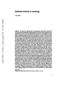
2. Introducing the NASA Bearings Data Set Throughout this paper, the NASA Prognostics Center of Excellence bearing data set (Lee et al. (2007)) will be used to illustrate the behavior of the methods on data with autocorrelation and nonstationarity. As shown in Figure 1, the data consist of measurements of eight sensors (p = 8), with each sensor representing either the x or y-axis vibration intensities of a bearing. Four bearings are monitored at intervals of approximately 15 minutes, and a vibration signal of about a second is recorded to describe the “stability”. These raw data are then compressed into a single feature for each sensor. The resulting

www.asq.org

320

BART DE KETELAERE, MIA HUBERT, AND ERIC SCHMITT

FIGURE 1. Data Series Depicting the Autocorrelated, Nonstationary NASA Ball-Bearing Data Set. Sensors 7 and 8 are plotted in light gray. Other sensors are plotted in dark gray.

observations are eight-dimensional vectors of bearing vibration intensities spaced at approximately 15minute intervals. These are paired such that the first two sensors correspond to the first bearing and so on. Figure 1 shows that there are two variables, belonging to the seventh and eighth sensors corresponding to the fourth bearing (plotted in light gray), which begin to deviate from typical behavior shortly after the 600th observation. Later in the experiment, a catastrophic failure for all of the bearings is observed. The NASA process shares many similarities with a multistream process (MSP). An MSP results in multiple streams of output for which, from the perspective of SPM, the quality variable and its specifications are identical across all streams. An MSP may also be defined as a continuous process where multiple measurements are made on a cross section of the product (Epprecht et al. (2011)). The NASA process has features of both of these definitions. It resembles the first in the sense that each of the bearings may be seen as having similar specifications to one another, with the average vibrations tending to be slightly different (but this can be adjusted so that they have the same mean), and the displayed variance being similar. The NASA process resembles the second definition in the sense that multiple measurements are made on a cross section of the process; namely, all of the bearings are measured by two sensors. We detect some correlation between the streams, but as Epprecht and Sim˜ oes (2013) note, this violates the assumption, made by most MSP methods, that none is present. Given these process features, PCA and its


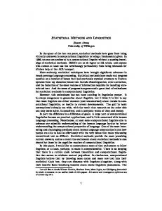
FIGURE 2. Histograms, Scatterplots, and Correlations of Sensors 1, 2, 7, and 8 During the First 120 Measurements.

extensions are a possible monitoring solution. Runger et al. (1996) applied PCA to MSPs and note that this approach models the correlation structure between process variables. PCA is also capable of monitoring more general multivariate processes consisting of outputs that do not have identical properties, which may be the case when the second MSP definition is more appropriate and multiple measurements are made on a cross section. An additional advantage of PCA is that it is capable of modeling high-dimensional processes, which can pose problems for many MSP methods requiring an invertible covariance matrix. Histograms, correlations, and pairwise scatterplots of vibration intensity measurements from sensors (1 and 2) placed on a typical bearing and sensors (7 and 8) on a deviating bearing are presented in Figure 2 for the first 120 observations, as these exhibit behavior characteristic of the in-control process. The corresponding autocorrelation functions (ACFs) up to 50 lags are depicted in Figure 3. The autocorrelation is presented as light-gray bars, while a limit to identify lags with high autocorrelation is expressed as a dark-gray line. During this early period, the pairs of sensors are only mildly correlated, with autocorrelation only exceeding the dark-gray line indicating the 97.5 percentile limits for a few lags. For comparative purposes, the descriptive plots and autocorrelation functions are also shown for observations between



321

FIGURE 3. ACFs of Sensors 1, 2, 7, and 8 During the First 120 Measurements.

FIGURE 5. ACFs of Sensors 1, 2, 7, and 8 During the Time Period Between t = 600 and t = 1,000.

t = 600 and t = 1000 in Figures 4 and 5. In the plots for the later time period, we see that sensors 7 and 8 become highly correlated as failure occurs. An advantage of multivariate control charts is that they take the change in the correlation between variables into account when determining if a system is going out of control. Furthermore, because nonstationarity has begun to develop, the ACFs now report very high-order autocorrelation. Earlier observations will be used to fit models, but control charts will also be used to assess these observations. In our context,

we will consider this monitoring phase I because it could be used by the practitioner to gain a better understanding of the behavior of this process from historical data. For the purposes of this paper, we will consider the later observations to be absent from the historical observations the practitioner could access for phase I monitoring and thus monitoring these later observations will constitute phase II.

3. Static PCA 3.1. Method Principal-components analysis defines a linear relationship between the original variables of a data set, mapping them to a set of uncorrelated variables. In general, static PCA assumes an (n ⇥ p) data matrix Xn,p = (x1 , . . . , xn )0 . Let 1n = (1, 1, . . . , 1)0 be of length n. Then the mean can be calculated 0 ¯ = (1/n)Xn,p as x 1n and the covariance matrix as ¯ 0 )0 (Xn,p 1n x ¯ 0 ). Each pS = [1/(n 1)](Xn,p 1n x dimensional vector x is transformed into a score vec¯ where P is the p ⇥ p loading mator y = P 0 (x x), trix, containing column-wise the eigenvectors of S. More precisely, S can be decomposed as S = P ⇤P 0 . Here, ⇤ = diag( 1 , 2 , . . . , p ) contains the eigenvalues of S in descending order. Throughout this paper, PCA calculations will be performed using the covariance matrix. However, it is generally the case that the methods discussed can also be performed using the correlation matrix R by employing di↵erent formulas.

FIGURE 4. 4.Histograms, Scatterplots, and Correlations of Sensors 1, 2, 7, and 8 During the Time Period Between t = 600 and t = 1,000.


It is common terminology to call y the scores and the eigenvectors, P , the loading vectors. In many cases, due to redundancy between the vari-

www.asq.org

322


ables, fewer components are sufficient to represent the data. Thus, using k < p of the components, one can obtain k-dimensional scores by the following: y = Pk0 (x

¯ x),

(1)

where Pk contains only the first k columns of P . To select the number of components to retain in the PCA model, one can resort to several methods, such as the scree plot or cross validation. For a review of these and other methods, see, e.g., Valle et al. (1999) and Jolli↵e (2002). In this paper, the number of components will be selected based on the cumulative percentage of variance (CPV), which is a measure of how much variation is captured by the first k PCs and is Pk j=1 CPV(k) = Pp j=1

j

100%.

j

The number of PCs is selected such that the CPV is greater than the minimum amount of variation the model should explain. Control charts can be generated from PCA models by using the Hotelling’s T 2 statistic and the Q-statistic, which is also sometimes referred to as the squared prediction error (SPE). For any pdimensional vector x, Hotelling’s T 2 is defined as T 2 = (x

¯ 0 Pk ⇤k 1 Pk0 (x x)

¯ = y 0 ⇤k 1 y, x)

where ⇤k = diag( 1 , 2 , . . . , k ) is the diagonal matrix consisting of the k largest eigenvalues of S. The Q-statistic is defined as Q = (x

¯ 0 (I x)

Pk Pk0 )(x

¯ = kx x)

ˆ 2, xk

ˆ = Pk Pk0 (x x). ¯ The Hotelling’s T 2 is the with x Mahalanobis distance of x in the PCA model space and the Q-statistic is the quadratic orthogonal distance to the PCA space. Assuming temporal independence and multivariate normality of the scores, the 100(1 ↵)% control limit for Hotelling’s T 2 is T↵2 =

k(n2 n(n

1) Fk,n k)

k (↵).

where ✓i =

p X

j=k+1

i j

for i = 1, 2, 3 and h0 = 1

2✓1 ✓3 3✓22

and z↵ is the (1 ↵) percentile of the standard normal distribution. Another way of obtaining cut-o↵s for the Q-statistic based on a weighted 2 distribution is detailed in Nomikos and MacGregor (1995). An advantage of this approach is that it is relatively fast to compute. During phase I, the T 2 - and Qstatistic are monitored for all observations x(ti ) = (x1 (ti ), . . . , xp (ti ))0 with 1  i  T . It is important to note that fitting the PCA model to these data will result in a biased model with possible inaccurate fault detection if faults are present because they can bias the fit. If faults are present, it is advised to fit a robust PCA model and refer to the monitoring statistics it produces. Phase II consists of evaluating contemporary observations xt = x(t) using the T 2 and Q-statistic based on the outlier-free calibration set. An intuitive depiction of static PCA is given in Figure 6. This figure will serve as a basis of comparison between the DPCA, RPCA, and MWPCA techniques that are discussed in the following sections. Variables are represented as vertical lines of dots measured over time. The light-gray rectangle contains the observed data during the calibration period that is used to estimate the model that will be used for subsequent monitoring. The dark-gray rectangle is the new observation to be evaluated. The two plots

(2)

Here, Fk,n k (↵) is the (1 ↵) percentile of the F distribution with k and n k degrees of freedom. If the number of observations is large, the control limits can be approximated using the (1 ↵) percentile of the 2 distribution with k degrees of freedom, thus T↵2 ⇡ 2k (↵). The simplicity of calculating this limit is advantageous. The control limit corresponding to the (1 ↵) percentile of the Q-statistic can be calculated, provided that all the eigenvalues of the matrix S can


be obtained (Jackson and Mudholkar, 1979), as !2 p z↵ 2✓2 h20 ✓2 h0 (1 h0 ) +1+ , Q↵ = ✓1 ✓1 ✓12

FIGURE 6. A Schematic Representation of Static PCA at Times t (Left) and t + 1 (Right). The model is fitted on observations highlighted in light gray. The new observation, highlighted in dark gray, is evaluated.



show that, at time t + 1 (right), the same model is used to evaluate the new observation in dark gray as in the previous time period, t (left). PCA is well suited for monitoring processes where the total quality of the output is properly assessed by considering the correlation between all variables. However, if a response variable is also measured and the relationship of the process variables to it is of primary interest, the technique of partial least squares (PLS) is preferred to PCA. Like linear regression, it is used to model the linear relation between a set of regressors and a set of response variables; but like PCA, it projects the observed variables onto a new space, allowing it to cope with high-dimensional data. Control charts may be implemented for PLS in much the same way as they are for PCA. Kourti (2005) provides a comparison of PCA and PLS, as well as some references for PLS control chart literature. Static PCA requires a calibration period to fit a model. However, it is well known that PCA is highly susceptible to outliers. If outliers are included in the data used to fit a monitoring model, the detection accuracy can be severely impaired. Robust PCA methods, such as ROBPCA (Hubert et al. (2005)), have been designed to provide accurate PCA models even when outliers are present in the data. A robust PCA method can be used to identify outliers in the calibration data for removal or examination. Once these are removed, the resulting robust PCA model can be used as the basis for subsequent process monitoring. ROBPCA may be performed using the robpca function in the LIBRA toolbox (Verboven and Hubert (2005)) or the PcaHubert function in the R package rrcov (Todorov and Filzmoser (2009)). In addition to outliers, future observations with missing data and observations with missing data during the calibration phase present challenges for process monitoring. In the context of PCA control charts, a number of options for addressing these issues exist. The problem of future observations with missing data is typically addressed by using the process model and nonmissing elements of the new observation, xnew , to correct for the missingness of some of its elements. Examples of algorithms using this approach at various levels of complexity are discussed in Arteaga and Ferrer (2002). They conclude that a method referred to as trimmed score regression (TSR) has the most advantages, in terms of accuracy and computational feasibility, of the methods they considered. TSR uses information from the full


323

score matrix Y from the calibration data, the loadings in P corresponding to the nonmissing variables in xnew , and xnew itself to estimate the ynew . In the event that the calibration data have missing values, one does not have access to existing estimates of P and Y to use for missing-data corrections. Walczak and Massart (2001) propose a method for missingdata imputation based on the expectation maximization (EM) algorithm. Serneels and Verdonck (2008) make this method robust, allowing missing-data imputation to proceed even when the calibration data set is contaminated by outliers. An implementation is available in the rrcovNA package (Todorov (2013)) in R (R Core Team (2014)). 3.2. Static PCA Applied to the NASA Data In this subsection, we apply static PCA to the NASA data. Before constructing control charts, we performed ROBPCA on the first 120 observations that we use to fit the PCA model. No significant outliers were detected, so we fit a PCA model on that data without removing observations. No data were missing in this data set, so missing data methods were not employed. It is common in many fields to perform preprocessing. The type of preprocessing is typically determined by the type of process being monitored, with chemometrics, for instance, giving rise to many preprocessing approaches specific to that context. In the case of the NASA data, no special preprocessing is necessary. Since all of the sensors in the NASA data are measuring vibrations in the same units, standardizing the data is not strictly necessary.

FIGURE 7. Static PCA Control Charts for the Entire NASA Data Set. The first 120 observations are used to fit the underlying model.

www.asq.org

324

BART DE KETELAERE, MIA HUBERT, AND ERIC SCHMITT TABLE 1. Loadings of the Static PCA Model of the NASA Data

Component

FIGURE 8. ACFs of the First Two Scores of Static PCA Applied to the NASA Data Set for t  120.

Static PCA applied to the NASA bearing data set generates the control chart in Figure 7 and ACF plot in Figure 8. We plot the logarithm of the T 2 and Q-statistics in these and subsequent charts as solid light-gray lines and the control limit in solid, dark-gray lines. The first 120 observations are used to fit the underlying model, as we do not observe any large change in the vibration intensity of any of the sensors during this period, and this will also allow us to evaluate the estimated model against the well-behaved data observed before t = 120. Therefore, we di↵erentiate between phase I, which takes place when t  120, and phase II. A vertical line divides these two periods in Figure 7. Five components are retained in accordance with the CPV criterion. We see that failure of the system is detected before catastrophic failure occurs, at around t = 120 by the Q-statistic and at around t = 300 by the T 2 -statistic. Because we did not detect any major outliers using ROBPCA during phase I, it is not surprising that few observations exceed the cut-o↵s during this early period and that later, during phase II when the issue with the fourth bearing develops, we find a failure. Figure 8 shows there is room to reduce the variability of the statistics by accounting for autocorrelation. Examining the first score, we see that the autocorrelations are fairly low, but when the number of lags is less than 10 or more than 30, many exceed the cut-o↵. The second component exhibits even stronger autocorrelation. Reducing the autocorrelation will more strongly justify the assumption that the control chart statistics are being calculated on i.i.d. inputs. It is desirable that a model of the data be interpretable. One way to interpret PCA is by examining the loadings it produces. In some cases, this reveals a logical structure to the data. Table 1 presents the loadings of the static PCA model of the NASA data. In the case of this data set, a clear structure is not revealed by the loadings. The first component loads most heavily on sensors 1, 2, and 5. It is understandable that the sensors 1 and 2 might be correlated because they both measure the first bearing,


Sensor

1

2

3

4

1 2 3 4 5 6 7 8

0.471 0.430 0.249 0.259 0.467 0.368 0.236 0.233

0.231 0.306 0.175 0.110 0.615 0.464 0.422 0.198

0.173 0.341 0.194 0.320 0.205

0.264 0.403 0.400 0.570 0.301 0.418 0.128

0.788 0.212

5

0.359 0.240 0.269 0.276 0.807

but sensor 5 measures the third bearing. The remaining components are similarly ambiguous, with none corresponding to an intuitive structure. One way to improve interpretabilty of PCA models is to employ a rotation, such as the varimax. However, doing so is not necessary to achieve desirable fault-detection properties. The last three components di↵er from the first two in that some of the values of the loadings are so small that they are e↵ectively zero (these are left blank in the table). The omission of relatively unimportant variables from components increases the interpretability of them. Two similar procedures for accomplishing this are sparse PCA (Zou et al. (2006)) and SCoTLASS (Jolli↵e et al. (2003)). These methods are designed to return a PCA model that fits the data well, while giving many variables small or zero loadings on the components where they are relatively unimportant. As a byproduct of PCA, one can construct a contribution plot, showing the contribution of each variable to the control statistics for a given observation (Miller et al. (1998)). The contributions of the jth variable to the T 2 - and the Q-statistic of an observation x is the jth element of the vectors, 2 Tcontr = (x Qcontr = (x

1/2

¯ 0 Pk ⇤k Pk0 x) ¯ 0 (I Pk Pk0 ). x)

(3)

These contributions can be plotted as bars with the expectation that variables that made a large contribution to a fault can be identified by higher magnitude bars. This does not necessarily lead to precise identification of the source of the fault, but it shows which variables are also behaving atypically at the time of occurrence. In Figure 9, we display



325

PCA tools to autocorrelated, multivariate systems. The authors note that, previously, others had taken the approach of addressing autocorrelated data by fitting univariate ARIMA models to the data and analyzing the residuals, which ignores cross-correlation between the variables. Attempts were made to improve the results by estimating multivariate models using this approach, but this quickly proves to be a complex task as p grows, due to the high number of parameters that must be estimated and the presence of cross-correlation.

FIGURE 9. Contribution Plots Showing the Contribution of Each Sensor to the T 2 and Q-Statistics for Observations at t = 100 and t = 1200.

contribution plots for observations before the fault (t = 100) and after (t = 1200). Comparing the two plots, we see that both statistics are much less influenced by the observation from t = 100 than from t = 1200. Focusing on the contribution plots for later observation, we see that the plot for the Q-statistic is ambiguous but that the contribution plot for the T 2 -statistic clearly indicates sensors 7 and 8 as the primary sources for this observation’s deviation on the model space. Interpreting these plots, the practitioner would likely investigate the fourth bearing more closely. When many variables are being monitored, the contribution plot can become difficult to interpret. Hierarchical contribution plots are a way of overcoming this issue (Qin et al. (2001)). Qin (2003) provides further detail on extensions to the contribution plot and fault reconstruction.

4. Dynamic PCA 4.1. Method One approach for addressing autocorrelation is to perform first-order di↵erencing. This can diminish the e↵ects of autocorrelation but it is problematic in the context of process monitoring. Problems arise when detection of some fault types, such as step faults, is desired. In the case of step faults, di↵erencing will reveal the large change that takes place when the fault first occurs, but subsequent faulty observations will appear normal because they are in control relative to one another. As a result, an operator interpreting the control chart may be led to believe that the first faulty observation was an outlier and the process is back in control. Dynamic PCA was first proposed in Ku et al. (1995) as a way to extend static


DPCA combines the facility in high dimensions of PCA with the ability to cope with autocorrelation of ARIMA. The approach of Ku et al. (1995) is that, in addition to the observed variables, the respective lagged values up to the proper order can also be included as input for PCA estimation. For example, an AR(1) process will require the inclusion of lagged values up to order one. Given data observed up to time T , XT,p , DPCA with one lag models the process based on a matrix fT 1,2p , which has twice as many including one lag, X variables and one fewer row as a result of the lagging. More generally for an AR(l) process, we obfT l,(l+1)p , where the ith row of X fT l,(l+1)p tain X is (x(ti+l ), x(ti+l 1 ), . . . , x(ti )) with i = 1, . . . , T l. As new observations are measured, they are also augfT l,(l+1)p and mented with lags as in the rows of X compared with the model estimated by DPCA. In estimating the linear relationships for the dimensionality reduction, this method also implicitly estimates the autoregressive structure of the data, as e.g., illustrated in Tsung (2000). For addressing the issue of moving average (MA) terms, it is well known that an MA process can be approximated by using a high enough order AR process. As functions of the model, the T 2 and Q-statistics now will also be functions of

FIGURE 10. A Schematic Representation of DPCA with One Lag at Times t (Left) and t + 1 (Right).

www.asq.org

326


the lag parameters. If the outlier detection methods discussed in Section 3.1 are of interest, they can be applied after including the appropriate lags.

based on this approach are typically better behaved than those produced by both static and conventional DPCA, sometimes significantly so.

DPCA is characterized intuitively in Figure 10, where a model estimated from observations in the light-gray window is used to evaluate whether the newly observed observation and the corresponding lagged observations, in dark gray, deviate from typical behavior. Note that, because the assumption is that the mean and covariance structures remain constant, it is sufficient to use the same model to evaluate observations at any future time point.

4.2. Choice of Parameters

Ku et al. (1995) demonstrate that their procedure accounts for the dynamic structure in the raw data but note that the score variables will still be autocorrelated and possibly cross-correlated, even when no autocorrelation is present. Kruger et al. (2004) prove the scores of DPCA will inevitably exhibit some autocorrelation. They show that the presence of autocorrelated score variables leads to an increased rate of false alarms from DPCA procedures using Hotelling’s T 2 . They claim that the Q-statistic, on the other hand, is applied to the model residuals, which are assumed to be i.i.d., and thus this statistic is not a↵ected by autocorrelation of the scores. They propose to remedy the presence of autocorrelation in the scores through ARMA filtering. Such an ARMA filter can be inverted and applied to the score variables so that unautocorrelated residuals are produced for testing purposes. Another possibility is to apply an ARMA filter on the process data but, in cases where the data is high dimensional, it is generally more practical to work on the lower-dimensional scores. Luo et al. (1999) propose that the number of false alarms generated using DPCA methods can be reduced by applying wavelet filtering to isolate the effects of noise and process changes from the e↵ects of physical changes in the sensor itself. This approach does not specifically address problems of autocorrelations and nonstationarity, but the authors find that results improve when a DPCA model is applied to autocorrelated data that has been filtered. Another approach to reduce the autocorrelation of the scores was introduced and explored by Rato and Reis (2013a, c). Their method DPCA-DR proceeds by comparing the one-step ahead prediction scores (computed by means of the expectationmaximization algorithm) with the observed scores. The resulting residuals are almost entirely uncorrelated and therefore suitable for monitoring. Statistics


A simple way to select the number of lags manually is to apply a PCA model with no lags and examine the ACFs of the scores. If autocorrelation is observed, then an additional lag can be added. This process can be repeated until enough lags have been added to sufficiently reduce the autocorrelation. However, this approach is extremely cumbersome due to the number of lags that it may be necessary to investigate, and similarly if there are many components, there will be many ACFs to inspect. Ku et al. (1995) provide an algorithm to specify the number of lags that follows from the argument that a lag should be included if it adds an important linear relationship. Beginning from no lags, their algorithm sequentially increases the number of lags and evaluates whether the new lag leads to an important linear relationship for one of the variables. This method explicitly counts the number of linear relationships. When a new lag does not reveal an important linear relationship, the algorithm stops and the number of lags from the previous iteration is used. The number of lags selected is usually one or two and all variables are given the same number of lags. Rato and Reis (2013b) propose two new, complementary methods for specifying the lag structure. The first is a more robust method of selecting the common number of lags applied to all variables than the Ku et al. (1995) approach. It also increasingly adds lags, but the algorithm stops after l lags, if, roughly said, the smallest singular value of the cof is variance matrix of the extended data matrix X significantly lower than the one using l 1 lags. Intuitively, this corresponds to the new lag not providing additional modeling power. The second method begins from the previous one, and improves it by also reducing the number of lags for variables that do not require so many, thereby giving a variable determined lag structure. The authors show that this better controls for autocorrelation in the data and leads to better behaviors of the test statistics. 4.3. DPCA Applied to the NASA Data DPCA control charts for the NASA data are shown in Figure 11. Parameter values for DPCA and the adaptive methods are presented in Table 2. For DPCA, this is the number of lags; for RPCA, the forgetting factor ⌘; and for MWPCA, the window-



327

FIGURE 12. ACFs of the First Two Scores of DPCA Applied to the NASA Data Set when Using 1 (Upper) and 20 (Lower) Lags for t  120.

sensus does not exist on which is best for any of the three. Thus, for each method, we select low and high values for the parameter of interest to illustrate how this influences the performance. Nonetheless, we still note that automatic methods, such as those discussed for selecting the number of lags for DPCA, should be considered within the context facing the practitioner.

FIGURE 11. DPCA Control Charts for the NASA Data Set Using 1 (Top) and 20 (Bottom) Lags.

size H. All models select the number of latent variables (LV) such that the CPV is at least 80%. The number of components used at the last evaluation of the system is included for each setting. Typically, the number of latent variables varies at the beginning of the control chart and then stabilizes to the value that is shown. Proposals for automatically selecting the parameter of each of the methods are available, but a conTABLE 2. Parameter Values (PV) Used in the NASA Data Example for All Time-Dependent Methods

Low

High

Method

LV

PV

LV

DPCA RPCA MWPCA

8 2 1

1 0.9 40

39 2 1


PV 20 0.9999 80

When DPCA is applied, the number of components needed to explain the structure of the model input grows. For one lag, 8 components are needed, while for 20 lags, 39 components are taken. This has the shortcoming that data sets with few observations may not be able to support such a complex structure. Figure 11 shows the results of DPCA control charts fitted on the first 120 observations. Again, we consider the period when t  120 as phase I monitoring and, at later points, phase II monitoring takes place. When l = 1, the ACF of the first score (see Figure 12) exhibits autocorrelation at lags below 10 and above 20, as we saw in the case of static PCA (see Figure 8). The second score of static PCA showed autocorrelations exceeding the cut-o↵ for almost all lags, but we now see that almost none exceed the cuto↵. However, when 20 lags are used, we notice that, in the right plot of Figure 11, the monitoring statistics are clearly autocorrelated. The ACFs of the first two scores, shown in Figure 12, confirm that autocorrelation is a major problem. This is an illustration of the trade-o↵ between adding lags to manage autocorrelation and the issue that simply adding more can actually increase autocorrelation. A choice of the number of lags between 1 and 20 shows the progression toward greater autocorrelation.

www.asq.org

328


It is possible to apply a contribution plot to a DPCA model, as we did for static PCA. However, DPCA tends to use many more variables due to the inclusion of lags. This can make interpretation more difficult. A subspace approach for autocorrelated processes, such as the one proposed by Treasure et al. (2004), may be used to increase interpretability, though the authors note that the detection performance remains comparable with that of DPCA.

5. Recursive PCA 5.1. Method Besides being sensitive to autocorrelation and moving-average processes, static PCA control charts are also unable to cope with nonstationarity. If a static PCA model is applied to data with a nonstationary process in it, then issues can arise where the mean and/or covariance structure of the model become misspecified because they are estimated using observations from a time period with little similarity to the one being monitored. DPCA provides a tool for addressing autoregressive and moving-average structures in the data. However, it is vulnerable to nonstationarity for the same reason as static PCA. Di↵erencing is a possible strategy for coping with nonstationarity, but it su↵ers from the same shortcoming as in the situation when the data are autocorrelated (see Section 4.1). In response to the need for an effective means of coping with nonstationarity, two approaches have been proposed: RPCA and MWPCA. Both of these attempt to address nonstationarity by limiting the influence of older observations on estimates of the mean and covariance structures used to assess the status of observations at the most recent time point. The idea of using new observations and exponentially down weighting old ones to calculate the mean and covariance matrix obtained from PCA was first investigated by Wold (1994) and Gallagher et al. (1997). However, both of these approaches require all of the historical observations and complete recalculation of the parameters at each time point. A more efficient updating approach was proposed in Li et al. (2000), which provided a more detailed treatment of the basic approach to mean and covariance/correlation updating that is used in the recent RPCA literature. A new observation is evaluated when it is obtained. If the T 2 - or Q-statistics exceed the limits because the observation is a fault or an outlier, then the model is not updated. However, when the observation is in control, it is desirable to up-


date the estimated mean and covariance/correlation from the previous period. The approach of Li et al. (2000) was inspired by a recursive version of PLS by Dayal and MacGregor (1997b). This RPLS algorithm is supported by a code implementation in the counterpart paper of Dayal and MacGregor (1997a). More precisely, assume that the mean and covariance of all observations up to time t have been es¯ t and St . Then, at time t + 1, the T 2 timated by x and Q-statistic are evaluated in the new observation xt+1 = x(t + 1) = (x1 (t + 1), . . . , xp (t + 1))0 . If both values do not exceed their cut-o↵ value, one could augment the data matrix XT,p with observation xt+1 0 as Xt+1,p = [XT,p xt+1 ]0 and recompute the model parameters while using a forgetting factor 0  ⌘  1. In practice, updating is not performed using the full data matrix, but rather a weighting is performed to update only the parameters. Denoting nt as the total number of observations measured at time t, the updated mean is defined as ✓ ◆ nt nt ¯ t+1 = 1 ¯t, x ⌘ xt+1 + ⌘x nt + 1 nt + 1 and the updated covariance matrix is defined as ✓ ◆ nt ¯ t+1 )(xt+1 x ¯ t+1 )0 St+1 = 1 ⌘ (xt+1 x nt + 1 nt + ⌘St . nt + 1 This is equivalent to computing a weighted mean and covariance of Xt+1,p , where older values are down weighted exponentially as in a geometric progression. Using a forgetting factor ⌘ < 1 allows RPCA to automatically give lower weight to older observations. As ⌘ ! 1, the model forgets older observations more slowly. The eigenvalues of St+1 are used to obtain a loading matrix Pt+1 . Calculating the new loading matrix can be done in a number of ways that we touch on when discussing computational complexity. Updating with correlation matrices involves similar intuition, but di↵erent formulas. In order to lower the computational burden of repeatedly updating the mean and covariances, one strategy has been to reduce the number of updates; see He and Yang (2008). Application of the outlier detection and missing-data methods discussed in Section 3.1 is problematic in the case of RPCA because those techniques are based on static PCA and the number of observations used to initialize RPCA may be too short to apply them reliably. However, if the calibration data is assumed to be a locally stationary realization of the process, then it may be possible to apply them. The integra-



329

FIGURE 13. A Schematic Representation of Recursive PCA with a Forgetting Factor ⌘ < 1 at Times t (Left) and t + 1 (Right). The observations used to fit the model are assigned lower weight if they are older. This is represented by the lightening of the light-gray region as the observations it covers become relatively old.

tion of such methods into adaptive PCA monitoring methods remains an open field in the literature. RPCA is characterized intuitively in Figure 13, where a model estimated from observations in the light-gray region is used to evaluate whether the newly observed observation, in dark gray, deviates from typical behavior. In this characterization, observations in the light-gray region are given diminishing weight by a forgetting factor to reflect the relative importance of contemporary information in establishing the basis for typical behavior. As the choice of the forgetting factor varies, so does the weighting. Furthermore, new observations are later used to evaluate future observations because, under the assumption that the monitored process is nonstationary, new data are needed to keep the model contemporary. When an observation is determined to be out-of-control based on the T 2 - or Q-statistic, then the model is not updated. Updating the control limits is necessary, as the dimensionality of the data could vary, and the underlying mean and covariance parameters of the PCA model change. In order to do so for the T 2 , it is only necessary to recalculate T↵2 = 2kt (↵) for the newly determined number of PCs, kt . Furthermore, because Q(↵) is a function of ✓i , which are in turn functions of the eigenvalues of the covariance matrix, once the new PCA model has been estimated, the Q-statistic control limit is updated to reflect changes to these estimates. This is illustrated in the top (and bottom) plots of Figure 14, which shows RPCA control charts of the NASA data for low and high values of the forgetting parameter ⌘. Here, we see that the cut-o↵ of


FIGURE 14. RPCA Control Charts for the NASA Data Set Using ⌘ = 0.9 (Top) and ⌘ = 0.9999 (Bottom).

the T 2 -statistic experiences small, sharp steps up as the number of components increases and down if they decrease. This is also the case for the cut-o↵ of the Q-statistic, although the fluctuations are the result of the combined e↵ects of a change in the number of components and the covariance structure of the data. The time at which the major fault is detected is clearly visible in the chart of the Q-statistic as the time point at which the control limit stops changing from t = 637. In order to di↵erentiate between outlier observations and false alarms, a rule is often imposed that a number of consecutive observations must exceed the control limits before an observation is considered a fault (often three is used). Choi et al. (2006) propose that an e↵ective way of using observations that may be outliers or may prove to be faults is to implement a robust reweighting approach. Thus, when an observation exceeds the control limit but is not yet determined to be a true fault in the process, they propose using a reweighted version of the observed vector x, where each component of x is down weighted according to its residual to the current model. The intention

www.asq.org

330


of this approach is to prevent outliers from influencing the updating process while still retaining information from them instead of completely discarding them. 5.2. Choice of Parameters Selecting a suitable forgetting factor in RPCA is crucial. Typically, 0.9  ⌘  0.9999 because forgetting occurs exponentially, but lower values may be necessary for highly nonstationary processes. In Choi et al. (2006), RPCA is augmented using variable forgetting factors for the mean and the covariance or correlation matrix. This allows the model to adjust the rate of forgetting to suit a process with nonstationarity. First, they define minimum and maximum values of the forgetting factors that can be applied to the mean and covariance, respectively. Then they allow the forgetting factor to vary within those bounds based on how much the parameter has changed since the previous period relative to how much it typically changes between periods. Computational complexity is an important concern faced by algorithms that perform frequent updates. Updating the mean is relatively straightforward because doing so is only a rank-one modification. Updating the covariance matrix and then calculating the new loading matrix proves to be more involved. It is possible to proceed using the standard SVD calculation, but this is relatively slow, with O(p3 ) time, and hence other approaches to the eigen decomposition have been proposed. Kruger and Xie (2012) highlight the first order perturbation [O(p2 )] and data projection method [O(pk2 )] as particularly economical. When p grows larger than k, the data-projection approach becomes faster relative to first-order perturbations. However, the dataprojection approach assumes a constant value of k, and this is not a requirement of the first-order perturbation method. When updating is performed in blocks, fewer updates are performed for a given period of monitoring, which in turn reduces the computational cost. 5.3. RPCA Applied to the NASA Data We apply two RPCA models to the NASA data. The first has a relatively fast forgetting factor of 0.9. This implies that it quickly forgets observations and provides a more local model of the data than our second specification, which uses a slow forgetting factor of 0.9999. Both are initiated using a static PCA model fitted on the first 120 observations, which, according to our exploration of the NASA data, are sta-


tionary. Then we apply the updating RPCA model to those data to obtain phase I results. In this sense, phase I serves as a validation set that the model is capable of monitoring the process when it is in control without producing a high false-detection rate. We then proceed to apply the model to the observations after t = 120, constituting phase II. We note that, in practice, if the initialization period cannot be assumed stationary, then a fitting/validation approach based on continuous sets of data should be used to fit the model, with the validation set serving to prevent overfitting. Results for these two monitoring models are shown in Figure 14. Because the model with ⌘ = 0.9 (top) is based on a small set of observations, it is more local but also less stable. This translates into a control chart with many violations of the control limit. Both the T 2 - and Q-statistics detect failure before the end of the calibration period. In contrast, the model with ⌘ = 0.9999 (bottom) detects the failure at about t = 600 using the Q-statistic and t = 300 using the T 2 -statistic. The times of these detections are later than for static PCA and DPCA because the RPCA model with ⌘ = 0.9999 is stable enough to produce a reliable model of the process but adaptive enough that it adjusts to the increasingly atypical behavior of the fourth bearing during the early stages of its failure. This increased time to detecting the failure is a shortcoming of RPCA in this context, but the results also illustrate how it is capable of adapting to changes in the system. If these changes are natural and moderate, such adaptation may be desirable. Fault-identification techniques are compatible with PCA methods for nonstationary data. The only restriction is that the model used for monitoring at the time of the fault should be the one used to form the basis of the contribution plot.

6. Moving-Window PCA 6.1. Method MWPCA updates at each time point while restricting the observations used in the estimations to those that fall within a specified window of time. With each new observation, this window excludes the oldest observation and includes the observation from the previous time period. Thus, for window size H, the data matrix at time t is Xt = (xt H+1 , xt H+2 , . . . , xt )0 and, at time t + 1, it is Xt+1 = (xt H+2 , xt H+3 , . . . , xt+1 )0 . The updated ¯ t+1 and St+1 can then be calculated using the x observations in the new window. In a sense, the



FIGURE 15. Moving Window PCA with Window Length H =10 at Times t (Left) and t + 1 (Right).

MWPCA windowing is akin to RPCA using a fixed, binary forgetting factor. While completely recalculating the parameters for each new window is straightforward and intuitively appealing, methods have been developed to improve on computational speed (see, for example, Jeng (2010)). As was the case for RPCA, the model is not updated when an observation is determined to be out of control. A good introduction to MWPCA can be found in Kruger and Xie (2012, chap. 7). In particular, it includes a detailed comparison of the di↵erence in computation time between a complete recomputation of the parameters versus an up- and down-dating approach. Both have O(p2 ) time complexity but, in most practical situations, the adaptive approach works faster. The outlier detection and missing data methods discussed in Section 3.1 can be applied to the window of calibration data used to initialize the MWPCA model because it is assumed to be acceptably locally stationary enough to perform static PCA modeling. MWPCA is characterized intuitively in Figure 15, where a model estimated from observations in the light-gray window is used to evaluate whether the new observation, in dark gray, deviates from typical behavior. In this characterization, at each new time point, the oldest observation is excluded from the light-gray window, and the observation of the previous period is added in order to accommodate for nonstationarity. The length of the window, H, is selected based on the speed at which the mean and covariance parameters change, with large windows being well suited to slow change and small windows being well suited for rapid change. 6.2. Choice of Parameters One challenge in implementing MWPCA is to select the window length H. This can be done using expert knowledge or examination of the process by


331

a practitioner. Chiang et al. (2001) provide a rough estimate of the window size needed to correctly estimate the T 2 -statistic based on the convergence of the 2 distribution to the F distribution that recommends minimum window sizes greater than roughly 10 times the number of variables. For the Q-statistic, this window size is something of an absolute minimum and a higher size is likely necessary. Inspired by Choi et al. (2006), He and Yang (2008) propose a variable MWPCA approach that changes the length of the window in order to adapt to the rate at which the system under monitoring changes. Once the window size is selected, the additional complication that there is not yet enough observed data may arise. One approach to address this is to simply use all of the data until the window can be filled and then proceed with MWPCA. Another method, proposed in Jeng (2010), is a combination of MWPCA with RPCA such that, for the early monitoring period, RPCA is used because it is not obliged to consider a specific number of observations. Then, once enough observations have been recorded to fill the MWPCA window, MWPCA is used. Jin et al. (2006) also propose an approach for combining MWPCA with a dissimilarity index based on changes in the covariance matrix, with the objective of identifying optimal update points. Importantly, they also discuss a heuristic for the inclusion of process knowledge into the control chart that is intended to reduce unnecessary updating and to prevent adaptation to anticipated disturbances. Jin et al. (2006) elaborate on the value of reducing the number of updates in order to reduce computational requirements and reduce sensitivity to random perturbations. He and Yang (2011) propose another approach aiming to reduce the number of updates based on waiting for M samples to accumulate before updating the PCA model. This approach is intended to be used in a context where slow ramp faults are present. In their paper, He and Yang (2011) propose a procedure for selecting the value of M . Wang et al. (2005) propose a method for quickly updating the mean and covariance estimates for cases where the window size exceeds three times the number of variables and of using a V -step-ahead prediction in order to prevent the model from adapting so quickly that it ignores faults when they are observed. This approach proceeds by using a model estimated at time t to predict the behavior of the system at time t + V and evaluate whether a fault has occurred. The intention is to ensure that the model

www.asq.org

332


does not overly adapt to the data and will be able to detect errors that accumulate slowly enough to pass as normal observations at each time point. As the authors point out, using a longer window will also make the fault-detection process less sensitive to slowly accumulating errors. One advantage of the V -step-ahead approach is that it can operate with a smaller data matrix than a longer window would require, so computational efficiency can be gained. However, the trade o↵ is that the number of steps ahead must be chosen in addition to the choice of the window length. 6.3. MWPCA Applied to the NASA Data Figure 16 displays the results of control charts for MWPCA models. These were fitted on the last H observations of the phase I data (because an MWPCA model is only based on H observations) and then reapplied to the phase I observations. As for RPCA, applying a model to observations that are not consecutive with the endpoint of the calibration period is plausible for the NASA process because the early observations are stationary. Then, phase II observations are monitored using the model. Window sizes of H = 40 and 80 were used to parameterize models, corresponding to one third and two thirds of the size of the calibration set. MWPCA shows slightly more stability during the phase I monitoring when H = 80, reinforcing what was observed when RPCA was applied; that forgetting observations too quickly can lead to too rapidly varying models and inconsistent process monitoring. We can see that the results for the model with H = 80 convincingly detects the fault based on the Q-statistic at about the same time as the RPCA model with ⌘ = 0.9999 (t = 600), but the T 2 -statistic remains more or less in control as well until about t = 600. Thus, the monitoring statistics of MWPCA with H = 80 are somewhat more consistent with each other than those of RPCA with ⌘ = 0.9999. Although the monitoring statistics become very large after t = 600 for the MWPCA model with H = 40, there tend to be more detections prior to this time point, indicating that the model is less stable than the one obtained with H = 80. In this respect, the results are similar to those of RPCA with ⌘ = 0.9. Although we find in this case that MWPCA with a slower forgetting factor of H = 80 performs better than with H = 40, we also note that it has different performance than static PCA because it convincingly detects the fault only at around t = 600. This could be desirable for the reason that, before t = 600, the vibrations in bearing four are not so


FIGURE 16. MWPCA Control Charts for the NASA Data Set Using H = 40 (Top) and H = 80 (Bottom).

great that they necessarily justify stopping the machine, but beyond this time point, the vibrations begin to increase rapidly.

7. Discussion Control charts based on static PCA models have been widely used for monitoring systems with many variables that do not exhibit autocorrelation or nonstationary properties. DPCA, RPCA, and MWPCA provide methodologies for addressing these scenarios. To summarize, a rubric of the situations where these methods are applicable is provided in Table 3. However, while extensions have sought to make them as generally implementable as static PCA, a number of challenges have not yet been resolved. An area for further research lies in investigating the performance of models mixing DPCA and R/MWPCA to handle autocorrelation and nonstationarity simultaneously. Presently, works have fo-


OVERVIEW OF PCA-BASED PROCESS MONITORING OF TIME-DEPENDENT HIGH-DIMENSIONAL DATA TABLE 3. Applicability of Di↵erent PCA Methods to Time-Dependent Processes

Nonstationarity Autocorrelation

No

Yes

No Yes

Static PCA DPCA

R/MWPCA ?

cused on examining the performance of methods intended for only one type of dynamic data, but combinations of the two remain unexplored. Among the most important questions is how to choose the optimal values of the parameters used by DPCA, RPCA, and MWPCA. We have focused on illustrating the properties of these algorithms as their parameters vary by using low and high values. However, in practice, an optimal value for monitoring is desired. Often, the determination of these parameters is left to the discretion of an expert on the system being monitored. Automatic methods have been described, but no consensus exists on which is the best, and further research is particularly needed in the area of automatic methods for RPCA and MWPCA parameter selection. Currently, a weakness of DPCA is that, if an observation is considered out of control but as an outlier rather than a fault, then the practitioner would normally continue monitoring, but ignoring this observation. However, doing so destroys the lag structure of DPCA. Therefore, a study on the benefits of reweighting the observation like in Choi et al. (2006) or removing the observation and replacing it with a prediction would be a useful contribution. Methods for addressing the influence of outliers during the calibration phase exist, see e.g., Hubert et al. (2005) and Jensen et al. (2007), as well as for during online monitoring (see Chiang and Colegrove (2007), Choi et al. (2006), and Li et al. (2000)). These methods address the problem of how to best make use of information captured in outliers, and approaches range from excluding them completely to down weighting the influence exerted by such observations. Which approach is preferable and whether di↵erent types of outliers should be treated di↵erently are still open questions. Similarly, approaches for missing-data imputation for PCA that can be applied when the calibration data is incomplete have also been proposed (Walczak and Massart (2001) and


333

Serneels and Verdonck (2008)), but little has been done to explore the performance of these methods in the PCA process monitoring setting or when the data is autocorrelated. Further research is also warranted in the area of fault isolation. The contribution plot, residual-based tests, and variable reconstruction are three wellstudied approaches for solving this problem (Kruger and Xie (2012), Qin (2003)). Recently, some new methods for fault isolation based on modifications to the contribution plot methodology have been proposed (see Elshenawy and Awad (2012)). However, these methods cannot isolate the source of faults in many complex failure settings, a task that becomes more difficult still when the data is time dependent. Improvements on the classical contribution plot or entirely new methods would be a valuable addition to the PCA control-chart toolbox. Woodall and Montgomery (2014) cover some control-chart performance metrics, such at the average run length and false discovery rate (FDR), and elaborate on challenges faced by these metrics in real-data applications. They propose that the FDR may be more appropriate for high-dimensional cases, but state that further research is necessary to draw firm conclusions. This advice is especially relevant for PCA control-chart methods because they are often applied to highdimensional data and the FDR should be investigated as an option for measuring performance. We make the code and data on which our results in this paper are based available on request.

References Arteaga, F. and Ferrer, A. (2002). “Dealing with Missing Data in MSPC: Several Methods, Di↵erent Interpretations, Some Examples”. Journal of Chemometrics 16(8–10), pp. 408–418. ´ , S.; Vidal-Puig, S.; and Ferrer, A. (2010). “ComBarcelo parison of Multivariate Statistical Methods for Dynamic Systems Modeling”. Quality & Reliability Engineering International 27(1), pp. 107–124. Bersimis, S.; Psarakis, S.; and Panaretos, J. (2006). “Multivariate Statistical Process Control Charts: An Overview”. Quality & Reliability Engineering International 23, pp. 517– 543. Bisgaard, S. (2012). “The Future of Quality Technology: From a Manufacturing to a Knowledge Economy & From Defects to Innovations”. Quality Engineering 24, pp. 30–36. Chiang, L. and Colegrove, L. (2007). “Industrial Implementation of On-Line Multivariate Quality Control”. Chemometrics and Intelligent Laboratory Systems 88, pp. 143–153. Chiang, L.; Russell, E.; and Braatz, R. (2001). Fault Detection and Diagnosis in Industrial Systems. London, UK: Springer-Verlag. Choi, S.; Martin, E.; Morris, A.; and Lee, I. (2006). “Adap-

www.asq.org

334


tive Multivariate Statistical Process Control for Monitoring Time-Varying Processes”. Industrial & Engineering Chemistry Research 45, pp. 3108–3118. Dayal, B. S. and MacGregor, J. F. (1997a). “Improved PLS Algorithms”. Journal of Chemometrics 11(1), pp. 73–85. Dayal, B. S. and MacGregor, J. F. (1997b). “Recursive Exponentially Weighted PLS and Its Applications to Adaptive Control and Prediction”. Journal of Process Control 7(3), pp. 169–179. Elshenawy, L. and Awad, H. (2012). “Recursive Fault Detection and Isolation Approaches of Time-Varying Processes”. Industrial & Engineering Chemistry Research 51(29), pp. 9812–9824. ˜ es, B. F. Epprecht, E. K.; Barbosa, L. F. M.; and Simo T. (2011). “SPC of Multiple Stream Processes: A Chart for Enhanced Detection of Shifts in One Stream”. Production 21, pp. 242–253. ˜ es, B. F. T. (2013). “Statistical Epprecht, E. K. and Simo Control of Multiple-Steam Processes: A Literature Review”. Paper presented at the 11th International Workshop on Intelligent Statistical Quality Control, Sydney, Australia. Gallagher, N.; Wise, B.; Butler, S.; White, D.; and Barna, G. (1997). “Development and Benchmarking of Multivariate Statistical Process Control Tools for a Semiconductor Etch Process: Improving Robustness Through Model Updating”. Process: Impact of Measurement Selection and Data Treatment on Sensitivity, Safe Process 1997, pp. 26–27. He, B. and Yang, X. (2011). “A Model Updating Approach of Multivariate Statistical Process Monitoring”. IEEE International Conference on Information and Automation (ICIA), pp. 400–405. He, X. and Yang, Y. (2008). ”Variable MWPCA for Adaptive Process Monitoring”. Industrial & Engineering Chemistry Research 47(2), pp. 419–427. Hubert, M.; Rousseeuw, P.; and van den Branden, K. (2005). “ROBPCA: A New Approach to Robust Principal Components Analysis”. Technometrics 47, pp. 64–79. Jackson, J. and Mudholkar, G. (1979). “Control Procedures for Residuals Associated with Principal Component Analysis”. Technometrics 21(3), pp. 341–349. Jeng, J.-C. (2010). “Adaptive Process Monitoring Using Efficient Recursive PCA and Moving Window PCA Algorithms”. Journal of the Taiwan Institute of Chemical Engineer 44, pp. 475–481. Jensen, W.; Birch, J.; and Woodall, W. (2007). “High Breakdown Estimation Methods for Phase I Multivariate Control Charts”. Quality and Reliability Engineering International 23(5), pp. 615–629. Jin, H.; Lee, Y.; Lee, G.; and Han, C. (2006). “Robust Recursive Principal Component Analysis Modeling for Adaptive Monitoring”. Industrial & Engineering Chemistry Research 45(20), pp. 696–703. Jolliffe, I. (2002). Principal Component Analysis, 2nd edition. New York, NY: Springer. Jolliffe, I. T.; Trendafilov, N. T.; and Uddin, M. (2003). “A Modified Principal Component Technique Based on the LASSO”. Journal of Computational and Graphical Statistics 12, pp. 531–547. Kourti, T. (2005). “Application of Latent Variable Methods to Process Control and Multivariate Statistical Process Control in Industry”. International Journal of Adaptive Control and Signal Processing 19(4), pp. 213–246.


Kruger, U. and Xie, L. (2012). Advances in Statistical Monitoring of Complex Multivariate Processes: With Applications in Industrial Process Control. New York, NY: John Wiley. Kruger, U.; Zhou, Y.; and Irwin, G. (2004). “Improved Principal Component Monitoring of Large-Scale Processes”. Journal of Process Control 14(8), pp. 879–888. Ku, W.; Storer, R.; and Georgakis, C. (1995). “Disturbance Detection and Isolation by Dynamic Principal Component Analysis”. Chemometrics and Intelligent Laboratory Systems 30(1), pp. 179–196. Lee, J.; Qiu, H.; Yu, G.; Lin, J.; and Services, R. T. (2007). “Bearing Data Set”. IMS, University of Cincinnati. NASA Ames Prognostics Data Repository. Li, W.; Yue, H.; Valle-Cervantes, S.; and Qin, S. (2000). “Recursive PCA for Adaptive Process Monitoring”. Journal of Process Control 10(5), pp. 471–486. Luo, R.; Misra, M.; and Himmelblau, D. (1999). “Sensor Fault Detection via Multiscale Analysis and Dynamic PCA”. Industrial & Engineering Chemistry Research 38(4), pp. 1489–1495. Miller, P.; Swanson, R.; and C., H. (1998). “Contribution Plots: A Missing Link in Multivariate Quality Control”. Applied Mathematics and Computer Science 8, pp. 775– 792. Nomikos, P. and MacGregor, J. (1995). “Multivariate SPC Charts for Monitoring Batch Processes”. Technometrics 37, pp. 41–59. Qin, J.; Valle-Cervantes, S.; and Piovoso, M. (2001). “On Unifying Multi-Block Analysis with Applications to Decentralized Process Monitoring”. Journal of Chemometrics 15, pp. 715–742. Qin, S. (2003). “Statistical Process Monitoring: Basics and Beyond”. Journal of Chemometrics 17, pp. 480–502. R Core Team (2014). “R: A Language and Environment for Statistical Computing”. Rato, T. and Reis, M. (2013a). “Advantage of Using Decorrelated Residuals in Dynamic Principal Component Analysis for Monitoring Large-Scale Systems”. Industrial & Engineering Chemistry Research 52(38), pp. 13685–13698. Rato, T. and Reis, M. (2013b). “Defining the Structure of DPCA Models and its Impact on Process Monitoring and Prediction Activities”. Chemometrics and Intelligent Laboratory Systems 125, pp. 74–86. Rato, T. and Reis, M. (2013c). “Fault Detection in the Tennessee Eastman Benchmark Process Using Dynamic Principal Components Analysis Based on Decorrelated Residuals (DPCA-DR)”. Chemometrics and Intelligent Laboratory Systems 125, pp. 101–108. Runger, G. C.; Alt, F. B.; and Montgomery, D. C. (1996). “Controlling Multiple Stream Processes with Principal Components”. International Journal of Production Research 34(11), pp. 2991–2999. Serneels, S. and Verdonck, T. (2008). “Principal Component Analysis for Data Containing Outliers and Missing Elements”. Computational Statistics & Data Analysis 52(3), pp. 1712–1727. Todorov, V. (2013). “Scalable Robust Estimators with High Breakdown Point for Incomplete Data”. R package, version 0.4-4. Todorov, V. and Filzmoser, P. (2009). ”An ObjectOriented Framework for Robust Multivariate Analysis”. Journal of Statistical Software 32(3), pp. 1–47.



335

ing Data. Part I”. Chemometrics & Intelligent Laboratory Systems 58, pp. 15–27. Wang, X.; Kruger, U.; and Irwin, G. (2005). “Process Monitoring Approach Using Fast Moving Window PCA”. Industrial & Engineering Chemistry Research 44(15), pp. 5691– 5702. Wold, S. (1994). “Exponentially Weighted Moving Principal Components Analysis and Projections to Latent Structures”. Chemometrics and Intelligent Laboratory Systems 23(1), pp. 149–161. Woodall, W. and Montgomery, D. (2014). “Some Current Directions in the Theory and Application of Statistical Process Monitoring”. Journal of Quality Technology 46(1), pp. 78–94. Zou, H.; Hastie, T.; and Tibshirani, R. (2006). “Sparse Principal Component Analysis”. Journal of Computational and Graphical Statistics 15, pp. 265–286.

Treasure, R. J.; Kruger, U.; and Cooper, J. E. (2004). “Dynamic Multivariate Statistical Process Control Using Subspace Identification”. Journal of Process Control 14(3), pp. 279–292. Tsung, F. (2000). “Statistical Monitoring and Diagnosis of Automatic Controlled Processes Using Dynamic PCA”. International Journal of Production Research 38(3), pp. 625– 637. Valle, S.; Li, W.; and Qin, S. (1999). “Selection of the Number of Principal Components: The Variance of the Reconstruction Error Criterion with a Comparison to Other Methods”. Industrial & Engineering Chemistry Research 38(11), pp. 4389–4401. Verboven, S. and Hubert, M. (2005). “LIBRA: A MATLAB Library for Robust Analysis”. Chemometrics and Intelligent Laboratory Systems 75, pp. 127–136. Walczak, B. and Massart, D. (2001). “Dealing with Miss-

s


www.asq.org