ParaLearn: A Massively Parallel, Scalable System for

ParaLearn: A Massively Parallel, Scalable System for Learning Interaction Networks on FPGAs Narges Bani Asadi†

Christopher W. Fletcher†

Greg Gibeling

Electrical Engineering Department Stanford University Stanford, CA, USA 94305

[email protected]

Electrical Engineering and Computer Sciences Department University of California Berkeley, CA, USA 94720


John Wawrzynek

[email protected] Wing H. Wong

[email protected] Garry P. Nolan


Statistics and Health Research and Policy Departments Stanford University Stanford, CA, USA 94305

Microbiology and Immunology Department Stanford University Stanford, CA, USA 94305

[email protected]

[email protected] †

[email protected]

Lead authors.

ABSTRACT

Categories and Subject Descriptors

ParaLearn is a scalable, parallel FPGA-based system for learning interaction networks using Bayesian statistics. ParaLearn includes problem specific parallel/scalable algorithms, system software and hardware architecture to address this complex problem. Learning interaction networks from data uncovers causal relationships and allows scientists to predict and explain a system’s behavior. Interaction networks have applications in many fields, though we will discuss them particularly in the field of personalized medicine where state of the art highthroughput experiments generate extensive data on gene expression, DNA sequencing and protein abundance. In this paper we demonstrate how ParaLearn models Signaling Networks in human T-Cells. We show greater than 2000 fold speedup on a Field Programmable Gate Array when compared to a baseline conventional implementation on a General Purpose Processor (GPP), a 2.38 fold speedup compared to a heavily optimized parallel GPP implementation, and between 2.74 and 6.15 fold power savings over the optimized GPP. Through using current generation FPGA technology and caching optimizations, we further project speedups of up to 8.15 fold, relative to the optimized GPP. Compared to software approaches, ParaLearn is faster, more power efficient, and can support novel learning algorithms that substantially improve the precision and robustness of the results.

C.3 [Computer Systems Organization]: Special-Purpose and Application-Based Systems

Permission to make digital or hard copies of all or part of this work for personal or classroom use is granted without fee provided that copies are not made or distributed for profit or commercial advantage and that copies bear this notice and the full citation on the first page. To copy otherwise, to republish, to post on servers or to redistribute to lists, requires prior specific permission and/or a fee. ICS’10, June 2–4, 2010, Tsukuba, Ibaraki, Japan. Copyright 2010 ACM 978-1-4503-0018-6/10/06 ...$10.00.

General Terms Design, Performance, Algorithms

Keywords FPGA, Bayesian Networks, Markov Chain Monte Carlo, Reconfigurable Computing, Signal Transduction Networks

1.

INTRODUCTION

ParaLearn is a scalable, parallel FPGA-based system for learning interaction networks using Bayesian statistics. Interaction networks and graphical models have various applications in bioinformatics, finance, signal processing, and computer vision. They have found use particularly in systems biology and personalized medicine in recent years, as improvements in biological high-throughput experiments provide scientists with massive amounts of data. ParaLearn algorithms are based on a Bayesian network (BN) [19] statistical framework. BNs’ probabilistic nature allows them to model uncertainty in real life systems as well as the noise that is inherent in many sources of data. Unlike other graphical models such as Markov Random Fields and undirected graphs, BNs are easily capable of learning sparse and causal structures that are interpretable by scientists [9, 14, 19]. Learning BNs from experimental data helps scientists predict and explain systems’ outputs and learn causal relations that lead to new discoveries. Discovering unknown BNs from data, however, has been a computationally challenging problem and despite the significant recent improvements in algorithms is still computationally infeasible, except for networks with few variables [8].

ParaLearn accelerates BN discovery through exploiting parallelism in BN learning algorithms. Furthermore, ParaLearn uses Markov Chain Monte Carlo (MCMC) optimization methods to search for the BNs that can best explain experimental data. As it was designed for high-performance, ParaLearn is able to use novel algorithms to address robustness and precision issues, which have traditionally been sacrificed to decrease runtime on general purpose processors (GPPs). BN modeling has motivated previous studies targeting single chip FPGA implementations [5, 20]. Unlike these approaches, ParaLearn’s focus is to explore different avenues for system scalability. In order to scale to larger problems and networks, ParaLearn supports a general mesh of interconnected FPGAs. To increase robustness and find the true underlying model behind the data, ParaLearn coordinates an ensemble of scoring methods in what we call the MetaSearch approach. We implemented ParaLearn on multi-core GPPs, GPUs [17] and FPGAs. The FPGA implementation achieves the highest performance and power savings through best exploiting fine-grained parallelism inherent in the algorithm, but required the most development effort. Moreover, FPGA multi-chip systems are interconnected through a topology customized to ParaLearn algorithms. This allows ParaLearn to scale, while maintaining performance, using additional FPGAs. We demonstrate ParaLearn’s performance, power and scalability in modeling the Signal Transduction Networks (STN) in human T-Cells. STNs include hundreds of interacting proteins and small molecules in the cell and regulate numerous cellular functions in response to changes in the cell’s chemical or physical environment. STNs are important subjects of study in systems biology and alterations in their structures are profoundly linked to increased risks of human diseases like cancer [15]. Single cell high-throughput measurement techniques such as flow cytometry have made it possible to measure and monitor the activity of small molecules and proteins involved in STNs. BNs have been successfully applied to reconstruct possible STN pathways from this data [21]. BN inference helps determine the causal structure of STNs as well as linking different structures to clinical outcomes. This can lead to new diagnostics, drug target and biomarker discoveries and novel prognosis tools [15]. While the previous computational studies on reconstructing STNs from data involved few variables (about 10 proteins), a new high-throughput measurement technology, “CyTof” [4], has been developed based on mass spectrometry that enables scientists to measure up to a hundred molecules simultaneously. CyTof creates the opportunity and the need for more sophisticated analysis of STNs in cancer cells. We use the data that has been produced using CyTof technology [4] in our analysis.

2.

ALGORITHMS & MAPPING TO FPGAS

BNs [19] are a class of probabilistic graphical models that are useful in modeling and learning complex stochastic relationships between interacting variables. A BN is a directed acyclic graph G, the nodes of which represent multivariate random variables V = {V1 , . . . , Vn }. The structure of the graph encodes conditional and marginal independence of the variables and their causal relations by the local Markov property: that every node is independent of

its non-descendants given its parents. The dependence of nodes on their parents is encoded in local Conditional Probability Distributions (CPDs) at each node [14, 19]. The joint probability distribution is decomposed to the product of the probability of each variable Vi conditioned on its parents Πi :

P (V1 , . . . , Vn ) =

n Y

P (Vi |Πi )

i=1

The CPDs that model P (Vi |Πi ) can have different forms based on the data characteristics. The Multinomial distribution, Linear Gaussian or Mixture of Gaussians are a few examples of possible CPD formulations. Figure 1.a depicts an example of a BN with binomial CPDs. The algorithms that have been developed for learning BNs usually assign a score to candidate graph structures (based on how well each graph structure explains the data) and then search for the best scoring graph structures. The score of a graph structure G given the data D can be computed in many different ways. The most popular scoring metrics are based on Maximum Likelihood (ML), Bayesian Information Criterion (BIC) or Bayesian methods [14, 16]. The graph scores also depend on the CPD formulation that is assumed for the BN. The important observation here is that the graph score can always be decomposed into a local score at each node. As we explain later, this enables a general purpose parallel framework that can accommodate all the different BN learning algorithms. While learning CPD parameters for a given graph structure is a relatively easy task, the computational inference of the graph structures is an NP-hard problem [6]. Despite significant recent progress in algorithm development, this is currently an open challenge in computational statistics that has remained infeasible except for cases with a small number of variables [8]. MCMC optimization methods have been used to perform the search algorithm [5, 8] in this super-exponentially growing space. MCMC methods are capable of skipping the local optima in the search space and are preferred over heuristic search methods in multi-modal distributions. Following [5, 8, 22] we use MCMC in the order space instead of directly searching the graph space. The order space is smaller than 2 the graph space (2O(n log(n)) vs. 2Ω(n ) , where n is the number of variables or nodes of the BN). Moreover, the order space enables powerful search operations (such as swapping the position of two nodes) leading to better exploration of the search space. For any BN there exists at least one total ordering of the vertices, denoted as ≺, such that Vi ≺ Vj if Vi ∈ Πj . An example of a BN and a compatible order is depicted in Figure 1. To employ MCMC in the order space, one performs a random walk in the space of possible orders and at each step accepts or rejects the proposed order based on the current and proposed orders’ scores (according to the Metropolis-Hastings rule [13]). The score of a given order is decomposed into the scores P of the graphs consistent with the order: Score(≺ |D) = G∈≺ Score(G|D), which can be efficiently calculated as shown in [10]: Score(≺ |D) =

n XY

LocalScore(Vi , Πi ; D, G)

G∈≺ i=1

=

n Y X i=1 Πi ∈Π≺

LocalScore(Vi , Πi ; D, G)

(1)

After MCMC converges, each order is sampled with a frequency proportional to its posterior probability. The high scoring orders include the high scoring graphs and these graph structures can be extracted from the orders in parallel. Local score generation must finish before the MCMC Order Sampler can start walking the order space. The computation of local scores in Equation 1 depends on the scoring metric as well as CPD formulations. Local scores are calculated from the raw data for the possible parent sets of that node and only once for each node. The MCMC Order Sampler then scores randomly generated orders by traversing the list of possible parent sets for each node and accumulating the local score of each parent set that is compatible with the current order. Each node’s score is then multiplied together to form the order score, according to Equation 1. The MCMC Order Sampler usually needs to perform hundreds of thousands or even millions of iterations before convergence and this is where more than 90% of computation takes place [5]. Therefore BN inference is a three step computation problem: 1. Preprocessing: local scores are generated according to the CPD formulation and scoring method for possible parent sets. 2. Order and Graph Sampling (“MCMC Kernel”): the high scoring order structures are learned from data and the high scoring graph structures are sampled from these orders. This step usually takes 90% of execution time on general purpose processors. 3. Postprocessing: higher level analysis processes such as visualization and other tools for comparing and using the learned graph structures. To achieve high-throughput as well as flexibility, ParaLearn uses general purpose computing tools (GPPs) to perform the first and third steps and optimizes the MCMC Kernel (second step) by using a customized hardware implementation. The key observation that leads to this efficient and flexible design is that while the different BN scoring and search methods differ in the first and third steps, all feature the same kernel (second step). In the next section we will explain how the computations needed for the MCMC Kernel are mapped and optimized to FPGA platforms.

3.

IMPLEMENTATION

In this section, we discuss how the MCMC Kernel is implemented on a single FPGA and scaled to multiple FPGAs.

3.1

Mapping the MCMC Kernel to an FPGA

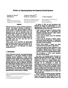
The MCMC Kernel’s computation is performed by an MCMC Controller, Scoring Unit and Graph Sampler Unit, shown in Figure 2.

3.1.1

MCMC Controller

The MCMC Controller Unit (MCU) performs the sample (order) generation as well as deciding whether to keep or discard a sample based on its score. The MCU uses the two dimensional encoding to represent orders as in [5]. In the two dimensional encoding of an order, each row represents a “local order” and encodes the possible parents of the node

AC

P (B=0)

P (B=1)

00

0.8

0.2

01

0.4

0.6

10

0.3

0.7

11

0.9

0.1

A

C

A

B

a D

C

B

D

b A

B

C

D

0 B 1 C 1 D 1

0 0 0 1

0 1 0 1

0 0 0 0

A

c

Figure 1: A Bayesian Network with 4 variables and Binomial CPDs. a: The CPD at node B, which encodes the distribution of B given different states of its parents. b: An order that is compatible with the graph. c: Two dimensional one-hot encoding of the same order.

corresponding to that row, as is shown in Figure 1. The MCU performs the random walk by swapping the position of two nodes (corresponding rows and columns in the two dimensional encoding) to create new samples, and accepts the new sample with probability A based on the MetropolisHastings rule: ! 0 0 Score(≺ |D) A(≺→≺ ) = min 1, Score(≺ |D) Since the scores represent very small probabilities, all computations are done in logarithmic (log) space. This also allows the reduction step on the FPGA to be implemented as simple additions rather than multiplications. Therefore, the MCU decides whether to keep the new sample by subtracting the old score from the new score and compares this number to the log of a random number. A hardware LFSR and a log look-up table are designed to generate the required random numbers.

3.1.2

MCMC Scoring Unit

When the MCU generates an order, the MCMC scoring unit (MSU) is responsible for calculating and returning the resulting score to the MCU. As introduced in Section 2, the scoring process for each local order involves traversing over a set of parent sets (stored in memory) and accumulating the local score of each compatible parent set. The accumulation process is associative and commutative and can be decomposed into as many smaller, parallel accumulations as the implementation platform can accommodate. On Virtex-5 FPGAs, each accumulation circuit (called a scoring core or ‘SC’) requires Block RAM (BRAM) for parent set and local score lookups, regular FPGA logic to implement the accumulator itself, and either BRAM or distributed/LUT RAM (LRAM) to implement a log lookup operation. Score look-ups are made with BRAMs because of their high bandwidth and single cycle access. Using LRAM for log look-ups saves BRAM resources for parent sets and scores but constrains routing high-utilization/frequency designs. At the MSU’s top level, the logic responsible for scoring one node (or ‘SN’) is replicated for each node that the system must support. Nodes are then divided into SCs, which are

Ethernet Node Scores

PLiN

Node

Platform Interconnect Network

PLiN

Node MCMC Controller

RCBIOS Harness

PLiN

Previous Node

Order Score

+ Graph Score

Node

Scoring Datapath

Score Threads

Scoring Data Scoring Logic

One node

Resulting Score Proposed Order

Score

Score

Accumulator

Enable?

Parent Set Local Order

Score Threads

Graph Sampler

Block RAM

Scoring Datapath

Local Order (from MCMC Controller)

Graph Sampler

Enable?

+

Scoring Core

PLiN

Key

Graph Sampler

Scoring Core

MCU

Block RAM Column

Local Order Parent Set

Scoring Core

Next Node

Block RAM Column

RCBIOS Harness

LOG Table

LOG Table

Previous Core Graph Sampler

Scoring Post-Processor

Graph Sampler Accumulator

Scoring Core

Graph Sampler

Xilinx Virtex-5 LX155T FPGA

+

Next Core

Graph Sampler Accumulator

29 node system 3 scoring cores per node

Figure 2: A ParaLearn MCMC Kernel on a single FPGA, supporting 29 nodes. assigned BRAM perSC 18Kbit BRAM, given by: ‰ ı ‰ ı Network Size FP Precision BRAMperSC = + 1 1 32 × Ports 32 × Ports P orts is either 1 or 2 for Virtex-5 FPGA BRAMs, meaning that each BRAM can be dual-ported to increase performance. Within each SC, the score accumulation datapath is pipelined and time-multiplexed between hardware scoring threads in order to maintain a one-score-per-cycle accumulation in the steady state, regardless of clock frequency. Each SN is assigned as many SCs as is necessary to support the problem specified parent-sets-per-node (PPN) constraint. This architecture strives to minimize BRAM depth and maximize throughput per SC, which in turn maximizes performance. When the MCU broadcasts an order, the order is split into local orders and, through a pipeline that fans out across the FPGA, sent to each node’s SCs in parallel. Each SC starts

and finishes scoring its local order at the same time since the scoring process is a data independent memory traversal. Once scoring is complete, each SC’s result is accumulated as shown in Figure 3. Linear accumulation is used to accumulate in nearest-neighbor fashion across SCs and SNs because the Virtex-5 FPGA’s BRAMs are arranged in columns. To avoid rerunning FPGA CAD tools for different networks, each node and SC in the MSU can be enabled or disabled at runtime. Each SC that does not receive any parent sets from software is considered disabled and is bypassed during the score accumulation process. If all SCs within an SN are bypassed in this way, the entire SN is bypassed. This means that an MCMC Kernel that is designed to accommodate an N node and P PPN system can accommodate any number of nodes ≤ N and any number of PPN ≤ P. When the system is synthesized to support more PPN than it needs to support a given network, the system can

tio n

Node i has been enlarged

Internet

In iti al iz a

From RCBIOS / Software Pre-Processing (initialization)

Hardware

Scoring Core

Software

Block RAM

NoC Switch

Port A

+

MCMC Kernel

+

+

+

+

RDMA NoC Switch

Cross-Thread

+

Cross-Port

+

+

Node N

Cross-Core

Lo

ca

Register File

Pre-Processing

RDMA

Parent Sets & Local Scores

Node i+1

NoC Switch

Stream

PostProcessing

Stream

ParaLearn N

UART or Ethernet

Register File

+

Local O rder i

Hardware Threading

er rd lO

NoC Switch

+

+

Port B

RCBIOS

XLink

RCBIOS

ParaLearn Re

Node i

su lts

Internet

Local Order i+1

From Node i-1 +

+

+

MCMC Controller

Figure 3: Abstract connectivity and reduction tree for the MSU. This example shows two threads per port, two ports per SC, three SCs per node, and N nodes. achieve a greater speedup. This is because every parent set BRAM is designed to behave like a restartable FIFO. Thus, each SC only scores as many parent sets as have been loaded at initialization. By spreading out parent sets across the SCs as evenly as possible, the kernel can optimize at runtime for arbitrary problems.

3.1.3

MCMC Graph Sampler Unit

Determining which graph will produce the highest score from each order is a process typically undertaken by software after order sampling is complete [17]. ParaLearn’s FPGA Kernel determines graphs and their scores in parallel with the order scoring process. The highest scoring graph consists of the highest scoring parent set for each node. Thus, each SC must keep track of the highest scoring parent set it has seen throughout each iteration. When order scoring is complete, the graph score is accumulated separately across SCs and the graph itself is assembled and sent to software (see the “Graph-Samplers” in Figure 2). Assembling the final graph takes more clock cycles than accumulating the order score, so the ith order’s graph is assembled while the (i + 1)st order is issued by the MCU. Through integrating the graph sampling step into the order sampler, graph sampling costs zero time overhead.

3.1.4

GateLib & RCBIOS

GateLib [12] is a standard library of hardware and software code with an integrated build and test framework. GateLib was developed at U.C. Berkeley and includes everything from standard registers, to DRAM controllers, to build and test tools which ensure that both the library and designs such as ParaLearn are operating correctly. For ParaLearn the most significant component of GateLib is the sub-library called RCBIOS, which provides a Reconfigurable Cluster Basic Input/Output System for the kind of FPGA computing platforms used in this work. RCBIOS provides three primary interfaces between hardware and software: remote memory access (RDMA), control and status registers and data streams. RCBIOS is built on top of a flexible Network-on-a-Chip interconnect and XLink, another sub-library of GateLib which provides simple hard-

Figure 4: RCBIOS infrastructure and hardware/software blocks supporting MCMC. From right to left, the system is initialized. From left to right, results are collected. ware/software communication. Implemented directly in RTL Verilog (i.e. without any service processors), the RCBIOS modules provide high-performance, low cost and easy-to-use communications between the FPGAs and the front-end system. ParaLearn uses RCBIOS to initialize system state and to collect resulting graphs and their scores as shown in Figure 4. After the pre-processing step, ParaLearn software uses RCBIOS to send parent sets, local scores, a node count, an iteration count, and an initial order to the reconfigurable cluster (referred to as Load T ime). As each order is scored, its highest scoring graph and that graph’s score is streamed back to software and post-processed.

4.

SCALABILITY

When the problem becomes too large for a single FPGA, the MCMC Kernel must be spread across multiple FPGAs. ParaLearn leverages the BEE3 [2] platform’s mesh network (see Figure 5), composed of both interchip links between the four FPGAs, and CX4 links between BEE3’s. A multiFPGA MCMC Kernel is composed of a master FPGA and one or more slave FPGAs. The master FPGA contains MCU and MSU logic. The slave FPGAs are used for their MSUs only and score any local order which arrives, returning the partial score to the master FPGA. In all cases, since the logic which differentiates master and slave is relatively small compared to total FPGA area, a single FPGA bit-file is used for both master and slave, and each is configured at runtime through software. This simplifies the process of reconfiguring and managing the system as more FPGAs need to be introduced to support larger problems. ParaLearn augments the BEE3 mesh network with a general cross-chip router to support additional FPGAs without having to modify the pre-existing system. The router, a dedicated circuit called the “Platform Interconnect Network” or PIN [18], interfaces with firmware designed to support both interchip tuning and interboard protocols. Furthermore, PIN uses dimension order routing to channel packets both to and from the master FPGA. When the MCU broadcasts an order, a subset of the order is sent directly to the master’s MSU, and the remainder is packetized and sent to the slave FPGAs in the system. As the scoring process takes

BEE3

D

C

B

A

C

D

B

A

BEE3 D

C

BEE3

BEE3

B

A

Key Master FPGA Slave FPGA

B

A

BEE3

B

A C

Proposed Order Resulting Score

D

C

BEE3 D

BEE3

BEE3 Rack (Reality)

BEE3 Rack (Physical Connections)

BEE3

BEE3 Rack (Flattened View & Logical Design Routing)

Figure 5: Different views of a multi-FPGA ParaLearn Kernel. the same amount of time for every node, the master FPGA decreases total scoring time by sending local orders to slave FPGAs whose hop latency to the master1 is greatest, first. The hop latency is made up of hops across interchip and interboard links, and therefore is not completely determined by the manhattan distance between two FPGAs.

4.1

FPGA Platforms

ParaLearn’s scalability, coupled with the dearth of industry standards, makes it important for us to address the tradeoffs between different multi-FPGA or reconfigurable cluster platforms. Reconfigurable cluster platforms differ in the number and type of FPGAs per board, the connection topology, as well as supported peripherals and interfaces. Platforms range from the Dini Group DN9000K10 which consists of a mesh of FPGAs, to the Xilinx ACP that uses an Intel front-side-bus (FSB) to connect a smaller number of FPGAs to a CPU. ParaLearn targets the BEE3 reconfigurable cluster platform from BEEcube [2]. The BEE3 consists of four Virtex5 LX155T FPGAs, two channels of DDR2 SDRAM perFPGA, and a point-to-point interconnect. The interconnect for each FPGA consists of two “interchip” links, which form a ring on the board, and two 10GBase-CX4 Ethernet interfaces for interboard connections. ParaLearn as discussed in section 4, uses these connections to assemble a mesh network of MCMC cores. Unlike platforms that embed a full network of FPGAs in a single PCB, such as Dini Group boards, the CX4 connections on the BEE3 are cable-based, which allows the system to be reconfigured to meet the application’s needs. This allows different FPGAs in the system to be connected directly together in order to reduce inter-FPGA hop count, or to increase the size of the overall system. These CX4 connections come at a price, having latency on the order of several dozen cycles, as opposed to the 5 cycles between FPGAs on one board. When comparing the BEE3 against bus-connected platforms like the Xilinx ACP, there is a tradeoff between cluster size and front-end communication. Bus-connected platforms like the ACP are limited by bus sharing and score accumu1

Measured in clock cycles across the mesh.

lation will scale linearly in time with the number of FPGAs. By contrast the BEE3 can take advantage of score reductions at each hop, accumulating multiple FPGA’s score at a single time. Furthermore, the cost of the ACP systems must include a processor which is of no particular use to ParaLearn and adds to purchase, complexity and maintenance costs. While ParaLearn is currently implemented on a BEE3 system due to the characteristics of the algorithm, this is not the only compatible implementation platform, and the system can be efficiently implemented on other platforms. In particular the system was developed in part on the Xilinx ML505 demonstration boards, which are comparable to a quarter of a BEE3, and provide a low-cost entry level FPGA platform.

5.

RESULTS AND ANALYSIS

Our primary study analyzes 22 proteins in human cancer T-Cells with data from CyTof technology. We use 10,000 single cell measurements of the 22 proteins and limit the search indegree for the graph search to 4. Therefore, we have 7547 possible parent sets for each node and that we need at least two Virtex-5 LX155T FPGAs to implement one MCMC Kernel.

5.1

Quality of Results

To assess the correctness of the FPGA design, we tested the software and FPGA versions of the algorithms on synthetic data simulated from known BN structures such as the ALARM [1] network and we were able to reconstruct the network on both implementations. The only approximation in the FPGA implementation compared to the software version is the fixed point conversion of the local scores and lookup table entries. We used 32 bit fixed-point precision and while this results in a small change in the graph scores (less than 0.1 - that is about 0.1% of the score), the relative orderings of the graph structures do not change and the best graph structures found by the two implementations are identical. With simulated data like the ALARM network, the CPD formulations are known, while with real data like CyTof, we do not know which CPD is the closest representative of the underlying interactions in the system. Therefore we applied two different CPD formulations to learn the interaction in this system—shown in Sections 5.1.1 and 5.1.2.

As we expected the final results of the two kernels are significantly different. The Multinomial encoding results in a sparser model with 14 edges while the Linear Gaussian results in a denser model with 63 edges. There are 6 edges that appear in both models. These different graphs need to be further validated by scientists and domain experts and their true quality should be measured by their predictive power on new data sets from the STN.

5.1.1

Multinomial CPD

For the Multinomial representation we need to discritize raw data that is continuous. We used Biolearn software [3] to perform the discritization to a three-level discrete data set. The local score of a given parent set for each node using Bayesian formulation (with Dirichelet priors on parameters) is calculated as: BayesianLocalScore(Vi , Πi ; D) ! |Vi | ri Y Y Γ(Nijk + αijk ) Γ(αik ) LSVi ,Πi = log Γ(αik + Nik ) j=1 Γ(αijk ) k=1 Q where ri = Vj ∈Πi |Vj | [7]. α is the BDe prior parameter introduced in [14]. Nik and Nijk are sufficient statistics (counts) that are calculated from experimental data D.

5.1.2

Linear Gaussian CPD

The joint probability distribution of variables in a Gaussian network is a multivariate Gaussian distribution. We used the BIC scoring method and, as shown in [11], the local scores can be calculated as: BICLocalScore(Vi , Πi ; D) LSVi ,Πi

m X −mn = log(2πe) − n log 2 i=1

detS πi X detS πi

!

that describe how many SCs should be instantiated in each node, and also how each of the SCs should be implemented. To build the optimal configuration, the software generator first determines the theoretical maximum performance through fixing the network size, PPN, and hardware resources, while scaling the number of SCs per node. Generally, performance will increase with the number of SCs to the point where the result accumulation step overwhelms the SC’s execution time. Figures 7 and 9 exemplify the pare-to optimum curves as a function of SCs per node. The generator varies the number of SCs per node by adding more single-ported SCs or dual-porting existing SCs. Adding single-ported SCs costs the most BRAM and FPGA logic, but can be done incrementally until the system runs out of FPGA fabric. Using dual-ported SCs is “all or nothing”—if one SC is dual-ported, the rest have to be as well or the performance benefit is masked by the slower SCs. Adding single-ported SCs also increases the maximum PPN that the system can support, while dual-porting does not. ParaLearn dual-ports SCs when the required PPN is low or the system is BRAM constrained.

5.2.2

In this section we compare the 22 parameter2 CyTof data across currently attainable3 FPGA configurations in order to show how speedup and power consumption is affected by the hardware configuration used to support the problem. BRAM port mode

log(n) X |Πi | −γ 2 i

Single

where m is the number of variables and n is the number of observations. S πi X is the covariance matrix of the node and its parents and S πi is the covariance matrix of the parent variables. γ is the penalty parameter that is used to adjust the BIC score to penalize the more complex networks in the search algorithm.

5.2

Single Double

Design Space Exploration

Single

Sections 5.2.2 through 5.2.5 present different studies used to evaluate ParaLearn in terms of scalability, performance, area and power. In our analysis, we use an “orders per second” (OPS) metric to determine performance. Unless otherwise noted, all tests are run on the following hardware:

Double

FPGA: Xilinx Virtex-5 XC5VLX155T (-2 speed) FPGAs

Single

GPP: Intel(R) Core(TM) i7 CPU QuadCore running at 3.07 GHz, with 12 GB of Memory and with an advertised TDP of 130 W. For perspective, the Virtex-5 is a generation-old FPGA family and the XC5VLX155T is a mid-sized chip in the family.

5.2.1

Software Generator

To help conduct performance studies, we use software to generate MCMC Kernels that are optimized for different networks. The generator takes as input the desired network size, PPN, and parameters describing the implementation platform (such as BRAM dimensions and the number of FPGAs available to solve the problem). From this information, the generator sets parameters used by the FPGA CAD tools

Current Scalability

Double

SCs / FPGA

Clock (Mhz)

OPS

Power / FPGA (W) Two FPGAs (nodes per FPGA = 11) 88 100 86,730 10.56 150 122,951 13.82 Three FPGAs (nodes per FPGA = 8) 64 100 88,106 10.33 150 124,792 12.38 200 159,109 10.96 128 100 144,092 11.72 150 195,567 14.39 Four FPGAs (nodes per FPGA = 6) 48 100 84,962 9.94 150 119,048 11.26 200 153,022 10.13 96 100 137,363 10.56 150 184,729 12.80 200 226,501⊕ 11.85 Eight FPGAs (nodes per FPGA = 3) 24 100 77,640 9.73 150 109,649 11.06 200 152,091 10.33 48 100 114,679 10.68 150 160,600 11.06 200 201,005 10.51

Power / Problem (W) 21.12 27.64 30.99 37.14 32.88 35.16 43.17 39.76 45.04 40.52 42.24 51.20 47.40 77.84 88.48 82.64 85.44 88.48 84.08

Table 1: MCMC Kernel study on the 22 parameter CyTof data (P P N = 7547) on one and two BEE3 boards. The highest performance “attainable” configuration for each system composed of N FPGAs is shown in bold. The OPS column in Table 1 shows the performance impact of spreading the 22 parameter problem across different 2

One parameter corresponds to one node. An “attainable” configuration can fit into the allotted hardware and meet timing at the specified frequency. 3

5.2.3

Projected Scalability

In this section, we explore how larger FPGAs can be used to increase system speedup. For this experiment, we used the software generator (Section 5.2.1) to project performance over a range of SC counts per node (shown in Figure 7). We verified these trends through: 1. Direct comparison with hardware performance for “attainable” configurations. 2. Gate-level simulation at fixed intervals on the curve, and at the projected upper-bound, for configurations requiring larger FPGAs. Extrapolated from Figure 7, larger FPGAs will provide between 1.5× and 1.7× speedup over current configurations assuming a comparison across the same number of FPGAs. If the problem is able to fit onto a single FPGA, power will be minimized4 and speedup can increase by up to 2.61×. 4 In addition to saving power with less FPGAs, single FPGA configurations do not use interchip and GTP connections, which we showed to be a large contributor to total power consumption.

700000

1 FPGA 2 FPGAs

600000

3 FPGAs

OPS

500000

4 FPGAs 8 FPGAs

400000 300000 200000 100000 0 1

11

21

31

41

51

61

71

81

91

Scoring Cores per Node

Figure 7: Scaling the number of SCs per node for the 22 parameter CyTof data. All experiments are carried out with dual-ported SC BRAMs, a 200 Mhz clock, and assuming that an FPGA chip can support any number of SCs. The vertical bar indicates the point that our current hardware allows us to achieve. 400000 350000 300000 250000

OPS

arrangements of FPGAs. For each number of FPGAs, trials are run for {100, 150, 200} Mhz clock frequencies and for both single and dual-ported SCs. To isolate the effect of scaling across FPGAs, all configurations support exactly 8 single or dual-ported SCs per node. If a configuration in this permutation isn’t listed in Table 1, it was not attainable. As more FPGAs are used to support the problem, configurations using the same number of SC ports and the same clock frequency tend to degrade in performance due to an increased hop latency in the FPGA mesh. With additional hardware, however, more aggressive configurations (in terms of SC porting and clock frequency) become “attainable.” The Power columns in Table 1 show power utilization for different configurations. All power results are gathered through the Xilinx XPower Analyzer after simulating traces through the system running the 22 parameter CyTof data set. As we have fixed the number of SCs per node in each experiment, the power consumption per FPGA drops in sparser FPGA configurations however total system power (taking into account the number of FPGAs) tends to increase. We found that this is due to fixed cross-FPGA communication overhead, namely the interchip links in each sample (which produced ≈ 3.8 W ) and the GTP connections (responsible for ≈ 1 W ) in the 8 FPGA experiment. Furthermore, Table 1 shows that in general, 150 Mhz configurations require more power than 200 Mhz configurations. We attribute this to there being an extra clock in 150 Mhz configurations (interchip requires a 200 Mhz clock and RCBIOS requires a 100 Mhz clock—thus the MCMC Kernel can use those existing clocks when running at 100 or 200 Mhz). Figure 6 shows the FPGA resource utilization for all attainable 2–4 FPGA configurations in Table 1. In general, using dual-ported SCs increases performance improves by ≈ 1.6× and more evenly uses FPGA resources. In practice, we observed that designs that utilize a majority of FPGA logic resources could not route at higher frequencies when LRAM was also heavily utilized. To get around this problem for 200 MHz configurations, we more heavily relied on BRAM rather than LRAM to implement log tables, relative to 150 MHz configurations.

200000 150000 100000 50000 0 1

11

21

31

41

51

61

71

81

# FPGAs

Figure 8: Scaling the number of FPGAs for the 22 parameter CyTof data. Samples are taken at 200 Mhz with dual-ported SCs. It is also important to consider how performance degrades as the number of FPGAs in the system increases. To isolate this effect, we constrain the software generator to 8 dual-ported SCs per node while increasing the number of FPGAs, as shown in Figure 8. In order to maximize performance, each FPGA mesh is arranged so that the hop latency from the master FPGA to any given slave FPGA is minimized. The occasional kinks in the graph are due to adding an FPGA with a new greatest hop latency. As can be seen, the greatest performance hit is moving from one to two FPGAs, with the performance decreasing linearly as the number of FPGAs increases.

5.2.4

Current Flexibility

This section studies how ParaLearn can scale to handle different networks. As the FPGA CAD tools take an appreciable amount of time to run, it is important to study how a general FPGA bitfile, configured for up to N nodes and P PPN performs

100 90

% Utilization

80 70

SP,100

60

SP,150

50

SP,200

40

DP,100

30

DP,150

20

DP,200

10 0

FF

SLICE LUT(T) LUT(L) LUT(M) BRAM

FF

2 FPGAs


3 FPGAs

FF


4 FPGAs

Figure 6: Resource utilization for the 22 parameter CyTof data. “LUT ({T, L, M})” refers to total LUTs, LUTs used as logic, and LUTs used as memory (LRAM), respectively. Each dataset is labeled “{S,D}P,X” which refers to single or dual-ported SC schemes and the clock frequency (‘X’) in Mhz. for different problems. Table 2 shows different configurations for problems spanning over four FPGAs (a single BEE3 board). All configurations maximize PPN and place performance as a second-order constraint in order to tolerate denser networks. Thus, this study synthesizes only singleported BRAMs and shows results for the highest attainable clock frequency (150 MHz for every experiment). All configurations are first shown assuming that all available parent set memory is used. The 22 parameter CyTof data’s performance is shown in rows whose PPN column is marked with a ?. The closest configuration to the CyTof data (A ) achieves .8× performance relative to the most aggressive, attainable bitfile (marked ⊕ in Table 1) while the next closest (B ) achieves .6× the performance, and the last (C ) maintains .4× performance. The drop-off is due to there being less SCs per FPGA, which is due to larger networks requiring wider parent set logic. Nodes

Nodes /

SCs /

FPGA

Node

8 16 24

2 4 6

58 28 15

Max 59,392 28,672 15,360

32

8

11

11,264

40

10

8

8,192

PPN Actual 128 28,672 15,360 ?7,547 11,264 ?7,547 8,192 ?7,547

OPS Limited 99 1,941 10,903 “” 4,992 “” 9,920 “”

− 113,208 110,457 180,288A 103,306 134,168B 91,296 94,399C

Table 2: MCMC Kernel flexibility study. All experiments are carried out with single-ported SCs and a 150 Mhz clock. “Max” refers to the highest PPN that our current hardware can support, “Actual” corresponds to the PPN used to benchmark the system (performance is shown in the “OPS” column) and “Limited” is the PPN when the indegree is fixed (Section 5.2.5). Table 2 also shows the point at which the MCMC Kernel becomes BRAM limited in handling different networks. For a network of N nodes, there are a possible 2N −1 different parent sets. Theoretically, the 8 node network across four FPGAs can tolerate 59,392 parent sets but a network of that size will only ever have 28−1 = 128 parents (for this reason,

an 8 node network would never be spread across four FPGAs in practice). The 16 node network, on the other hand could have 32,768 different parent sets, yet the MCMC Kernel can only tolerate 28,672 parents. ParaLearn tolerates BRAM constrained networks through limiting the number of parent sets. This can be done in two ways: 1. Using smarter parent set filtering algorithms based on supervised learning techniques that can learn the subset of variables that are correlated with a node value and then include those as possible parent sets. 2. Limiting the maximum indegree of the graphs. With this approach, ParaLearn includes parent sets up to size K, where usually 2 < K