Parallel Hybrid Clustering using Genetic Programming and Multi ...

Parallel Hybrid Clustering using Genetic Programming and Multi-Objective Fitness with Density (PYRAMID) Samir Tout 1 , William Sverdlik 2 , Junping Sun1 Abstract—Clustering is the process of locating patterns in large data sets. It is an active research area that provides value to scientific as well as business applications. Practical clustering faces several challenges including: identifying clusters of arbitrary shapes, sensitivity to the order of input, dynamic determination of the number of clusters, outlier handling, processing speed of massive data sets, handling higher dimensions, and dependence on user-supplied parameters. Many studies have addressed one or more of these challenges. This study proposes an algorithm called parallel hybrid clustering using genetic programming and multi-objective fitness with density (PYRAMID). While still leaving significant challenges unresolved, such as handling higher dimensions and dependence on user-supplied parameters, PYRAMID employs a combination of data parallelism, a form of genetic programming, and a multiobjective density-based fitness function in the context of clustering to resolve most of the above challenges. Preliminary experiments have yielded promising results. Keywords: Data Mining, Clustering, Genetic Programming, Parallelism, Density. I. INTRODUCTION

C

LUSTERING is a technique used to unravel data distributions and patterns in a data set by means of a supervised [3] or unsupervised [6] classification of those patterns. Example clustering applications include multimedia analysis and retrieval [7], pattern recognition [10], and bioinformatics [3]. Considerable research continues in the field of clustering, involving numerous disciplines. This opens avenues for further research and introduces new challenges that become core issues to be tackled by clustering algorithms. These include: accommodating arbitrary-shaped (non-rectangular) clusters, sensitivity to the order of input, dynamic determination of the number of clusters, handling outliers, processing speed of massive data sets, handling higher dimensions, and dependence on user-supplied parameters. This paper proposes an algorithm called Parallel hYbrid clusteRing using genetic progrAmming and Multi-objective fItness with Density (PYRAMID). While still leaving significant challenges unresolved, such as handling higher dimensions and dependence on user-supplied parameters, PYRAMID employs a 1 2

combination of data parallelism, genetic programming (GP), special operators, and multi-objective densitybased fitness function in the context of clustering to resolve most of the above challenges. The data space is divided into cells that become the target of clustering thus eliminating dependence on the order of data input. A divide-and-conquer data parallelism is used to achieve speedup. The algorithm divides the data set onto multiple processors each of which executes a genetic program that uses a flexible individual representation that can represent arbitrary shaped clusters. The genetic program also utilizes a densitybased fitness function that helps avoid outliers. It also introduces a merge method that determines the number of clusters dynamically. Preliminary experiments have shown positive results. The rest of this paper is organized as follows: Section 2 enumerates some related work. Section 3 defines key concepts that play an essential role in this study. Section 4 elaborates on the PYRAMID approach. Section 5 provides details about the experiments and their results. Finally, Section 6 states the conclusion of this research and future directions. II. RELATED WORK

A plethora of valuable algorithms were developed to tackle some of the above mentioned issues, but each of those concentrated on a specific aspect. For instance, BIRCH [18] focused on speed by means of data summarization but favored circular clusters [9]. CURE [5] concentrated on sampling and outlier handling. DBSCAN [4] yielded good detections by favoring dense neighborhoods. As reported in [8], CURE and DBSCAN did not always detect outliers and depended on user-supplied parameters. RBCGA [12] used a genetic algorithm that utilized rectangular shapes, called rules, each representing a cluster, thus only accommodating rectangular cluster shapes. NOCEA [13] improved over RBCGA by providing multiple rules per cluster, thus offering better detection than RBCGA but, as stated in [13], its crossover operator broke large rules and did not always detect sparse areas within those rules, thus resulting in coarse detections.

Graduate School of Computer and Information Sciences, Nova Southeastern University, Fort Lauderdale, FL, 33314 Department of Computer Science, Eastern Michigan University, Ypsilanti, MI, 48197

III. DEFINITIONS This section introduces terms and concepts that are pertinent to the PYRAMID algorithm. In all definitions, n symbolizes the number of points in a data set and d is the number of dimensions. Definition 3.1: A Minimum Bounding HyperRectangle (MBHR) is the smallest hyper-rectangular area in the data space that contains all the ddimensional data points in a given data set [11]. In a two-dimensional space, a minimum bounding hyperrectangle is simply denoted minimum bounding rectangle (MBR). Definition 3.2: Binning of dimension m within the MBHR where m = 1, …, d, is the division of the maxis into tm non-overlapping segments, called bins. This study adopts a binning approach that is similar to the one used in NOCEA, which relies on a theoretical foundation presented in [14]. All bins within a dimension m have the same bin width, denoted wm. This is calculated according to (1), where σm is the standard deviation of the coordinates of the data points on dimension m. (1) w m = 3 .5 × σ m × n −1 / 3 There is no overlap between any two bins within the same dimension. The lower and upper bounds of the ith bin with respect to dimension m, called bini,m, are respectively denoted lb_bini,m and ub_bini,m Definition 3.3: After binning is performed on every dimension m where m = 1, …, d, the intersections of the bin lines construct a d-dimensional grid that divides the MBHR into contiguous non-overlapping ddimensional cells, denoted quantization. A cell c has a corresponding bin with respect to every dimension m, which is the projection of c onto m. Cells inherit the property that no two cells overlap. Furthermore, cells have the following property: ∀ cell c, width of c with respect to dimension m = wm. Definition 3.4: Volume of a cell c, denoted vol_cell(c) is the product of c’s widths with respect to all dimensions. This is given by (2). Since all bins have the same width with respect to a certain dimension, the volumes of all cells are equal. d (2) vol_cell ( c ) = ∏ m = 1 w m Definition 3.5: Cardinality of a cell c, denoted card_cell(c), is the number of data points that fall within the bounds of c. Definition 3.6: Density of a cell c, denoted as dens_cell(c), is the ratio of the cardinality of c over its volume. This is demonstrated in (3). card_cell ( c ) (3) dens_cell ( c ) = vol_cell ( c )

Dense cells are desirable candidates to be part of a good clustering solution. Definition 3.7: Rule r is the hyper-rectangular subregion of the MBHR that contains one or more cells. Those cells are denoted constituent cells of r. A rule has a lower and an upper bound with respect to every dimension, represented as follows: rule(lb_rule1:ub_rule1, ..., lb_ruled:ub_ruled) where lb_rulem and ub_rulem, m = 1, ..., d, are calculated respectively as the minimum lower bound and maximum upper bound of all its constituent cells with respect to dimension m. A rule r is said to overlap with another rule r’ if they share at least one common constituent cell. This study does not allow overlapping rules within the same solution. Definition 3.8: Volume of a rule r, denoted vol_rule(r) is the sum of the volumes of its constituent cells. Definition 3.9: Cardinality of a rule r, denoted card_rule(r), is the number of data points that fall in r’s constituent cells Definition 3.10: Density of a rule r, denoted dens_rule(r), is the ratio of the cardinality of r over its volume. This is demonstrated in (4). card_rule ( r ) (4) dens_rule ( r ) = vol_rule ( r ) Dense rules are desirable candidates for good solutions. Definition 3.11: Individual I is the region in the MBHR that is a union of rules, called I’s constituent rules. In the context of clustering, an individual constitutes one possible solution to the clustering problem at hand. A list of the constituent rules of an individual I and their constituent cells, commaseparated, is called the individual profile, or profile(I). Definition 3.12: Volume of an individual I, denoted vol_indiv(I) is the sum of the volumes of its constituent rules. Definition 3.13: Cardinality of an individual I, denoted card_indiv(I), is the sum of the cardinalities of I’s constituent rules. An individual contains no overlapping since its constituent rules; based on Definition 3.7, do not overlap. Definition 3.14: Density of an individual I, denoted dens_indiv(I), is the ratio of the cardinality of I over its volume. This is demonstrated in (5). card_indiv ( I ) (5) dens_indiv ( I ) = vol_indiv ( I ) It is worth noting that individuals with higher density constitute good candidates for clustering solutions. Definition 3.15: Size of an individual I, size(I), is defined as the number of constituent rules in I.

Definition 3.16 Speedup measures the ratio of the serial processing over the parallel processing using those p processors. It is defined as: speedup =

Serial − execution − time − on − 1 − workstatio n Parallel − execution − time − on − p − worksation s

(6)

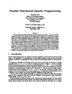
Definition 3.17 The i-th Column, with respect to dimension m, denoted coli,m, in a quantized MBHR, is the set of cells that have the same corresponding i-th bin, with respect to dimension m, i.e., bini,m. In a twodimensional setting, the columns with respect to the yaxis are denoted rows. Definition 3.18 Geometric Division is an algorithm that divides the data space into quadrants. A quadrant encompasses a data subset, which is formed by the data points that belong to its constituent cells. The details of this algorithm are outlined in Fig. 1.a while Fig. 1.b displays a sample geometric division on a twodimensional data set. Fig. 1.b. Quantization and geometric division. 1. Select v, number of divisions per dimension. Calculate required division subset size as s = n/v, where n is the number of points. 2. For every dimension m = 1,...,d, traverse grid columns from lower to upper bin numbers, adding the cardinalities of their constituent cells. Stop when > s. 3. Compare which is closest to s: before or after adding the last column. If before, do not count the last column, else count it. 4. Continue until v divisions have been identified. 5. The intersections of the resulting divisions on every dimension form the p = vd subsets, called quadrants, which will be transmitted to the p slave processors 6. Examine number of data points in every quadrant. If one quadrant contains less than half of an adjacent quadrant, adjust border between the two quadrants, with respect to all dimensions if necessary, until that is not the case anymore. Repeat for all quadrants. Fig. 1.a. Geometric division algorithm.

IV. THE APPROACH PYRAMID is a multi-step hybrid approach that is based on several components that utilize the above concepts. For the sake of simplicity, the rest of this study focuses on two-dimensional data sets as in [8] and leaves higher dimensions for future research. The PYRAMID algorithm is summarized in Fig. 2. A. Data Transfer from Master to Slaves As mentioned earlier, the geometric division algorithm forms quadrants as groups of cells. The master processor sends each quadrant’s data subset to a separate slave processor where another quantization is performed and a genetic program is executed.

Master Processor 1. Conduct binning on MBR. 2. Perform geometric division. 3. Send each subset to a different slave processor. 4. Receive p resulting subsets of discovered data points from p slaves. Determine cells that contain returned points. Mark those cells as returned cells. 5. Merge returned cells into global solution that labels every cell with a cluster label. Slave Processor 1. Receive a data subset P from master processor. Perform quantization on local data. 2. Run genetic program on the local data points in P (on current slave processor). 3. After algorithm finishes, send points in discovered cells to master processor. Fig. 2. Master and slave roles in PYRAMID.

B. Genetic Program A genetic program typically represents a solution as a tree-based individual [10]. In this study, each individual is encoded as a combination of blocks (rules) to form a genetic programming tree with leaf nodes symbolizing these constituent rules. This representation offers more flexibility than genetic algorithm-based bit-strings [10]. A sample is shown in Fig. 3, which demonstrates the tree representation for individual I1 from Fig. 4. As in standard genetic programming, the internal nodes represent the functions that apply to the leaf nodes [10]. In this study, the only function employed is union, which symbolizes that the individual is formed as a combination of its constituent rules (leaf nodes).

Fig. 3. Individual I1 tree representation.

Fig. 6. Enlarge and shrink mutation operators.

Fig. 7. Add and delete structural operator. Fig. 4. Rules for individual in Fig. 3.

1) Genetic Operators Crossover: PYRAMID conducts rule-level crossover by swapping rules between individuals thus producing two new individuals. This is shown in Fig. 5.

Fig. 5. Crossover operator.

Smart Mutation: PYRAMID examines the densities of the cells that surround the target rule and performs enlarge mutation towards the denser cells. Another variant of mutation is shrinking whereby a rule is diminished by one bin with respect to a certain dimension m. Mutation always produces one new individual, as shown in Fig. 6.

Architecture Altering (Structural): This operator permits PYRAMID to add a new rule or delete an existing one as demonstrated in Fig. 7. Repair Operator: Overlaps occur when one of the above operators produces a change in an existing rule, or an addition of a new rule, that shares at least one cell with an existing rule within the same individual. As mentioned earlier, overlaps are prohibited by PYRAMID. Therefore, this study introduces a novel repair operator that results in smoother detection by reforming the overlapping rules into new ones that align better with the distribution of the data points. The repair algorithm is shown in Fig. 8 and exemplified in Fig. 9 where the outside frame depicts the area covered by the original overlapping rule. 2) Fitness Function This study focuses on three main factors to achieve good solutions. It attempts to find a solution that captures as much of the data set as possible, thus high coverage. It also tries to identify gatherings of dense areas in the MBHR by looking for solutions in the form of dense individuals composed of dense rules that contain dense cells. Finally, it attempts to avoid complex individuals by having a bias in favor of those having a smaller number of member rules. Therefore, based on the above three factors, this research attempts

to identify better solutions, or individuals, by incorporating, in its fitness function, the following three main objectives, leading to (7). 1. Maximize Fcoverage(I) which is the number of data points in an individual over the total number of data points [13]. 2. Maximize Fdensity(I), which is product of the individual, rule, and cell densities. 3. Minimize Fsize(I), which is the size of the individual by exerting parsimony pressure on large individuals [8]. Fitness ( I ) =

Fcoverage ( I ) × Fdensity ( I )

neighborhoods. This is driven by the algorithm, in Fig. 11, resulting in the final solution.

(7)

Fsize ( I )

1. Calculate average density, Densavg, of all rule member cells. Consider dense cells as those with density greater than Densavg/2. 2. Label the top left cell with 1 if it is dense, otherwise, examine cells to its right until a dense one is found and label it. 3. Traverse rule member cells from top-tobottom, left-to-right. For every dense cell: If top cell dense If left cell not dense, If top left labeled same as top Label with a new label Else set same label as top Else (i.e., if left cell dense) Label same as left Else (i.e., if top cell not dense) If in first row If left labeled Label same as left Else assign new label Else (if not in first row) If left and top left same label Assign new label Else if left labeled Label same as left Else assign new label 4. Form rules from cells with same labels. Fig. 8. PYRAMID repair operator algorithm.

3) Selection Operator and Elitism The selection operator is based on tournament selection with a tour size of three [2]. Furthermore, this study adopts one-individual elitism, whereby in every iteration, the best performer is preserved for the next generation [1]. 4) Main Algorithm The GP that is run on each slave processor is summarized in Fig. 10. After each operator is applied, the fitness of resulting individuals is evaluated. C. The Merge Phase After the discovered points are reported back to the master, which traverses those discovered cells; assigning them cluster labels based on their

Fig. 9. PYRAMID repair operator. t = 0 Initialize population t Evaluate population t While (not termination condition) Begin t = t + 1 s = selection from population t-1 c = crossover 2 individuals in t m = smart mutation a = architecture-altering e = elitism Evaluate(fitness) population t End Fig. 10. Serial GP algorithm. 1. Determine the cells that contain the returned data points, denoted the returned cells. 2. Label all returned cells with “No Label”. 3. Traverse returned cells. For each cell check neighbor cells, as follows: If neighbor cell does not belong to returned cells, skip to the next neighbor, unless that cell is denser than the average density of returned cells, in which case both that and the current cell are assigned same label. Else if neighbor cell is labeled with L1, assign current cell with the same label as neighbor, unless the current cell is labeled with a different label L2, then change both labels to L3. Else if all neighbors are labeled with “No Label”, then assign the current label. 4. Return to Step 3 until all returned cells are processed. 5. Assign different clusters to different labels. Fig. 11. PYRAMID merge algorithm.

V. EXPERIMENTS Several experiments were performed to test the ability of PYRAMID to identify clusters of arbitrary shapes, dynamic determination of the number of clusters, speedup using parallelism, independence of the order of input, and outlier handling. For these experiments, PYRAMID was run over existing twodimensional data sets that were used by other algorithms such as NOCEA, CURE, DBSCAN, and RBCGA. Table 1 shows a list of those data sets. TABLE 1. DATA SETS USED IN PYRAMID EXPERIMENTS. Data Sets Data Objects Clusters DS1 8,000 6 DS2 10,000 9 DS3 100,000 6 DS4 1,120 3

Fig. 12 demonstrates the results that were produced after running PYRAMID on the first three data sets while Fig. 13 shows their detection by NOCEA. Fig. 14 depicts the detection of DS1 and DS2 by CURE and that of DS3 by DBSCAN. The left side of Fig. 15 shows how PYRAMID detected DS4 while the right side shows how RBCGA detected the same. It is noteworthy from Fig. 12 how PYRAMID identified the correct number of clusters. With respect to the goodness of detection, it is evident in Fig. 15 and from a comparison between Fig. 12 and Fig. 13 that PYRAMID provided a smoother detection than RBCGA and NOCEA, respectively. Furthermore, Fig. 12 and Fig. 14 demonstrate how PYRAMID overcame outliers while CURE and DBSCAN did not [8].

Fig. 15. DS4 by PYRAMID versus RBCGA [12].

Concerning the dependence on the order of input, the left part of Fig. 16 shows the result of running PYRAMID on DS1 with its original. The right part depicts the detection after DS1 was shuffled in a completely different order. It is obvious that both detections are fairly similar, thus demonstrating the independence of PYRAMID on the order of input.

Fig. 16. Detection with different data order.

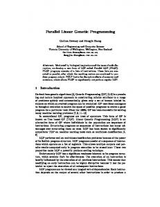
In terms of speedup, Fig. 17 shows the graphs that depict the improvements in speed that PYRAMID achieved from serial to parallel with four processors and sixteen slave processors, for data sets DS1, DS2, and DS3. Table 2 elicits the corresponding speedup values. It is evident that good speedup was attained through parallelism.

Fig. 17. PYRAMID processing speed (seconds) for DS1, DS2, DS3. Fig. 12. PYRAMID cluster discovery.

TABLE 2. SPEEDUP FOR DS1, DS2, DS3. Data Sets Parallel-4 Parallel-16 DS1 1.80 2.84 DS2 2.01 2.86 DS3 2.78 6.43

VI. CONCLUSION AND FUTURE WORK Fig. 13. NOCEA cluster discovery [13].

Fig. 14. Discovery of DS1, DS2 by CURE, DS3 by DBSCAN [8].

This paper proposed a novel approach to clustering large data sets called PYRAMID, which leverages some of the concepts used in NOCEA [7]. However, it improves over that approach by employing a hybrid combination of GP’s global search and strong representational capabilities along with a powerful density-aware multi-objective fitness function. Data parallelism is also employed to achieve speedup. Preliminary results demonstrated that PYRAMID detects clusters of arbitrary shapes, is immune to

outliers, and independent of the order of input. In addition, it does not require prior knowledge of the number of clusters, and its inherent data parallelism allows it to have better performance than its sequential counterpart. One possible avenue for future research is to revisit the PYRAMID algorithm and explore the performance measurements through speedup with higher dimensions. Other avenues include: performing additional experiments to assess various aspects of cluster detection such as the dependence on usersupplied parameters, exploring the use of rules with variable shapes, not strictly rectangular, and using various data sets as well as other forms of parallelism VII. ACKNOWLEDGEMENTS We would like to thank Nova Southeastern University and Eastern Michigan University for providing considerable support for this research. We also extend our gratitude to Keane, Inc. for providing financial support for a portion of this research. VIII. REFERENCES [1] Berkhin, P. (2002). Survey of clustering data mining techniques. Accrue Software. Retrieved February 28, 2005 from http://www.ee.ucr.edu/~barth/EE242/clustering_survey.pdf [2] Davis, L. (1991). Handbook of Genetic Algorithms. New York, NY: Van Nostrand Reinhold. [3] Dettling, M. & Bühlmann, P. (2002). Supervised clustering of genes. Genome Biology, 3(12), 39-50. [4] Ester, M., Kriegel, H.P., Sander, J., & Xu, X. (1996). A densitybased algorithm for discovering clusters in large spatial databases with noise. Proceedings of the Second International Conference on Knowledge Discovery and Data Mining, Portland, Oregon, 226-231. [5] Guha, S., Rastogi, R., & Shim, K. (1998). CURE: An efficient clustering algorithm for large databases. Proceedings of the 1998 ACM SIGMOD International Conference on Management of Data, Seattle, WA, 73-84. [6] Han, J. & Kamber, M. (2001). Data Mining, Concepts and Techniques. San Francisco, CA: Morgan Kaufmann. [7] Hinneburg, A. & Keim, D.A. (1998). An efficient approach to clustering in large multimedia databases with noise. Proceedings of the Fourth International Conference on Knowledge Discovery in Databases, New York, NY, 58-65. [8] Karypis, G., Han, S., & Kumar, V. (1999). Chameleon: A hierarchical clustering using dynamic modeling. IEEE Computer: Special Issue on Data Analysis and Mining, 32(8), 68-75. [9] Kolatch, E. (2001). Clustering Algorithms for Spatial Databases: A Survey (Technical Report No. CMSC 725). Department of Computer Science, University of Maryland, College Park, 1-22. [10] Koza, J.R. (1991). Evolving a computer program to generate random numbers using the genetic programming paradigm. Proceedings of the Fourth International Conference on Genetic Algorithms, La Jolla, CA, 37-44. [11] Ohsawa, Y. & Nagashima, A. (2001). A spatio-temporal geographic information system based on implicit topology description:STIMS. Proceedings of the Third International Society for Photogrammetry and Remote Sensing (ISPRS)

Workshop on Dynamic and Multi-Dimensional Geographic Information System, Thailand, 218-223. [12] Sarafis, I., Zalzala, A., & Trinder, P. (2002). A genetic rulebased data clustering toolkit. Proceedings of the 2002 World Congress on Evolutionary Computation, Honolulu, USA, 12381243. [13] Sarafis, I., Zalzala, A., & Trinder, P. (2003). Mining comprehensive clustering rules with an evolutionary algorithm. Proceedings of the Genetic and Evolutionary Computation Conference, Chicago, USA, 1-12. [14] Scott, D. (1992). Multivariate Density Estimation: Theory, Practice and Visualization. New York, NY: John Wiley and Sons. [15] Silverman, B.W. (1986). Density Estimation for Statistics and Data Analysis. London, UK: Chapman and Hall. [16] Sturges, H. (1926). The choice of a class-interval. Journal of the American Statistical Association, 21(1), 65–66. [17] Wang, W., Yang, J., & Muntz, R. (1997). STING: A statistical information grid approach to spatial data mining. Proceedings of the 1997 International Conference on Very Large Data Bases, Athens, Greece, 186-195. [18] Zhang, T., Ramakrishnan, R., & Livny, M. (1996). BIRCH: An efficient data clustering method for very large databases. Proceedings of the 1996 ACM SIGMOD International Conference on Management of Data, Montreal, Canada, 103114. [19] Zitzler, E., Laumanns, M., and Thiele, L. (2001). Spea2: Improving the Strength Pareto Evolutionary Algorithm (Technical Report No.103). Computer Engineering and Networks Laboratory, ETH Zurich, Switzerland, 1-19.