convex polyhedron so the domain of the surrogate is convex. Also, Ëθ â int(ΩM ) and Ëθ â ΩF by assump- tion so (6)â(7) are satisfied. Lastly, we check that.
Parallel Majorization Minimization with Dynamically Restricted Domains for Nonconvex Optimization: Supplementary Material
Yan Kaganovsky∗ Duke University
Ikenna Odinaka∗ Duke University
Abstract We provide proofs for the theorems presented in the main paper and additional numerical examples.
1 1.1
Proofs of Theorems and Lemmas Proof of Lemma 2.1
Proof First, we need to verify that the conditions in (3)–(7) are satisfied. It follows directly from (14) that ˆ θ) ˆ = F (θ) ˆ and ∇θ F¯ | ˆ = ∇θ F | ˆ so (4)–(5) F¯ (θ; θ=θ θ=θ are satisfied. Also, by construction the entries of D in (15) are non-negative so XDX T is a positive semi ˆ T XDX T (θ − θ) ˆ ≥ 0, so definite matrix and (θ − θ) p ¯ F (θ) ≥ F for any θ ∈ R , so (3) is satisfied. Note ˆ M is a (non-empty) that the majorization domain Ω convex polyhedron so the domain of the surrogate is ˆ M ) and θˆ ∈ ΩF by assumpconvex. Also, θˆ ∈ int(Ω tion so (6)–(7) are satisfied. Lastly, we check that ˆ M . The Hessian of F¯ is the function is convex on Ω ′′ T T T H(θ) = XDiag({fm (θ xm )}M m=1 )X + XDX . From the definition of D in (15) and (11) it follows that ˆ M , thus proving the convexity of F¯ H(θ) � 0 for θ ∈ Ω ˆ on ΩM . �
David Carlson Columbia University
1.3
Proof of Lemma 2.3
Proof Let g(w) : R →PR be a convex From P function. k k k k r (w /r )) ≤ w ) = g( Jensen’s inequality g( k k P k k k 1 2 K K r g(w /r ) for any r = [r ; r ; . . . r ] ∈ R with k 1 ≤ K ≤ p, s.t. r � 0 and krk1 = 1. Now set gm (v) = f˜m (θˆT xm + v) (recall that f˜ in (16) is globally convex) ˆ T xm ) and then and rewrite f˜m (θT xm ) = gm ((θ − θ) k apply the above inequality with w = (θk − θˆk )T xkm for each m separately which leads to f˜m (θT xm ) ≤ P k ˜ ˆT k ˆk T k k For each m k rm fm (θ xm + (θ − θ ) xm /rm ). k we choose the rm given in (20) which satisfies the conditions of Jensen’s inequality. From (16), (12), and (11) it follows that fm (θT xm ) ≤ f˜m (θT xm ) ≤ P k ˜ ˆT k ˆk T k k k rm fm (θ xm + (θ − θ ) xm /rm ) for any m and ˆ for any P θ ∈ ΩM . Summing over m we obtain that F ≤ m Sm with Sm defined in (19) which proves ˆ M . By using (12) and (16), it is that (3) holds for Ω simple to check directly that (4)–(7) are satisfied. � 1.4
Proof of Lemma 3.2
Proof We have x∗ ∈ A(x∗ ) and the constraints as specified by ΩF in (1) are qualified. Then there exit Lagrange multipliers {ηi∗ }Ii=1 ⊂ R and {µ∗j }Jj=1 ⊂ R such that the following KKT conditions hold ∗
1.2
Proof of Lemma 2.2
Proof Define the line L(α) := {λθ2 + (1 − λ)θ1 |λ ∈ (0, α)}. Since θ1 , θ2 ∈ ΩF and ΩF is convex, then L(1) ⊆ ΩF and since θ1 ∈ int(ΩM ) there exits α0 > 0 such that ∅ 6= L(α0 ) ⊆ ΩM . For α0 ≤ 1, we also have L(α0 ) ⊆ L(1) ⊆ ΩF and therefore L(α0 ) ⊆ ΩF ∩ ΩM . Let θ∗ := λθ2 + (1 − λ)θ1 with λ ∈ (0, α0 ), then θ∗ ∈ L(α0 ) ⊆ ΩF ∩ ΩM . Since F is convex we have F (θ∗ ) ≤ λF (θ2 ) + (1 − λ)F (θ1 ) < F (θ1 ), where in the last inequality we used F (θ2 ) < F (θ1 ). � * Indicates equal contributions. To appear in the Proceedings of the 19th International Conference on Artificial Intelligence and Statistics (AISTATS) 2016, Cadiz, Spain. Copyright 2016 by the authors.
Lawrence Carin Duke University
∇C(x ) +
I X
ηi∗ ∇gi (x∗ )
i=1
+
J X
µ∗j ∇hj (x∗ ) = 0 (A1)
j=1
gi (x∗ ) ≤ 0, ηi∗ ≥ 0, gi (x∗ )ηi∗ = 0, ∀i ∈ [I] ∗
hj (x ) =
0, µ∗j
∈ R, ∀j ∈ [J],
(A2) (A3)
where [I] = {1, 2, . . . , I} and [J] = {1, 2, . . . , J}, and we used (5) so that ∇S(x∗ ) = ∇C(x∗ ). Equations (A1)–(A3) are exactly the KKT conditions for the program in (1) which are satisfied by (x∗ , {ηi∗ }Ii=1 , {µ∗j }Jj=1 ), and therefore x∗ is a stationary point of (1). � 1.5
Proof of Theorem 3.3
Proof ΩF ⊂ Rp is assumed closed and bounded, and it is therefore compact. θ(t) ∈ ΩF so θ(t) lies in a
Running heading title breaks the line
compact set for all t and (1) in Theorem 3.1 is satisfied. Let Γ be the set of all generalized fixed points of A and let φ = C. Property 2(b) in Theorem 3.1 follows directly from the descent property in (9). To obtain 2(a) in Theorem 3.1 (the case of θ(t) ∈ / Γ), note that it is equivalent to stating that if there exists θ(t+1) ∈ A(θ(t) ) such that C(θ(t+1) ) = C(θ(t) ) then θ(t+1) ∈ Γ, i.e., θ(t+1) is a generalized fixed point, which follows by definition. To prove the closeness of A we break it into two maps A(θ(t) ) = A2 (A1 (θ(t) )) where A1 is the map obtained by the minimization (t) of the surrogate and A2 is the projection onto ΩM . The closeness of A1 follows from the existence of the solution to {θ∗ = arg minθ S(θ; θ(t) ) : θ ∈ ΩF }, the continuity of S and proposition 7 in (Gunawardana and Byrne, 2005). The closeness of A2 follows from the continuity of the one-to-one mapping in (18). The composition of two closed mappings is also closed, thus 2(c) in Theorem 3.1 is satisfied. Since ΩF is bounded and closed, by the Bolzano-Weierstrass theorem there exits a convergent subsequence of {θ(t) }∞ t=1 in ΩF . By Theorem 3.1, any such sequence will converge to a generalized fixed point, which is also a stationary point of (1) by Lemma 3.2. �
2
Sigmoid-Loss SVM
Figure 1 shows a comparison between the loss functions considered in this work 0-1: hinge:
f (z) = (−sign(z) + 1)/2, f (z) = max(0, 1 − z),
(A4) (A5)
logistic: sigmoid:
f (z) = log(1 + exp(−z)), f (z) = 1 − tanh(z).
(A6) (A7)
4
0-1 Hinge Logistic Sigmoid
3
3
Example for Choosing the Majorization Domain
To illustrate the majorization-minimization procedure proposed in the paper, a simple 1D example is shown in Fig. 2, where the blue curve is the original objective, the green curve is the global surrogate when [a, b] = (−∞, ∞), and the red curve is the local surrogate when [a, b] are chosen according to Algorithm 4.1 and Algorithm 4.2 (“shallow region” case). It can be seen in Fig. 2 that using the local surrogate with lower curvature leads to taking a larger step than when using a global surrogate. Note that at the iteration shown, each surrogate leads to taking a step from the expansion point (marked by an asterisk) to the minimum of the surrogate (marked by circles). It should be noted however, that the minimum for the high-dimensional problem in (2) does not necessarily occur at the minimum points of fm . Also note that all surrogates are convex but neither of them are quadratic.
4
Additional Details Regarding the Numerical Experiments
Experiments performed on the MNIST dataset utilize all the available examples for digit “3” (6131 for training, and 1010 for testing) and for digit “5” (5421 for training, and 892 for testing). For the 20Newsgroups dataset, we also used all available examples for newsgroup 1 (480 for training, and 318 for testing) and for newsgroup 20 (376 for training, and 251 for testing). For the TB dataset we split the data into 80% training and 20% testing examples, which amounts to 260 training and 70 testing examples for HIV negative, and 133 training and 28 test examples for HIV positive. The feature vectors from the 20 Newsgroups dataset were transformed using the transformation log(1 + x), which led to an improvement in the performance of L-BFGS and gradient descent for logistic-regression. All algorithms were run till one of the following stopping criteria was met: (1) the relative change in the objective between two consecutive iterations was less than 10−6 ; (2) the magnitude of the gradient was less than 10−8 ; (3) the relative change in the norm of θ between two consecutive iterations was less than 10−2 .
2 1
5 0
-2
0 Margin
2
Figure 1: A comparison between the 0-1, logistic, Hinge, and Sigmoid loss functions.
Additional Results
Table 1 shows the classification accuracy (%) on test set using Logistic regression.
Yan Kaganovsky∗ , Ikenna Odinaka∗ , David Carlson, Lawrence Carin
4
×10 4
Second Derivative
2000
objective surrogate-local surrogate-global
2
1500 1000
0
500 0
-2
-500
-4
-1000 -1500
-6
-2000
-8 -2500
-10
0
2
4
6
8
10
-3000
0
2
4
6
8
10
Figure 2: Top: an example of the proposed local (red curve) and global (green curve) surrogate for a 1D function (blue curve) given by f (x) = I exp(−x) + r − y log(I exp(−x) + r) with I = 105 , y = 104 , r = 10. Bottom: second derivative of f . The expansion point (marked by an asterisk) is located at a “shallow region”. The majorization domain for the local surrogate is [a, b] = (−∞, 7], which is computed by Algorithm 4.1 and Algorithm 4.2. The right boundary b is chosen between the point of minimum curvature (marked by a square) and the expansion point. Here we chose α = 0.5 and β = 0.3 for the parameters of Algorithm 4.1. The convex extension of the local surrogate beyond b is not shown.
Table 1: Classification accuracy (%) on test set using Logistic regression. LIBLIN uses an L1 penalty and the rest of the methods use a nonconvex logpenalty. For the latter, 10 different random initializations were used and the mean and standard deviation are presented. GD=Gradient Descent, RProp=RMSProp, AGrad=AdaGrad, PMM=Parallel Majorization-Minimization, DRD=Dynamically Restricted Domain. Method LIBLIN LBFGS CG GD PSCA RProp AGrad PMM PMMDRD
MNIST 96.69 96.13 ± 0.11 96.4 ± 0.13 95.6 ± 0.68 89.54 ± 0 96.34 ± 0.11 95.17 ± 0.08 96.27 ± 0 96.49 ± 0.17
20 News 79.61 76.2 ± 1.06 77.93 ± 0.85 77.21 ± 3 68.7 ± 0.36 83.18 ± 0.63 81.3 ± 0.34 75.89 ± 0.32 76.68 ± 0.17
TB 89.69 88.45 ± 1.34 85.57 ± 2.06 87.63 ± 0.73 46.19 ± 0.46 55.26 ± 25.05 54.84 ± 24.67 90.72 ± 0 90.72 ± 0
References A. Gunawardana, and W. Byrne (2005). Convergence Theorems for Generalized Alternating Minimization Procedures. Journal of Machine Learning Research 6:2049–2073.