After discretizing these equations, we have to ... Both methods can be realized in an e cient parallel code ... systems with extremly fast communication performance. ... only supposed to well reduce the high frequency components which does not ..... The DAXPY subroutine for the linear combination (with xed !) is (mostly).
Parallel multilevel algorithms for solving the incompressible Navier-Stokes equations. Christian Becker, Hubertus Oswald and Stefan Turek Institut fur Angewandte Mathematik, Universitat Heidelberg, Im Neuenheimer Feld 294, 69120 Heidelberg, Germany
Abstract. This paper presents results of a numerical study for unsteady three{
dimensional, incompressible ow. A nite element multigrid method is used in combination with an operator splitting technique and upwind discretization for the convective term. A nonconforming element pair, living on hexahedrons, which is of order O(h2 =h) for velocity and pressure, is used for the spatial discretization. The second order fractional{step{�{scheme is employed for the time discretization. For this approach we present the parallel implementation of a multigrid code for MIMD computers with message passing and distributed memory. Multiplicative multigrid methods as stand{alone iterations are considered. We present a very e�cient implementation of Gau�-Seidel resp. SOR smoothers, which have the same amount of communication as a Jacobi smoother. As well we present measured MFLOP for Blas 1 and Lin routines (as SAXPY) for di�erent vector length. The measured performance are between 20 MFLOP for large vectorlength and 450 MFLOP for short vectorlength.
1 Introduction We consider parallel numerical solution techniques for the nonstationary incompressible Navier{Stokes equations. After discretizing these equations, we have to solve many algebraic systems. For this we use parallel multilevel algorithm. We will discuss additive and multiplicative preconditioner and full multigrid. The parallelization uses the grid decomposition: The decomposition of the algebraic quantities is arranged according to the structure of the discretization. The grouping of gridpoints in subdomains automatically leads to a block structuring of the system matrix. Multiplicative multigrid methods as stand{alone iterations are considered. The various components of a multigrid algorithm have very di�erent potential for parallelization: The grid transfer operations are local, therefore they can be easily parallelized in the same way as the matrix-vector multiplication. The same holds true for the defect computation. The most di�cult problem is in the parallelization of - the sequential loops over all elements in the smoothing process, - the solution of the coarse grid problem. Unfortunately all e�cient smoothers possess a high degree of recursiveness. This particularly concerns the common Gau�-Seidel and the robust ILUtype smoothers. Both methods can be realized in an e�cient parallel code
2
Ch. Becker, H. Oswald and Stefan Turek
only to the expense of high communication load which is acceptable only on systems with extremly fast communication performance. Hence, a sequential multigrid algorithm and its parallelized counterpart usually di�er only in the smoothing process employed. A solution of this problem is breaking of recursivness by blocking. Here, the global loops over all elements are broken into local ones over the elements belonging to the same processors resulting in a reduced communication overhead similar to that of a global matrix-vector multiplication. This strategy generally leads to a very satisfactory parallel e�ciency but also unevitably to a reduction in the numerical performance of the overall multigrid algorithm. Fortunately, practical experience with this strategy has shown that the losses in the numerical e�ciency by using simpli ed block smoothers are relatively small and usually acceptable. This is due to the fact that the smoothers are only supposed to well reduce the high frequency components which does not depend so much on the long-distance ow of information. We use point Jacobi and Gau�-Seidel resp. SOR as smoothers.
2 Numerical Solution Method The problem under consideration is mathematically described by the incompressible nonstationary Navier{Stokes equations,
ut ? ��u + (u � r)u + rp = f ; r� u = 0 in � (0; T ) ; u = g on @ ; ujt=0 = u0; where fu; pg is the unknown velocity u = (u1 ; u2 ; u3)T and p the pressure of an incompressible ow in with given right hand side f = (f1 ; f2; f3 )T and boundary data g = (g1 ; g2 ; g3 )T . In setting up a nite element model of the Navier{Stokes problem we start from the variational formulation of the problem: Find u and p, with u 2 H � H10 and p 2 L2 ( ), such that (ut ; ') + a(u; ') + n(u; u; ') + b(p; ') = (f ; ') ; b(�; u) = 0 ;
8' 2 H � H1 ; 8� 2 L2 ;
with the notation
a(u; v) = � (ru; rv) ; n(u; v; w) = (u � rv; w) ; b(p; v) = ?(p; r � v) : Let Th be a regular decomposition of the domain � R3 into hexaeders T 2 Th , where the mesh parameter h represents the maximum diameter of the elements T 2 Th . We use a nonconforming nite element method with a so{called rotated trilinear ansatz for the velocity and constant one for the
Parallel Multilevel Algorithms
3
pressure (see [6], [4]). The rotated trilinear nite element functions on element
T are given by the space Q^ 1 (T ) := fq � T?1 j q 2 spanh1; x; y; z; x2 ? y2 ; y2 ? z 2ig: The degrees of freedom are determined via the functional fF? (�); ? 2 @ Th g (m denotes the center of the areas of each element, @ Th denotes the set of all edges ? of the elements T 2 Th ): F? (v) := v(m? ): The discrete spaces are then de ned as: Lh := fqh 2 L20( )jqhjT = const:; 8T 2 Th g;
Hh := Vh � Vh � Vh ;
with
8 9 < vh 2 L2 ( ) j vhjT 2 Q^ 1 (T ) ; 8 T 2 Th ; vh continuos w.r.t. the func- = Vh := : ;: tional F (�) ; 8 faces ? ; and F (v ) = 0 ; 8 faces ? ?ij
ij
?i0 h
i0
The degrees of freedom are the mean value of the pressure for each element and the value for the velocity on each midpoint of the face. Then we have for each element 6 values for the velocity and 1 for the pressure. The discrete bilinear forms ah (�; �), nh (�; �) and bh(�; �) (with corresponding Matrices Ah ,Nh ,Bh and mass matrix Mh ) are de ned elementwise, because Hh 6� H10( ) and therefore Hh is a nonconforming ansatz space. It can be shown, that the LBB{condition is ful lled for this element pair ([6] and [8]), so stability is guarenteed, and that there is h2 =h approximation property. It is well known that in the case of high Reynolds numbers a central discretization leads to numerical instabilities and oszillations. So we use a di�erent discretization for the convection term, a so called upwind discretization ([10]). For the time discretization we use the fractional{step{�{scheme ([5]). Choosing � 2 (0; 1) ; �0 = 1 ? 2� , and � 2 [0:5; 1] ; = 1 ? � ; k~ = ��k = 0 � k _. the time step tn ! tn+1 is split into three substeps as follows. Here, we assume for simplicity that the forces f are homegeneous, otherwise see ([12]). [Mh + k~Sh (un+� )]un+� + kBh pn+� = [Mh ? �kSh (un )]un BhT un+� = 0 ; [Mh + k~Sh (un+1?� )]un+1?� + kBh pn+1?� = [Mh ? ��0 kSh (un+� )]un+� BhT un+1?� = 0 ; [Mh + k~Sh (un+1 )]un+1 + kBh pn+1 = [Mh ? �kSh (un+1?� )]un+1?� BhT un+1 = 0 ;
4
Ch. Becker, H. Oswald and Stefan Turek
where we use p the abbreviation Sh (xm ) = Ah + Nh(xm ). For the special choice � = 1 ? 2=2 this scheme is of second order and strongly A-stable. For � = (1 ? 2�)=(1 ? �); = �=(1 ? �) the coe�cient matrices are the same in all substeps. Therefore we think that this scheme is able to combine the advantages of the implicit Euler and Crank{Nicolson{scheme, without more additional numerical amount comparing with three Crank{Nicolson steps. To avoid solving a saddle-point like problem with strongly inde nite coe�cient matrices we use a so called discrete projection scheme proposed by Turek (see [11]). This scheme reads as follows: 1. Start with u0 = u0 and p0 � p(0). 2. For n > 0 and fun?1 ; pn?1 g given, determine u~n :
Sh (~un )~un = fh ? kBhpn?1 : 3a. Projection step with condensed matrix Ph = BhT Mh?1Bh : P q = 1 B T u~ n : h
3b. Determine fun+1 ; pn+1 g:
k h
(1) (2)
pn = pn?1 + q ;
un = u~ n ? kMh?1Bhq : In the fully nonstationary case our practical experiences show that the splitting technique leads to much more robust and e�cient methods than fully coupled approaches. Additionally, this scheme can also be applied on general meshes and allows a rigorous error analysis based on variational arguments.
3 Grid Generation and Partitioning The basis for our parallelization approach are blockstructured grids (see Figure 1). They are constructed in the following way: We start with a nonoverlapping decomposition of the domain into hexaeders Mi , i = 1; � � � ; Nm . Now, the nite element mesh for each ner level can be constructed in parallel on the macroelements by dividing each element of the previous coarser grid level into 8 ner elements. Since within this re nement process we bisect the edges of the coarser grid, the separately de ned meshes are well matched on adjoining macroelements. An important issue in domain decomposition is choosing the subdomains. For simple tensor-product grids the procedure is straightforward. For unstructured grids or blockstructured grids it becomes a question of grid partitioning. When applying domain decomposition to parallel computing, there is the goal
Parallel Multilevel Algorithms
5
Fig. 1. decomposition of into macroelements Mi of decomposing the grid into p pieces each roughly the same size while minimizing the size of the borders between subdomains, and hence decreasing the communication needed between processors. In addition, ideally the amount of work and storage requirements for each processor should be roughly similar; achieving this referred to as load balancing. To solve this problem we use partitioning tools (PARTY (University of Paderborn) or METIS (University of Minnesota)). This tools are using advanced graph partitioning algorithms. We map a cluster of coarse grid elements, which we call a macroelement, to one processor Pi (see Figure 2).
P(1)
P(2)
P(3)
Fig. 2. mapping of macroelements Mi to processors Pi
6
Ch. Becker, H. Oswald and Stefan Turek
3.1 Parallel Smoother The smoothers we used are block Jacobi schemes iterations with di�erent inner solvers. As inner solver we use either damped point Jacobi,
xm+1 = xm ? !D?1(Axm ? b) ; or Gau�-Seidel resp. SOR,
xm+1 = xm ? !(D ? !E )?1 (Axm ? b) ; or ILU, 1 (Axm ? b) ; xm+1 = xm ? !A?ILU
with the notation A=D-E-F. Applying one step of point Jacobi requires exactly one exchange over the interface nodes for calculating the consistent defect Axm ? b. There is no change to the sequential version, therefore we get the same result applying point Jacobi smoother. In each smoothing step of the block Jacobi scheme we update the vector xold ! xnew . We split up this procedure into several tasks according to the macroelements. Each macroelement task Ti updates its own vector xold k , k 2 I (Mi ). The common unknowns of two macroelements k 2 I (Mi ) \ I (Mj ) have di�erent values xTk and xTk , therefore one local communication sweep exchanges these values and the common new values are calculated: 1 T T xnew (3) i := 2 (xk + xk ) 8k 2 I (Mi ) \ I (Mj ): The advantage of the nonconforming nite elements is that each unknown xk is at most related to two elements. Compared to conforming nite elements the communication is much more easier. The next table demonstrates the convergence behavior of full multigrid with block Jacobi scheme as smoother. The used con guration is: { PDE: The Helmholtz equation, j
i
i
j
?�u + u = x2 + y2 + z 2 ? 6 in ; u = x2 + y2 + z 2 on @ ;
with Dirichlet boundary conditions.
{ Domain: Unit square with 262144 elements on the nest level and with
di�erent aspect ratios (1:5, 1:50, 1:500) locally in the macroelement. This means that elements close to the boundary are stretched in y-direction. { Discretization: 'Rotated' trilinear nite elements. { Calculations:For this problem we compare the number of iterations of the parallel block smoothers with the sequential version.
Parallel Multilevel Algorithms
7
Iteration Count for 10?10 Reduction in Error for Full Multigrid (2 Preand Post-Smoothing steps): Procs Aspect Ratio Par. Multigrid Seq. Multigrid Jacobi SOR ILU Jacobi SOR ILU 8 1:5 34 21 5 34 9 5 8 1:50 >100 >100 6 >100 >100 6 8 1:500 >100 >100 6 >100 >100 6 16 1:5 34 21 5 34 9 5 16 1:50 >100 >100 6 >100 >100 6 16 1:500 >100 >100 6 >100 >100 6 32 1:5 34 22 6 34 9 5 32 1:50 >100 >100 6 >100 >100 6 32 1:500 >100 >100 6 >100 >100 6 64 1:5 34 22 6 34 9 5 64 1:50 >100 >100 6 >100 >100 6 64 1:500 >100 >100 7 >100 >100 6 Iteration Count for 10?10 Reduction in Error for Full Multigrid for different number of smoothing steps (ILU) Procs Aspect Ratio Smoothing Steps Par. Multigrid Seq. Multigrid 16 1:5 2 6 5 16 1:50 2 7 6 16 1:500 2 9 8 16 1:5 3 5 5 16 1:50 3 6 6 16 1:500 3 9 8 16 1:5 4 5 5 16 1:50 4 6 6 16 1:500 4 8 8
3.2 Parallel E�ciency From Figures 3-5 we can draw the following conclusions:
{ Figure 3 shows a lost of parallel e�ciency for the full multigrid by global
communication. It means if we increase the number of processors the costs for global communication increases proportional. { From Figure 4 and 5 we can draw the conclusion that we have to take the number of grid levels as high as possible in order to receive good parallel e�ciency.
Ch. Becker, H. Oswald and Stefan Turek 100 32 Proc.
90
48 Proc.
80
64 Proc. 80 Proc.
70
CPU time in %
8
96 Proc. 60 50 40 30 20 10 0 Smooth
Defect
Global
Interpolation
Fig. 3. CPU time in percent for di�erent multigrid components
SOR-Smoother (32 Proc.) Calculation Communication
69%
88%
31% 12%
Level 5 (4096 elements per node)
Level 6 (32768 elements per node)
Fig. 4. Parallel e�ciency of smoother
Parallel Multilevel Algorithms 100
9
Level 6 Level 5
90 80
Par. Efficiency
70 60 50 40 30 20 10 0 16 Proc.
32 Proc.
48 Proc.
64 Proc
80 Proc
96 Proc
Fig. 5. Parallel e�ciency of multigrid algorithm
4 Numerical Results In this section we consider the 1995{DFG Benchmark problem 'Flow around a Cylinder'. To facilitate the comparison of these solution approaches, a set of benchmark problems has been de ned and all participants of the Priority Research Program working on incompressible ows have been invited to submit their solutions. The paper [7] presents the results of these computations contributed by altogether 17 research groups, 10 from the Priority Research Program and 7 from outside. The major purpose of the benchmark was to establish whether constructive conclusions can be drawn from a comparison of these results so that the solutions can be improved. We give a brief summary of the de nition of the test case for the benchmark computations in the 3D case, including precise de nitions of the quantities which have to be computed and also some additional instructions which were given to the participants. The complete information containing all de nitions and results can be found in [7]. An incompressible Newtonian uid is considered for which the conservation equations of mass and momentum are
� � @Ui = 0 ; � @Ui + � @ (U U ) = �� @ @Ui + @Uj ? @P : (4) @xi @t @xj j i @xj @xj @xi @xi The notations are time t, cartesian coordinates (x1 ; x2 ; x3 ) = (x; y; z ), pressure P and velocity components (U1 ; U2 ; U3 ) = (U; V; W ). The kinematic viscosity is de ned as � = 10?3 m2 /s, and the uid density is � = 1:0 kg/m3.
For the test case the ow around a cylinder with circular cross{sections is considered. The problem con gurations and boundary conditions are illustrated in Fig. 6. We concentrate on the periodically unsteady test case with steady in ow. The relevant input data are:
10
Ch. Becker, H. Oswald and Stefan Turek Outflow plane U=V=W=0
2.5m
U=V=W=0
0.16m
(0,H,0)
1.95m
0.1m 0.1m 0.41m
y
0.45m
0.15m
x U=V=W=0
0.41m
z
Inflow plane (0,0,0)
(0,0,H)
Fig. 6. Con guration and boundary conditions for ow around a cylinder.
{ { { { { { {
no slip condition at the upper and lower walls and the cylinder parabolic in ow (left side) with a maximum velocity of umax = 1:5 natural boundary conditions at the "out ow" (right side) viscosity parameter 1=� = 1; 000, resulting Reynolds number Re = 100 upwind discretization of the convective terms (adaptive upwinding) Crank{Nicolson time discretization of the temporal derivatives calculation performed for T = [0; 1], started with a fully developed solution The main goal of our benchmark computation was to achieve a reliable reference solution in the described 3D test case. Therefore we will describe the convergence history in terms of drag and lift coe�cients. Some de nitions are introduced to specify the drag and lift coe�cients which have to be computed. The height and width of the channel is H = 0:41 m, and the diameter of the cylinder is D = 0:1 m. The characteristic velocity is U (t) = 4U (0; H=2; H=2; t)=9, and the Reynolds number is de ned by Re = UD=� . The drag and lift forces are
Z Z t n ? Pn ) dS ; F = ? (�� @vt n + Pn ) dS ; (5) FD = (�� @v y x L y @n @n x S S with the following notations: surface of cylinder S , normal vector n on S with x-component nx and y-component ny , tangential velocity vt on S and tangent vector t = (ny ; ?nx; 0). The drag and lift coe�cients are (6) cD = 22Fw ; cL = 22Fa : �U DH �U DH
Parallel Multilevel Algorithms
11
Figure 7 shows the coarse mesh and the re ned mesh on level 2. The re ned levels have been created via recursively connecting opposite midpoints. All calculations have been done on the levels 3-5. Table 1 shows the corresponding geometrical information and degrees of freedom. level vertices elements faces total unknowns 1 1485 1184 3,836 12,692 2 10,642 9,472 29,552 98,128 3 80,388 75,776 231,872 771,392 4 624,520 606,208 1,836,800 6,116,608 5 4,922,640 4,849,664 14,621,696 48,714,752 Table 1. Geometrical information and degrees of freedom for various levels
Table 2 shows the computational time for one Macro time step (one Fractional-�-step) on SP2 and Cray T3E with a di�erent number of processors: Computer Num. Procs Time SP2 64 � 29 min Cray T3E 128 � 19 min Cray T3E 256 � 12 min Table 2. Computational time for one macro time-step
In table 3 we present the calculated drag and lift coe�cients for various level of re nement. We distinguish between the two methods of calculating the coe�cients. level cD cL 3 3.37923 0.00193477 4 3.29405 -0.00614614 5 3.29263 -0.00841249 Table 3. Drag and Lift coe�cients
12
Ch. Becker, H. Oswald and Stefan Turek
Fig. 7. Coarse mesh and re ned meshes (level 2 and level 3)
Parallel Multilevel Algorithms
13
5 Computational Results We examine the following main components as part of some basic iteration:
5.1 Linear combination of two vectors: 1. (Standard) linear combination DAXPY: x(i) = �x(i) + y(i)
The DAXPY subroutine for the linear combination (with xed �!) is (mostly) part of machine{optimized libraries and therefore a good - since `simple' candidate for testing the quality of such Numerical Linear Algebra packages. While for short vector lengths a high percentage of the possible PEAK performance can be expected, the results for long vectors - which are not completely in the cache - give more realistic performance rates for iterative schemes. Additionally, DAXPY can be viewed as test for matrix-vector multiplication, i.e. for banded matrices with constant coe�cients. For such matrices, the MV routine is often based on a sequence of DAXPY-calls. 2. (Variable) linear combination DAXPYV: x(i) = �(i)x(i) + y(i) In contrast to the standard DAXPY subroutine, the scaling factor � is a vector, too. This subroutine is a necessary component for banded matrixvector multiplications with arbitrary coe�cients as matrix entries. 3. (Indexed) linear combination DAXPYI: x(i) = �(j (i))x(i) + y(i) In contrast to the previous subroutines, the scaling factor � is a vector with components which depend from index i via an index vector j (i). This subroutine is a typical test for sparse matrices which store only the non-vanishing matrix elements together with linked lists or index arrays. For vectors with length N , all resulting MFLOP rates are measured via 2 � N=time.
5.2 Matrix-vector multiplication (MV):
In our tests, we examine more carefully the following ve variants which all are typical in the context of iterative schemes with sparse matrices. We prescribe a typical 9{point stencil ("discretized Poisson operator") as test matrix. Consequently, the storage cost and hence the measure for the resulting MFLOP rate is identical for all following techniques, namely 20 � N=time.
1. Sparse MV: SMV
The sparse MV technique is the standard technique in Finite Element codes (and others), also well known as `compact storage' technique or similar: the matrix (plus index arrays or lists) is stored as long array containing the "nonzero elements" only. While this approach can be applied for arbitrary meshes and numberings of the unknowns, no explicit advantage of the linewise numbering can be exploited. We expect a massive loss of performance with respect to the possible PEAK rates since - at least for larger problems - no
14
Ch. Becker, H. Oswald and Stefan Turek
`caching in' and `pipelining' can be exploited such that the higher cost of memory access will dominate the resulting MFLOP rates. The results should be similar as those for the previous DAXPYI subroutine.
2. Banded MV: BMV
A `natural' way to improve the sparse MV is to exploit that the matrix is a banded matrix with 9 bands only. Hence, the matrix{vector multiplication is rewritten such that now "band after band" are applied. In fact, each "band multiplication" is performed analogously to the DAXPY, resp., the DAXPYV operation (modulo the "variable" multiplication factors!), and should therefore lead to similar results. The obvious advantage of this banded MV approach is that these tasks can be performed on the basis of BLAS1like routines which may exploit the vectorization facilities of many processors (particularly on vector computers!). However, for `long' vector lengths the improvements can be absolutely disappointing: For the recent workstation/PC chip technology, the processor cache dominates the resulting e�ciency!
3. Banded blocked MV: BBMVA, BBMVL, BBMVC
The nal step towards highly e�cient components is to rearrange the matrix{ vector multiplication in a "blockwise" sense: for a certain set of unknowns, a corresponding part of the matrix is treated such that cache-optimized and fully vectorized operations can be performed. This procedure is called "BLAS 2+"-style since in fact certain techniques for dense matrices which are based on routines from the BLAS2, resp., BLAS3 library, have now been developed for such sparse banded matrices. The exact procedure has to be carefully developed in dependence of the underlying FEM discretization, and a more detailed description can be found in [3]. While version BBMVA has to be applied in the case of arbitrary matrix coe�cients, BBMVL and BBMVC are modi ed version which can be used under certain circumstances only (see [3] for the technical details). For example, PDE's with constant coe�cients as the Poisson operator, but on a mesh which is adapted in one special direction, allow the use of BBMVL: This is the case of the Pressure{Poisson problem in ow simulations (see [12]) on boundary adapted meshes! Additionally, version BBMVC may be applied for PDE's with constant coe�cients on meshes with equidistant mesh distribution in each (local) direction separately which is often the case in the interior domain where the solution is mostly smooth!
4. Tridiagonal MV: TMV
A careful examination of the resulting matrix stencils which are obtained on logical tensor product meshes for almost arbitrary Finite Element basis functions, one can see that the complete matrix consists of many tridiagonal submatrices and generalized banded matrices. Therefore, one very important component in the treatment of sparse banded matrices is - beside the already introduced DAXPYV routines - the multiplication with a tridiagonal matrix. Particularly the banded blocked MV operations can be reduced among others to the frequent use of such tridiagonal MV routines. The measured MFLOP
Parallel Multilevel Algorithms
15
rates are based on the prescription 8 � N=time. We examine following aspects:
{ We expect on workstation/PC platforms `bad' performance results for
the sparse MV and the banded MV. However, is it possible to improve these results via the banded blocked MV techniques which are explicitly based on the fact that the matrices come from FEM discretizations? Do the cache-intensive `BLAS 2+' techniques work ne for long vectors. { These new banded blocked MV are based on DAXPYV and TMV routines which have to be compiled with FORTRAN compilers. Is it nevertheless possible to achieve `optimal' rates in comparison to other machineoptimized routines from the BLAS or ESSL?
5.3 Inversion of tridiagonal matrices: TRSA, TRSL Beside the DAXPYV and tridiagonal matrix-vector multiplication routines (TMV), another essential tool is the inversion of tridiagonal matrices, or better: the solution of linear system with tridiagonal matrix. This task can be reduced to routines which are typically implemented in Numerical Linear Algebra libraries as LAPACK, ESSL or PERFLIB. Analogously to the previous banded blocked MV routines we perform two versions (see [3]) which are for arbitrary coe�cients (TRSA) or for some special cases (TRSL). However, both subroutines explicitly exploit the fact that the `complete' tridiagonal is in fact split into multiple `smaller' tridiagonal submatrices if a FEM discretization is performed. Since this tridiagonal preconditioning is an important component in the robust multigrid solution process for anisotropic problems, the resulting performance rates are of great importance for us. However, beside the MFLOP rates which are expected to be `small' due to the internal divisions, the total CPU time is more important to compare with the corresponding cost of the matrix-vector multiplication. Additionally, these measurements are a good test for the quality of the implemented Numerical Linear Algebra libraries. The measured MFLOP rates for the `inversion process' are based on the prescription 7 � N=time.
5.4 linpack test: GE Gaussian Elimination (GE) is presented to demonstrate the (potentially) high performance on the given processors (often several hundreds of MFLOP!). However, one should look at the corresponding total CPU times! The measured MFLOP are for a dense matrix (analogously to the standard linpack test!). In all cases, we attempt to use "optimal" compiler options and machine-optimized libraries as the BLAS, ESSL or PERFLIB. Only in the case of the PENTIUM II we had to perform the Gaussian Elimination with the FORTRAN-sources exclusively which might explain the worse rates.
16
Ch. Becker, H. Oswald and Stefan Turek
5.5 Results The rst example shows typical results for some of the discussed components on di�erent computers. The second one demonstrates speci c hardwaredependent `problems' with DAXPY as prototypical example for the other components. Both examples provide realistic performance results in numerical simulations: for di�erent computer architectures and various implementation approaches. More information about the complete `PERFTEST' set for realistic performance rates and source codes can be obtained from: http://gaia.iwr.uni-heidelberg.de/~featflow
In the following table, N denotes the vector length which is quite typical in the context of discretized partial di�erential equations: `4K' corresponds to 4,225 unknowns, while `64K', resp., `256K', correspond to 66,049, resp., 263,169 unknowns. As indicated above, for the linpack test (GE) we prescribe a dense matrix and the corresponding problem size for GE is 289, 1,089 resp., 2,304 unknowns. We provide the typically MFLOP rates, only in the case of DAXPY we show the maximum as well as the minimum (in brackets) values. Computer IBM RS6000 (166 Mhz) `SP2' DEC Alpha (433 Mhz) `CRAY T3E' SUN U450 (250 Mhz)
2N T
20N T
N DAXPY SMV BMV BBMVA BBMVL BBMVC GE 4K 420(330) 54 154 154 196 240 365 64K 100 (92) 49 71 140 206 234 374 256K 100 (90) 50 71 143 189 240 374 4K 390(220) 34 46 81 158 223 309 64K 60 (20) 22 42 63 117 189 409 256K 60 (20) 22 42 67 110 196 454 4K 165 (3) 35 102 100 99 127 246 64K 123 (3) 15 21 35 85 119 249 256K 30 (3) 14 17 36 72 99 282 INTEL PII 4K 43 (25) 20 28 24 56 60 34 (233 Mhz) 64K 21 (19) 11 14 20 37 47 27 256K 19 (17) { { { { { { The results for DAXPY and for the sparse MV (SMV) deteriorate massively as explained before, particularly for long vectors. Analogously, the banded MV (BMV) does not lead to signi cant improvements. The realistic performance for iterative solvers based on such (standard) techniques is far away from the (linpack) PEAK rates. The results are `quasioptimal' since the best-available F77 compiler options have been applied. It should be a necessary test for everyone, particularly for those who work in F90, C++ or JAVA, to measure the e�ciency of the MV routines! Moreover, the typical performance result for numerical simulation tools based on these standard techniques (DAXPY, sparse MV, banded MV) is between 10 { 60 MFLOP only. The following examples will even show that
Parallel Multilevel Algorithms
17
for the SUN ULTRA450 only 3(!) MFLOP, and for the `number cruncher' CRAY T3E also 20 MFLOP only, can be realistic for `larger problems': this is about 2 MFLOP higher than a PC with PENTIUM II processor for about 1,500 DM! In contrast, the results for the linpack test (GE) and the `blocked' matrixvector routines (BBMV's) show that computers as the IBM SP2, the CRAY T3E and the SUN ULTRA450 have the potential to be `number crunchers'. However, one has to work hard to reach the range of hundreds of MFLOP in iterative solvers. In particular, our hierarchical solver ScaRC in combination with the so-called `BLAS 2+' style for (sparse) matrix-vector operations gives very promising results. These will be even improved by more careful implementations which will include optimized versions of the introduced DAXPYV and tridiagonal MV routines. It might be desirable to convince the computer vendors to incorporate these routines into machine-optimized libraries! Another result in the table is that some of the DAXPY results show large di�erences between the minimum and maximum MFLOP rates. Here, we do not address the small variations of 1 { 10 % but the `large' discrepancies as from 165 down to 3 MFLOP or from 60 to 20 MFLOP: These di�erences are due to the di�erent position of both vectors to each other! Many oscillations, as for instance 330, resp., 420 MFLOP on the IBM, or analogously 130, resp., 165 MFLOP on the SUN, can be simply eliminated by using even di�erences between vectors only. Moreover, it might be well-known to hardware specialists that certain cache architectures lead to performance losses w.r.t. the positioning of vectors. Nevertheless, for us as numerical software developers it was very surprising to detect the massive degradation of compute power: For instance for all SUN ULTRA models, we could nd con gurations in which the SUN ULTRA450 decreases down to 3 MFLOP (!) only, and this for all vector lengths (see also [2]). The following gure shows the periodic behaviour (for the length of 1 MByte which is the size of the LEVEL2-cache!) of the DAXPY MFLOP rates. Analogous e�ects can also be detected for the ALPHA DEC Chip which is used in PC's and workstations. 160 140 120 100 80 60 40 20 0 0
20000
40000
60000 80000 POS(Y,N) fuer N=4225
100000
120000
Similar results - without this `dramatic' loss - can be detected on the CRAY T3E (Stuttgart) for long vectors: Beside the rather modest 60 MFLOP (this a 900 MFLOP computer!), certain di�erences in the positions of the vectors leads to 20 MFLOP (!) only, about the quality of Home-PC's!
18
Ch. Becker, H. Oswald and Stefan Turek
60 55 50 45 40 35 30 25 20 0
1000
2000
3000 4000 5000 POS(Y,N) fuer N=263169
6000
7000
8000
One might discuss the relevance of this `failure' (see [2]) which seems be well-known to `hardware specialists', but most of the numerical simulation software is written by mathematicians, physicists, engineers, etc! Typical software developers should be provided with such information since many of these `failures' can be eliminated through the memory management which is self-developed in most codes! Otherwise it seems to be a `computational time bomb' in numerical simulations!
6 Conclusions We have presented an e�cient algorithm for solving the nonstationary incompressible Navier-Stokes equations, which uses multilevel preconditioner or full multigrid to solve the linear systems of equations. The parallel full multigrid algorithm has nearly the same convergence properties as the sequential one. To achieve the best e�ciency for the parallel algorithm one has to take as many grid levels as possible because each processor has a large number of unknowns on the nest grid level which leads to a good relation between communication and arithmetical work. Our computational examples have shown that there is a large gap between the highly polished linpack rates of recently several hundreds of MFLOP as typical representant for `direct solvers', and the realistic results for `iterative solvers'. The out-of-cache performance for DAXPY-like iterations or for the standard sparse MV matrix-vector multiplication is much smaller, often less than 5 % of the possible performance.
References 1. Altieri, M., Becker, Chr., Kilian, S., Oswald, H., Turek, S., Wallis, J.: Some basic concepts of FEAST, Proc. 14th GAMM Seminar `Concepts of Numerical Software', Kiel, Januar 1998, to appear in NNFM, Vieweg, 1998 2. Altieri, M., Becker, Chr., Turek, S.: Konsequenzen eines numerischen `Elch Tests' fur Prozessor{Architektur und Computersimulation, to appear 3. Becker, Chr.: FEAST - The realization of Finite Element software for highperformance applications, Thesis, to appear 4. Crouzeix, M., Raviart, P.A.: Conforming and non{conforming nite element methods for solving the stationary Stokes equations, R.A.I.R.O. R{3, 77{104 (1973)
Parallel Multilevel Algorithms
19
5. Muller, S., Prohl, A., Rannacher, R., Turek, S.: Implicit time{discretization of the nonstationary incompressible Navier{Stokes equations, Proc. 10th GAMM{ Seminar, Kiel, January 14{16, 1994 (G. Wittum, W.Hackbusch, eds), Vieweg 6. Rannacher, R., Turek, S.: A simple nonconforming quadrilateral Stokes element, Numer. Meth. Part. Di�. Equ., 8, 97{111 (1992) 7. Schafer, M., Turek, S.: Benchmark Computations of Laminar Flow around a Cylinder, In E. H. Hirschel, editor, Notes on Numerical Fluid Mechanics, pages 547{566, Wiesbaden, 1996, Vieweg 8. Schreiber, P.: Eine nichtkonforme Finite{Elemente{Methode zur Losung der inkompressiblen 3{D Navier{Stokes Gleichungen, Thesis Heidelberg 1996 9. Smith, B., Bjorstad, P., Gropp, W.: Domain decomposition: parallel multilevel methods for elliptic partial di�erential equation, Cambridge University Press 1996 10. Tobiska, L., Schieweck, F.: A nonconforming nite element method of upstream type applied to the stationary Navier-Stokes equation, MMAN, 23, 627-647 (1989) 11. Turek, S.: On discrete projection methods for the incompressible Navier{Stokes equations: An algorithmical approach, Preprint 94{70 SFB 359, Heidelberg 1994 12. Turek, S.: E�cient Solvers for Incompressible Flow Problems: An Algorithmic Approach in View of Computational Aspects, LNCSE 2, Springer-Verlag, 1998