Parallel Processing for a Better Understanding of Equifinality in Hydrological Models A. Hreichea, D. Mezhera, C. Bocquillonab, A. Dezetterb, E. Servatb, W. Najema a
Centre Régional de l’Eau et de l’Environnement, Université Saint Joseph, Beirut, Lebanon. (
[email protected]). b UMR Hydrosciences, Université Montpellier 2, Montpellier, France. (
[email protected]).
Abstract: The aim of conceptual modeling of watersheds is to realize a numeric scheme for determining rainfallrunoff at the outlet of a basin. This modeling consists of a number of parameters that are identified by calibration methods using a series of measured rainfall-runoff data. One of the difficulties of this method is due to equifinality problems. The definition of the parameters, and their relation with the data, extends the space of acceptable parameters (zone of equivalence), which in turn makes the combination of acceptable parameters very large. In addition, the calibration methods currently used simplify the parameter hyper-space and yield equally acceptable results which may be situated in the zone of equivalence, but which are not necessarily the optimal combination parameters of the model. Therefore, a possible approach for determining the optimal combination of parameters is to simulate an important set of possible parameters. This needs a considerable number of simulations that exceeds the capabilities of traditional computation. For example, the systematic exploration of the objective function structure of the four-parameter model MEDOR, specific to the Mediterranean climate, requires 1,476,800 simulations which needs days of computation using a personnel computer. To accelerate this computation, parallel processing based on a master-slave model was used. This model allows a dynamic task scheduling among the different processors, thus maximizing the efficiency. The surface criteria exhibits a ridgeline which indicates that the origin of equifinality resides in the existence of a relationship between parameters. The use of parallel processing , and consequent reduction of the computational time, allows for an exhaustive exploration of the parameters space and its characteristics. Keywords: Hydrological modeling; Equifinality; Parallel processing. 1.
INTRODUCTION
The importance of modeling was realized early on in hydrology. The functional unit in studying, and subsequently modeling, rainfall-runoff from precipitation and stream flow measurements is the watershed. The early 1960s saw significant advances in computer development that in turn led to the development of a number of rainfall-runoff models. These models were so numerous as to make it difficult to classify them. Amongst the models developed were the conceptual rainfall-runoff (CRR) models that differed from event-based models in that they simulated continuous cycles of rainfall and runoff. The CRR models breakdown the hydrologic cycle into a series of reservoirs representing physical phenomena such as infiltration, runoff, etc. In conceiving the original CRR models, the aim of hydrologists was to use as many parameters as possible to represent what was observed in nature. This resulted in models with a very high number of
410
parameters such as the Stanford Model [Crawford and Linsley, 1963] which has as many as 30 parameters. It became readily apparent that this high number of parameters was very difficult to determine using field measurements and practically impossible to calibrate given only rainfall and runoff measurements. Consequently the number of parameters in CRR models began to drop gradually until they reached a range between four and seven parameters. It is believed that models with this number of parameters can properly represent the rainfall-runoff process within a catchment as well as models with a higher number of parameters [Ye et al., 1997]. However, these parameters no longer have a physical meaning since they have come to represent the result of calibration between measured and simulated values. A number of calibration techniques have been developed. Advances in computing power have enabled the development of several adjustment methods aimed at addressing the problems in model structure and data uncertainty.
2.
SEARCHING FOR THE OPTIMUM
Sorooshian and Gupta [1995] describe a number of works done in the development of optimization algorithms. These algorithms may be divided into two categories: Local methods and Global methods. There are two approaches within the local methods. The first is the direct method which utilizes successive points in an ascending step-wise manner. Examples of this method are the Rosenbrook Method and the Simplex Method. The second is the indirect approach that uses derivatives to accelerate the evolution towards the optimum. A good example of the indirect method is the Powell Method [1977]. Local methods may easily produce false results when confronted with a local maximum. Using multiple starting points may test the robustness of a model, however there will remain some degree of uncertainty in the result. This uncertainty was shown when using models with a fixed set of parameters. Pickup [1977] tested four methods using a 12parameter model. Each method produced a distinct set of parameters. Global methods attempt to avoid the pitfalls of the local methods by addressing the entire set of criteria. Amongst the approaches within the global methods are the stochastic methods and the genetic methods. In the stochastic method the initial points are randomly selected and the evolution towards an optimum is guided by the results [Brazil and Krajewski, 1987]. In this approach an accidental local maximum is nullified by the neighboring values. In the genetic method a set of points evolves towards the optimum according to the principles of natural selection [Franchini et al., 1998]. It is important to note that while the global methods avoid the pitfalls of accidental low optima, they do not avoid the fundamental problems related to the general form of a criteria surface resulting from the data-model structure. 3.
underestimated for a long time. This is mainly due to the fact that they are of little operational interest because no one cared which set of parameters to select as long as one set gave results as good as another. Sorooshian and Gupta [1983] identified three causes that could lead to the existence of equifinality in the search for a "suitable" parameter set. These are the structure of the model; the inadequacy of the model in representing reality; and the data and their inherent errors. 3.1
Equifinality is common in hydrologic models. It can be demonstrated by using a set of synthetic data produced by a model with a given set of parameters. The infiltration model SMA [Sorooshian and Gupta, 1983] presents equifinality, even with synthetic data, that is marked by indeterminacy between two parameters. In this example, it is possible to reparameterize the model to overcome the equifinality. However, this might lead to the elimination of two parameters that might have physical significance. Further, this re-parameterization might reduce the model's generality making it more basin specific. 3.2
The research for a model that best represents rainfallrunoff is faced with two major difficulties: (1) the choice of the model and (2) the choice of parameters. Currently no method exists that optimizes the structure of a model which is left up to the hydrologist's subjective conception of the hydrologic system. With the existing structure of models, several sets of model parameters may be considered "equivalent" when comparing simulated and measured output. According to Beven [1993] this equivalence is defined as equifinality. This concept is similar to two other concepts, the equal probability solutions and the "acceptability". However, these two concepts and equifinality differ in their application. Problems with equifinality have been
411
Inadequacy of the model in representing reality
A model represents a simplification of a variety of complex mechanisms occurring in nature at different scales. Some physical phenomena at certain scales are not considered in the set of parameters either because they are deemed unimportant or because they could not be measured. The representation of hidden variables can be carried out using stochastic modeling. This approach then relates the parameters to probability distributions. From this approach, methods of improving parameter sets have been developed. 3.3
EQUIFINALITY AND ITS CAUSES
Model structure
Data and their inherent errors
In rainfall-runoff models, measured data used are for rainfall (and possibly other climatic data) and discharge. Rainfall measurements are from rain gages that collect rainfall on very small surfaces. The representativeness of this collection method is open to discussion. Errors in flow are very complex and vary with basins. They are typically autocorrelated and heteroscedastic (i.e., have a variable variance). However, poor knowledge of their structure considerably complicated the problem. Measurement errors play an essential role in determining criteria values linked to parameter sets. Using distorted measurements in the SMA model (section 3.a) transformed the valley containing the exact optimum into a plane with blips and dips
created by data noise [Ibbit, 1970]. Because of the nonlinearity of the mechanisms in rainfall, errors in rainfall data can only be analyzed through simulation. The variety of causes of equifinality has made the problem of choosing a suitable set of parameters extremely difficult. An appropriate method may be determined from representing the criteria function within the parameters and analyzing the structure of the surface objective function. This kind of approach would require an exhaustive exploration (within acceptable physical limits) of all the points in the parameter space by using either a random grid (URS) or a fixed grid (EG). The fixed grid method was used to explore the criteria function of the SIXPAR model [Duan et al., 1992]. SIXPAR is a six-parameter simplified research version of the SMA model. The exploration was done using 100 grid cells. In the two-dimension analysis ten thousand calculation points were used while in the three-dimension approach one million calculation points were used. In the two-dimension case, 20 to 60 maxima were observed while more than 800 maxima were observed in the threedimension case. The two-dimension case showed that there are: (1) scattered incidental optima; (2) concentration zones of optima; and (3) ridgelines. This explains the failure of classical methods in determining maxima. Duan et al. [1992] proposed a new method (SCE) that combines random and simple selection methods with a process of population mixing. This method has demonstrated its efficiency with synthetic data used in a several models [Franchini et al., 1998]. In an application using the SIXPAR model, Duan [1992] halted exploration of the subspaces at three parameters. This provided only a partial view of the surface objective function. Exploring more than the threeparameter space was not possible because of the limited capabilities of the calculation resources. The speed of calculation may be considerably increased with the use of parallel calculations. This has allowed the authors to carry out a detailed exploration of the criteria function of the fourparameter model, MEDOR. 4.
THE MODEL USED IN THIS STUDY
The MEDOR Model is a daily rainfall-runoff model that uses average basin-wide daily rainfall as input to produce runoff values as close to measured data as possible.
Figure 1. Structure of MEDOR Model
412
The model has four parameters, shown below : Production Transfer H: evaporation height r: instant transfer coef. EVL: evaporation limit T: recession constant and is made up of (Figure 1): - A non-conservative component with the following input : A fraction I of the rainfall I = (1-(A/H)2)P and with the following losses : E=EVL.(H/A). This specific formulation is justified in Mediterranean climate, where the hydrologic stress is significant and the limiting factor for ETR is the hydrologic state of the basin. - A transfer component which will evacuate a fraction “r” of the runoff : P-I with a time step of one day, and the rest with a linear discharge characterized by a recession constant T. The criterion chosen is the Nash criterion [Nash and Sutcliffe, 1970] which may be represent as follows: ∑(q obs − q cal ) 2 (1) Nash = 1 − ∑(q avg − q obs ) 2 Nash is an estimator of the difference between the measured flow and that generated by the model. A set of parameters [H, EVL, r, T]i lead to one Nash value Nashi. The model was successfully tested on several Mediterranean basins. The results presented in this study are those of Nahr Beirut watershed (Figure 2), which is a Lebanese coastal catchment with a drainage surface of about 216km2.
Figure 2. The Nahr-Beirut basin (Lebanon) The climate is typically Mediterranean characterized by a wet cold season and a long nearly totally dry season. The average annual rainfall is nearly 850mm/year on the coast and reaches about 1800mm in the mountains. The data period used was eight years (four years were used for calibration, and four for validation). Gan and Biftu [1996] tested 32 CRR-catchment cases (combination from four CRR and eight catchments) calibrated with several optimization methods. It was observed that model performance was better for basins in humid climates than for basins in arid areas. For basins with a coefficient of runoff of 0.5, the Nash criterion is ranging from 0.5 to 0.7. The MEDOR model applied on the NahrBeirut watershed, gives a Nash maximum value of about 0.7, which is similar to the results usually obtained with other CRR.
PARALLEL PROCESSING
Sp =
The systematic scanning of the regular grids, required NH x NEVL x Nr x NT, where Nα = (αmax – αmin)/dα for α∈{H,EVL,r,T) resulting in 1,476,800 criteria values: H EVL r T
Lower Limit Upper Limit 0.02 0.8 0.001 0.02 0 1 10 80 Table 1. Test grid.
Step 0.02 0.001 0.04 1
Because of the high amount of computation, and motivated by the fact that the simulations for different combinations of the parameters are computationally independent, the authors considered parallel evaluations of the simulations. Therefore, a set of working nodes capable of computing the simulation for a given combination of the parameters (referred to as Simulate(i) task, for i ranging from 1 to 1,476,800) was used. The workers are controlled by a master process which generates computational tasks to be executed by idle workers (Figure 3). Additional tasks are queued in a task list managed by the master. Upon reception of a message, the master retrieves a task from the task list and sends it to the idle worker. This dynamic task scheduling allows better load balancing among the different processors.
Figure 3. The master-slave model Let n be the number of Simulate(i) tasks, p the number of processors, tσ the time needed to compute a single Simulate(i) and tcom the time to exchange a message. tσ is so large as to make the effect of tcom negligible. Therefore, the analysis is done without concern for the communication costs. The time needed to compute the n simulations using a single processor is given by t1= n tσ , whereas, for large values of ( p ≥ n ), the time to compute the simulations would be t∞ = tσ. On the other hand, when p < n, the total time needed to compute the Nash using p processors is given by n t p = .tσ (2) p In general, the speedup can be expressed as
413
n.tσ t1 n = = , t p n / p .t σ n / p
(3)
where t1 is the computation time using a single processor. The main difficulty in parallelizing the computations of the sensitivity is the use of Vensim® in a parallel environment. Vensim® is a sequential tool that implements the Dynamic Data Exchange Concept to communicate with third party software. To get through successfully, one must run Vensim® on every worker node along with a worker daemon to control it. The worker daemon establishes the master-slave connection, translates the master commands into simulation parameters passed to Vensim®. This passing of parameters is done using Vensim® configuration files and lock-files. Lockfiles are used to ensure the mutual exclusion for Vensim® and the worker daemon. Finally, the daemon establishes the DDE connection with Vensim® and launches the simulation. Notice that the MPI Message Passing Interface Library is used to establish the master-slave connection. The master process is considered as a lightweight process since it involves a computational cost neglectible with respect to other processes. Therefore, the master process and the first worker run on the same physical processor. The application uses up to 40 processors (PIII, 600Mhz, 128 MB RAM) to compute the sensitivity simulation described in Table 1. The simulation set was separated into 40 computational tasks by splitting the range of the first parameter H into 40 different sub-ranges. This limits the application to a maximum of 40 processors. The value 40 can be raised to allow more parallelism, but was chosen to maintain large granularity for parallelism in order to enhance the efficiency. The wall clock time is shown in Table 2 to compute the entire simulation using up to 40 processors. These results show the efficiency of the parallel computation of the sensitivity since it provides large speedups. 40 35 30 Speedup
5.
25 20 15 Sp
10
Sp_mes
5 0 0
10
20 Processors
30
Figure 4. Numerical results
40
Figure 4 shows the theoretical speedup Sp (3) and the measured speedup Sp_mes. Proc. Time(h) Sp_mes Proc. Time(h) Sp_mes
1 29.9 1.0
2 15.9 1.9
3 10.6 2.8
8 3.83 7.8
10 3.88 7.7
15 2.90 10.3
4 7.9 3.8
5 6.2 4.8
20 1.54 19.4
6 5.4 5.5 30 1.53 19.6
7 4.6 6.5 40 0.97 30.8
Table 6. The apparent cluster contour for H,EVL
Table 2. Numerical results 6.
EXPLORATION OF CRITERIA SPACE
The Nash maximum value obtained is Cmax = 0.72. A function designed to determine the acceptability of a point in the criteria space was defined with reference to the maximum value, as : (1 − C max ) C (α ) = C max − α . (4) 100 For a given threshold α0, and as long as C>C(α0) all points are acceptable and the cluster of these points constitutes the range of acceptability α0 .
On examining the Nash values in the projection (H,EVL), it is apparent that the extreme values for a given H are the same as the extreme values for a given EVL (with a few exceptions). This signifies that surface objective function possesses a ridgeline that separates the two sides of the surface. Figure 7 shows the appearance of the ridgeline for the space H, EVL.
Among the 1,476,800 points 20280 are acceptable at the 10% threshold and 4540 at the 5% threshold. The cluster of acceptable points may be projected on two planes, each representing a parameter couple (H,EVL) and (T, r) of parameters (Figure 5a,b). Figure 7. Ridgeline in a three-dimensional space
The position of the criterion maximum along the ridgeline varies with the measured series used. However, the values along this line are sufficiently close to be considered equivalent. Therefore the projection of the ridgeline on the plane H, EVL represents a relationship of equifinality between the two parameters H and EVL. The examination of the space cross section (Figure 8) with a fixed couple of transfer parameters also shows a ridgeline and has the same path on the projection (H,EVL) independently of the transfer couple (r,T).
Figure 5. a. Clusters (H, EVL) of acceptable points
Figure 5. b. Clusters (H,r) of acceptable points
Figure 8. Cross section ( r = 0,4 ; T = 40)
The examination of the criteria function surface may be carried out by using the outline of the cluster that represents the criterion's maximum value at each point of a projection (e.g. H, EVL projection). This outline is shown in Figure 6 that is derived from the projection shown in (Figure 5a).
This can be seen by the relative indifference of the H and EVL values compared to the transfer parameters, whereas the reciprocal is not true. This result falls in line with model's logic. At first rainfall is capped by the production function to maintain balance. Next, the transfer function adjusts the daily
414
values as function of the output generated by the production function. 7.
CONCLUSION
The optimization of rainfall-runoff model parameters runs into the equifinality of different parameter sets, though they are equivalent in terms of criteria suitability. The understanding of causes together with the proper attitude requires the exploration of any space that, for a given threshold of uncertainty, might be suitable. Exhaustive space scanning of a simple four parameter model requires days of computation on a personal computer per series of data. The use of parallel processing reduces the computation time considerably. This procedure has been used to explore the Nash objective function space of the four-parameters model MEDOR which has been specially developed for Mediterranean climate region. The computation of the 1,476,800 simulations requires 29.9 hours using a single processor whereas this computation only requires 58 minutes when 40 processors are used. These results show that one can use a set of low cost general purpose machines to scan very large parameter spaces. This work shows the advantage in exploring the entire space criteria compared to the classical methods in searching for an optimum. Faced with the existence of a set of optimal-equivalents, the analysis of the cluster of equivalent points demonstrates equifinality relations among the parameters. In the case of the model MEDOR, a single equifinality relation between the production parameters exists, independent of the transfer parameters. Another equivalence relation exists between the transfer parameters linked to the point chosen on the production parameters equifinality relation. The use of High Performance Computing and Networking (HPCN) modified the approach to hydrologic simulation by allowing for a multitude of scenarios. It also provided a better understanding of the equifinality relations frequently encountered in hydrologic modeling. This allows to develop more sophisticated methods of parameter space scanning, specific for each model, with less computation time. 8.
ACKNOWLEDGEMENTS
This study is part of the FRIEND (Flow Regimes from International Experimental and Network Data) research programme of UNESCO's fifth International Hydrological Programme (IHP). The authors would like to acknowledge Mr. Bob Eberlein from Ventana Systems for his help with the VENSIM® software.
415
9.
REFERENCES
Beven, K.J. Prophecy, reality and uncertainty in distributed hydrological modelling. Adv. in Water Resources, 16,41-51. 1993. Brazil, L.E. and W.F. Krajewski. Optimization of complex hydrologic models using random search methods. Eng. Hydr. Proc., Williamsburg, Virginia, USA, August 3-7, Hyd. Div., ASCE, 726-731, 1987. Crawford, N.H. and R.K. Linsley. A conceptual model of the hydrologic cycle. IAHS Publication n◦ 63,573-587. 1963. Duan, Q., S. Sorooshian, and V.K. Gupta. Effective and efficient global optimization for conceptual rainfall-runoff models. Water Resources Research, 284, 1015-1031. 1992. Franchini, M., G. Galeati, and S. Berra. Global optimization techniques for the calibration of conceptual rainfall-runoff models. Hydrological Sciences Journal, 433,443-458. 1998. Gan, T.Y. and G.F. Biftu. Automatic calibration of conceptual rainfall-runoff models: optimization algorithms, catchment conditions, and model structure. Water Resources Research, 3212, 3513-3524. 1996. Ibbitt, R. P.. Systematic parameter fitting for conceptual models of catchment hydrology, Ph.D. thesis, Univ. Of London, 1970. MPICH- A portable implementation of MPI, http://www-unix.mcs.anl.gov/mpi/mpich/ Nash, J.E, and I.V. Sutcliffe. River flow forecasting through conceptual models. Journal of Hydrology, 273, 282-290. 1970. Pickup, G., Testing the efficiencies of algorithms and strategies for automatic calibration of rainfall-runoff models, Hydrol. Sci. Bull., 222,257-274,1977. Powell, J.M.D. Restart Procedures for the Conjugate Gradient Method, Mathematical Programming, 12, 241-254, 1977. Sorooshian, S. and V.K. Gupta. Automatic calibration of conceptual rainfall-runoff models: the question of parameter observability and uniqueness. Water Resources Research, 191, 260-268. 1983. Sorooshian, S. and V.K. Gupta. Model Calibration. Chap. 2 in Comptuer Models of Watershed Hydrology V. Singh, pages 23-68. 1995. VENSIM® Software- Ventana Systems, Inc. http://www.vensim.com Ye, W., B.C. Bates, N.R. Viney, M. Sivapalan, and A.J. Jakeman. Performance of conceptual rainfall-runoff models in low-yielding ephemeral catchments. Water Resources Research, 331, 153-166. 1997.