Parallel Processing Techniques for the Processing of Synthetic ...

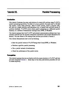
Parallel Processing Techniques for the Processing of Synthetic Aperture Radar Data on GPUs William Chapman, Sanjay Ranka, Sartaj Sahni, Mark Schmalz University of Florida, Department of CISE, Gainesville FL 32611-6120

Abstract - This paper presents a design for parallel processing of synthetic aperture radar (SAR) data using one or more Graphics Processing Units (GPUs). Our design supports realtime reconstruction of a two-dimensional image from a matrix of echo pulses and their corresponding response values. Key to our design is a dual partitioning scheme that divides the output image into tiles and divides the input matrix into sets of pulses. Pairs comprised of an image tile and a pulse set are distributed to thread blocks in a GPU, thus facilitating parallel computation. Memory access latency is masked by the GPU’s low-latency thread scheduling. Our performance analysis quantifies latency as a function of the input and output parameters. Experimental results were generated with an nVidia Tesla C1060 GPU having maximum throughput of 972 Gflop/s. Our design achieves peak throughput of 136 Gflop/s, which scales well for output image sizes from 512 x 512 pixels to 2,048 x 2,048 pixels. Higher throughput can be obtained by distributing the pulse matrix across multiple GPUs and combining the results at a host device.

I. INTRODUCTION The use of electromagnetic waves to produce images that depict detail beyond the response of human vision is of keen research interest for applications such as computed tomography, meteorology and geology (e.g., remote sensing). In particular, radar-based mapping of ground objects can benefit from high performance parallel computing techniques. In practice, radar mapping involves the reconstruction of a two-dimensional image of an object from a collection of radar pulses, together with parameters of the radar sensor. As shown in Figure 1, a device at a known location L emits a pulse at time T0. Reflections (echoes) of this pulse from the target are collected as a function of time over a given interval. Echoes associated with objects further from the emitter will arrive at the sensor later than those closer to the emitter. In Figure 1, the response for P1 will appear at an earlier time than P2, and P2 will appear earlier than P3. The exact time these responses should arrive can be estimated by dividing the distance between L and Px by the speed of light c. Unfortunately, while predicting the arrival time for a given point Pi is relatively simple, the inversion of multiple echoes to determine Pi can be challenging due to ambiguities. For example, as shown in Figure 2, an additional point P4 can have the same distance from L as P1, and can cause an equal response time as P1. Given the response data for a single pulse, one cannot disambiguate the echoes from P1 versus P4, thus confounding reconstruction of P1 versus P4. Instead, one can only approximate the location within the concentric circle centered on L, shown as

Uttam Majumder ARFL/RYAS, Dayton OH 45431

Figure 1: A radar pulse is transmitted, and response intensity is measured as a function of time. Responses from more distant objects traverse a longer path and will return to the sensor at a later time.

Figure 2. Configuration of Figure 1 shown in top view. An object at P4 is the same distance from L as P1, and will have the same response time.

a dotted line in Figure 2. Synthetic aperture radar provides a technique for resolving these spatial ambiguities, based on the exploitation of multiple pulses taken at multiple locations over time, to increase radar sampling density and thus the effective aperture. In the example shown in Figures 1 and 2, the sampling process could be repeated with L in different locations with respect to P1, P2, and P3. Via solution of an inversion equation, the ambiguity between P1 and P4 can be approximately resolved, allowing a more accurate approximation of sensed objects in their reconstructed versus truthed locations. Additionally, the effect of sampling error due to interference and environmental factors is reduced by averaging of multiple replicates. Unfortunately, SAR-based image reconstruction becomes more expensive computationally as the number of pulses and range bins per pulse increases. For example, our experiments showed that a 512x512-pixel image having 42,208 pulses and 4096 range bins per pulse took over four hours to reconstruct on a consumer-grade 2 GHz Centrino processor. Fortunately, the emergence of less expensive parallel architectures offers support for fast but computationally expensive SAR reconstruction, for example, with Graphics Processing Units (GPUs). In addition to efficiency, a GPU’s data partitioning scheme, as well as our optimization strategies for peak throughput, can be generalized to a variety of problems with data access pattern characteristics similar to SAR reconstruction. In particular, our scheme can be effectively applied to generate an effective GPU solution to any problem where spatial locality of output data implies spatial locality of the required input data (for example, in computed tomography). Due to space limitations, we focus the remainder of this paper on SAR reconstruction with one or more GPUs.

II. PRELIMINARIES

Additional detail regarding the backprojection algorithm, and its enhancements, can be found in [3].

1. The Backprojection Algorithm Several algorithms are available for SAR reconstruction from pulse response data, and instances of these algorithms have been optimized to perform well on sequential systems with relatively low throughput. In designing these algorithms, computational performance, rather than quality of the reconstructed image, tended to be the primary evaluation metric. An algorithm that was rated poorly by this metric is the backprojection (BP) algorithm [3]. BP, known for its large computational cost and high output quality, examines the pairing of every received (postprocessed) pulse with every reconstructed pixel to estimate object reflectivity at each point in the spatial representation. The details of this algorithm are beyond the scope of this paper, but the algorithm is summarized as follows. The pulse response data, or pulse response matrix, is partitioned into range bins. Each range bin corresponds to a measured response during a given interval of time after the pulse was emitted. As mentioned in Section 1, responses that arrive later are further from the emitter location, and are thus placed into a higher-numbered range bin. For each pixel in the output image, every pulse, and every range bin in that pulse, is considered separately, with the value in a given range bin being added to the value of the associated pixel of the reconstructed SAR image. Thus, areas of higher reflectivity will be associated with brighter output pixels or regions. More formally, the main computational loop of the backprojection algorithm features the pairing of each pulse in the pulse response matrix with each pixel of the output image. Let P denote the set of pulses, with P[i].bin[j] denoting the jth range bin of pulse i after phase correction, and (P[i].x, P[i].y, P[i].z) denoting the source of pulse i with respect to some fixed reference point. If each pulse has a range of Rstart to Rend, then the intensity of the output image pixel at (x,y) can be written: P

Yx, y =



∑ P[i ].bin 

i=1



(x − P[i ].x )2 + ( y − P[i ]. y )2 + (P[i ].z )2   (Rend − Rstart ) / | P[i].bin | 

(1)



Surprisingly, this model captures the data movement patterns of the backprojection algorithm, although our implementation includes several enhancements to improve output quality. For instance, in Equation (1), it was assumed that pixel (x,y) maps to a range bin indexed by an integer. In practice, pixels often fall between range bins, mapping to bins that have a fractional index. In such cases, an interpolated (smoother) image can be generated by examining range bins adjacent to a fractionally-indexed bin, then computing their weighted average based on their distance from this bin. Such enhancements are not the focus of this paper; we view any implementation of the backprojection algorithm with a data access pattern as shown in Equation 1 as being logically equivalent.

2. Related Work The algorithm and design presented herein are tailored to the fast parallel processing of synthetic aperture radar data,as well as reconstruction of a corresponding two-dimensional SAR output image. However, these techniques could also be applied to any domain where pulse response data is projected back to form an image of a surface, object, or area. One such application is computer aided tomography, or the construction of three-dimensional models from a set of cross-sectional views, for example, for the purpose of obtaining a three dimensional view of tissue in vivo. Here, each atomic volumetric unit or voxel demonstrates the same properties derived from a reconstructed SAR pixel. Namely, for a given cross-sectional view, each voxel will be associated with a response value that is spatially near the response of its neighboring voxel. Similarly, a given volume of output data will require a predictable quantity of response data for each cross section. The preservation of these properties ensures that the proposed partitioning scheme would also provide an efficient data access mechanism for generating tomograms [2,9]. Other potential applications of our algorithm depart entirely from the domain of image sampling. Network tomography, for example, involves the inference of network characteristics from observations taken at a variety of known locations. In this case, each node in the network core is analogous to a pixel in the output image, where each sample location is analogous to a pulse. The latency or reliability of a channel can be inferred from the repeated transfer of packets between locations. The projection of this data back onto the nodes through which packets travelled can produce a visual representation of the network at any point in time, without requiring explicit assistance from core nodes. In this paradigm, spatial locality follows from the route optimization properties of routing protocols [8]. A similar problem involves estimation of ocean temperatures from acoustic wave propagation latencies, because the speed of sound in water is directly related to water temperature. By measuring the propagation time of the wave between a variety of sources and destinations, a set of cross sectional images can be reconstructed that is analogous to the images obtained in computer aided tomography. Small three dimensional units of water, not unlike the voxels of computer aided tomography, become the unit onto which acoustic sensor response data is projected. Spatial locality of input data follows from the output partitioning scheme [10]. 3. Graphics Processing Unit (GPU) A Graphics Processing Unit is a parallel computing device having high throughput and relatively low cost. GPUs can be purchased for less than 100 USD, and are found inside many modern desktop computers. Performance of

GPUs, despite their price, has been measured at over 900 GFLOPs. Comparatively, high end consumer-grade CPUs have not achieved more than 150 GFLOPs per chip [4]. The throughput of GPUs can be attributed to their high degree of parallelism, or more specifically, their ability to operate efficiently as single instruction, multiple data (SIMD) devices. The nVidia Tesla C1060 GPU, which was used in our experiments, has 30 streaming multiprocessors, each consisting of 8 streaming processors or cores, for a total of 240 cores. Generally, GPUs execute threads by arranging them into thread blocks. Each thread block corresponds to the execution of a single piece of code across multiple parallel threads, with each thread acting on a different unit of data. The code running on each thread is referred to as a kernel. During the design phase, a programmer can specify which parts of an application are suited for this type of execution, labeling them as kernels using syntax specified by the GPU language (e.g., CUDA for our nVidia Tesla processor). At runtime, each thread block is capable of accessing a common shared memory device, which allows for a form of inter-thread communication. A much slower device, global memory, is accessible from all thread blocks, and is used to transfer data to and from the host [4]. As in other hierarchically-configured memory systems, high performance implies concentration on local (on-chip) memory operations, with minimal transfer to and from slower storage devices. The GPU is intended to operate efficiently with thousands of threads running simultaneously, since thread scheduling is implemented directly in GPU hardware and has negligible overhead compared to program execution time. In GPUs, the support for numerous threads allows memory access latencies to be masked, since other threads may operate while paused threads wait for IO operations to complete. With respect to SAR, the backprojection algorithm described in the preceding section is an ideal candidate for GPU implementation, since (a) each output pixel can be viewed as the sum of the contribution of each input pulse, and (b) the set of operations used to calculate this contribution is not dependent on the value of the input. III. DATA MOVEMENT ISSUES IN SAR The backprojection algorithm described in Equation 1 requires the computational pairing of each pixel in the output image with each pulse in the pulse response matrix. This requires that each pixel and its corresponding range bin from each pulse must be available on-chip at the same time. Since both the output image and pulse response matrix can be quite large in size, it is often impossible to fit the entirety of either structure in shared memory, constant memory or register memory. Fortunately, the data access pattern of the backprojection algorithm ensures two properties that are helpful in reducing the global memory access. We will appeal to these properties in Section 4.4 when we examine a

Figure 3. The minimum number of range bins needed corresponds to a look angle that is parallel to any side of the square region (L1). The maximum number of range bins occurs at an angle whose incident line forms a 45O angle with each side of the square region (L2). partitioning scheme that attains data access locality in backprojection. Let the function N(P, S) be the number of range bins for a given pulse required to completely generate a square subregion S of the output image. For any square subregion S and pair of pulses (P1 , P2), we have Property 1: Lemma 1: N (P1 , S ) ≤ 2 N (P2, S ) This property can be explained by recalling that the range bin needed for a given pixel is linearly related to its distance from the pulse location. For any two points, the factor relating the difference in their physical locations to the difference D in their corresponding range bins is constant. In particular, D equals the total distance sampled divided by the number of range bins. Observe that the least number of range bins will be required when the look angle is either parallel or perpendicular to the base of the square subregion. Likewise, the maximum number of range bins is required when the look angle equals 45O, such that (2) Bins = B * D where B denotes the length of the square base. For the 45O case, (3) Bins = B * DiagonalLength = B 2 D The final step is proven using the Pythagorean Theorem. A related property involves the relationship between the number of bins needed by two square subregions. Consider two such regions S1 and S2 with base lengths of b1 and b2. Letting P be a pulse in the pulse response matrix, we obtain the following lemma that states Property 2: Lemma 2: N (P, S 2 )b1 ≤ N (P, S1 ) ≤ 2 N (P, S 2 )b1 b2 2b2 Observe that the distance between any two points on opposite boundaries of S1 is less than or equal to B1 2 . This follows directly from the Pythagorean Theorem. The upper bound on the number of range bins required to render this image is then proportional to B1 2 , with a proportionality constant (C, as distinct from the speed of light c) determined by the sampling resolution:

(5) N (P, S1 ) ≤ CB1 2 Likewise, observe that the distance between any two points on opposite boundaries of S2 is greater than or equal to B2. The number of range bins required is then proportional to B2. Since the input pulse data P remains constant, so does the sampling resolution and the (constant) factor C. As a result, we have (6) N (P, S 2 ) ≥ CB2 Observing that B2 is a positive number, N (P, S 2 ) (7) C≤ B2 and the upper bound of Property 2 follows from substitution of C. The lower bound of Property 2 follows directly from the upper bound. By swapping the roles of S1 and S2, and noting that b1 and b2 are positive, we have 2 N (P, S1 )b2 (8) N (P, S 2 ) ≤ b1 and the result follows. IV. APPROACHES FOR DESIGNING A PARALLEL IMPLEMENTATION The Backprojection Algorithm can be implemented on a GPU by defining the kernel as the pairing of one pixel with one pulse. The steps involved in performing this operation are the same for all pixel/pulse pairs, so it is inherently SIMD in nature. However, challenges arise in the mapping of pair/pulse combinations to thread groups. 1. A Naive Approach First, let us consider the simplest approach, where kernels are grouped arbitrarily. (See Figure 4.) Using this scheme, each pulse/pair combination is assigned to a thread in an unspecified sequence. This will produce a correct result, because the backprojection algorithm does not specify an order in which contributions must be summed. It is also relatively easy to implement, as the programmer does not have to concern himself with the details of grouping kernels efficiently. This approach is also practical if the size of the pulse response matrix is small enough to be copied to each shared memory, where each thread has rapid access to the entire pulse response matrix, so it can perform the necessary computations without incurring data movement penalties. When the pulse response matrix is large, it cannot be copied to each shared memory; however, it may still be possible to store the pulse response matrix in global memory. If shared memory is used as a local cache, and the pulse response matrix memory is divided into pages equal to the cache size, a cache hit will occur with an average frequency equal to the size of shared memory divided by the pulse response matrix size. Our analysis shows that this results in only a few cache sits in several thousand projections, even when the image

memory accesses are not considered. Noting that the time required to access a cache page is larger than the time required to read a single byte from global memory, it is preferable to access global memory directly. Global memory access latencies are roughly two orders of magnitude slower than shared memory, so this is not a feasible approach for the implementation of a backprojection algorithm. While this approach achieves the minimum computational requirements of backprojection, it does not take advantage of the GPU memory hierarchy. The cost of moving data from global memory to the GPU multiprocessor is then one pixel load, one range bin load, and one pixel write-back per pixel/pulse combination. Assuming an image size of N x N pixels, rendered using P pulses, this process requires 3PN2 global memory operations. We have found that the only remaining solution is to achieve access locality by partitioning the data and corresponding pixel/pulse combinations, ensuring that only a small subset of the data needs to be copied to shared memory at any one time. For each of the following proposed partitioning schemes, we shall present a global memory access cost in terms of N and P as defined above. Omitting the bookkeeping calculations needed to implement partitioning, all schemes are computationally equivalent. 2. Pulse Response Matrix Partitioning In contrast, if the pulse response matrix is partitioned into blocks row- and column-wise, as shown in Figure 5, then each block and the output pixels associated with this block can be copied to the shared memory, processed, then written back to global memory. This approach initially appears promising, as it results in minimal transfer of the pulse response matrix data: range bins are loaded from memory, projected onto the image, and then discarded as they are not needed in shared memory again. The challenges of this approach are best characterized by considering the requirements of partitioning in each dimension: the range bin dimension and the pulse dimension. Of these, the former is notably more troublesome. The key problem with dividing a pulse's range bins across multiple blocks is the output image data access pattern. In order to fully process the pulse, all pixels to which the elements of this pulse contribute must be stored in memory and updated. Since a single range bin contributes to all pixels at a certain distance from the pulse source, a relatively small number of range bins may correspond to a large number of pixels, as shown in Figure 5. In addition, images are represented in memory as a two-dimensional array of pixels, where the upper left pixel is defined as the starting point, and subsequent pixels are stored in row-major order. Using this scheme, the pixels accessed by each partition of the pulse response matrix rarely occupy adjacent locations in memory. Since the GPU is optimized to load data from memory in vector form, the fact that these pixels are not adjacent and thus cannot be efficiently grouped into

vectors results in high access latencies. For these reasons, it is preferable not to partition along this dimension. Pulse response matrix partitioning should only be considered as a technique that divides the data structure into groups of pulses. If pulses are blocked in this manner, access locality on the pulse response matrix is achieved within each block. However, each pulse contributes to every pixel in the reconstructed image. There is no access locality on the output image. It follows that the global memory access cost of this scheme is a single transfer of the pulse response matrix followed by one pixel load and one pixel store for each pixel/pulse combination. Referring back to our definitions of N and P, and defining R to be the number of range bins per pulse, this cost is PR + 2PN2. Fortunately, it is possible to reduce the burden of the pixel load and writeback steps if enough space is available to locally store an independent copy of the output image for each pulse block. After completing the block, the output can be summed with the image already residing in global memory in a single pair of load and write-back memory transactions. This final step represents a reduction operation that produces a single output image from the output of each pulse block. The global memory access cost of this improved scheme, where S is the number of pulse blocks, is PR + 2SN2. Although this technique is helpful in reducing the I/O cost of backprojection, it imposes global memory access requirements and on-chip memory requirements that are sensitive to the size of the output image. Additional partitioning is necessary to achieve reasonable performance when the size of the output image is large.

Figure 4. Data access pattern when each thread block is assigned an arbitrary collection of pixels. There are is no locality of access to be exploited on either the pulse response matrix or the output image, so each thread must have random access to the entirety of both data structures.

Figure 5. Partitioning the pulse response matrix data is an effective technique that permits pulse data to be loaded into shared memory, used, and then discarded. However, the required image pixels are within a specfic distance interval of a given pulse. These pixels do not occupy adjacent memory locations, and demonstrate poor access locality.

3. Output Image Partitioning Rather than perform a block partition on the pulse response matrix, another approach involves partitioning the output image, as shown notionally in Figure 6. Using this approach, the output image is divided into tiles, and each tile is rendered by a single processing element. In [5], we have shown this is an efficient means of implementing the Proximality means that, for a pair of nearby pixels X and Y, the range bins needed to compute X are proximal (near) in the pulse response matrix to those range bins required to compute Y. This permits FPGA implementations to route data through a spatially-mapped algorithm in nearly systolic fashion, facilitating high throughput with relatively low hardware costs. It also encourages the selection of a tile size that is relatively small with respect to the size of the output image. This advantage occurs because the underlying data structure benefited from the property of proximality, and performed more effectively when all pixels in the tile were reasonably close together. This property is not helpful in a GPU due to its shared memory architecture, and due to the fact that a small tile size results in pulse data being loaded from memory more frequently. In contrast, GPU implementation tends to favor large tile sizes, which reduce the amount of unnecessary

Figure 6. Partitioning the output image into small tiles supports locality of access for input and output data. Each small subimage corresponds to a vertical strip of the pulse response matrix. pulse data movement. The global memory access cost of this scheme is the cost of transferring a subset of the range bins from each pulse to the processing element rendering each tile, followed by a write-back of the tile to global memory after generation is complete. There is no reduction step because each tile represents the contribution of all pulses in the pulse response matrix, rather than a subset of pulses. As shown above, each tile requires a number of bins that is proportional to K/N, so the global memory access cost scales with PRN/K + N2. A factor of 2 does not precede the N2 term because the writeback operation does not require a load step, as no reduction

operation is occurring. This equation shows that larger tile sizes inherently incur lower global memory access costs. A range bin is copied from global memory each time it is needed by a tile. As the set of pixels contributed to by a range bin increases, the number of times that bin must be copied from global memory also increases. 4. Output Image and Pulse Response Matrix Partitioning While large tile sizes help reduce I/O cost, they also reduce algorithmic parallelism. When the image size is small relative to the tile size, there are fewer partitions to be distributed across the available processing cores. An inefficient partitioning scheme results. Memory access delays that would be masked by a larger number of partitions instead adversely impact device throughput. This challenge can be overcome by splitting the pulses into pulse sets, then distributing the computation of a single image tile across several cores. Using output partitioning only, each thread handles the computation of a set of pixels across all pulses. Thus, a thread now computes a set of pixels across 1/S pulses, where S is the number of pulse sets. Figures 9 and 10 illustrate this approach notionally, comparing it with a pure output partitioning scheme. Thus, the previous approach is simply a specialization of this approach with S=1. Because this approach partitions the pulse response matrix, each tile of the output image is further distributed across processing devices. This requires a load and write-back reduction step as described in Section 4.2, increasing the global memory access cost to PRN/K + 2SN2. In this equation, the value of P, R and N are input parameters to backprojection, while the values of K and S are variable and can be configured to maximize throughput. An ideal tile size (K) balances unnecessary global memory access (incurred by small tile sizes) against decreased parallelism (observed for large tile sizes). Unnecessary global memory access occurs when the same range bin from a given pulse is transferred from global memory to shared memory more than once, as occurs when a range bin is used for multiple pixels in different tiles (as shown in Figure 9). Here, two pixels equidistant from the emitter are assigned to the same range bin. In general, if there are R range bins, and NxN output pixels, then a range bin is accessed, on average, by N 2 / R pixels. In a simple worst case analysis, the tile size K = 1 is equivalent to rendering each pixel independently, thereby accessing global memory each time a range bin is accessed, which results in each bin being loaded N 2 / R times. Considering an image size of 512 x 512 pixels, and our sample data set having 4096 range bins per pulse after oversampling, this results in the pulse response matrix being loaded from memory 64 times. In contrast, a simple bestcase analysis uses K = N, where the entire pulse matrix is loaded from global memory once, used for every pixel of the output image, then permanently discarded, such that the

Figure 7. The output image, represented by the cube face, is partitioned into K x K tiles for distribution across multiple processing units. Each processing unit renders a single tile for each pulse sequentially.

Figure 8. A generalization of the approach described in Figure 7. The pulse set is divided into three groups. Each thread group renders a K x K tile of the output image with respect to 1/3 of the pulses. pulse response matrix is loaded only once. An intermediate case employs Lemma 2, and redefines R as the number of bins needed to render the NxN–pixel image for an arbitrarily chose pulse. In practice, this new value of R may be less than the total number of range bins in that pulse. Without loss of generality, since unused range bins are not transferred to shared memory, they can be ignored when optimizing implementation parameters. If an NxN image is partitioned into KxK tiles, then loading each tile from global memory accesses a predictable number of bins. In particular, consider the case of an image whose x or y axis is incident to the look angle. Here, the number of bins accessed is RK / N . Lemma 2 claims that for any other image tile, the number of range bins required to render this pulse is less than 2 RK / N . Observe that Lemma 2 does not require that the subregions on which it operates (S1 and S2) be contained within the NxN image, nor does it require that they have the same orientation. As a result, for every pulse, there exists a region S1 whose x- or y-axis is incident to the look angle. Therefore we have an upper bound on the number of bins required to render any tile using any pulse. Applying this concept to the processing of every tile in an

NxN image results in a total transfer of bins that is contained within the following interval:  RN 2 RN  , (9)    K , K    as shown in Figure 9 using 4096 range bins and 512 x 512 output pixels. From the previous relationship, it would appear that an optimal tile size is K = N, subject to memory constraints. However, we have already shown this is not the case. Large values of K, even in environments where memory is not limited, reduce the inherent parallelism of the tiled approach. On a GPU, where many processing cores are available for parallel operation, this situation is inefficient. In particular, since only one thread block is being rendered at a time, the reconstruction operation is restricted to a single multiprocessor, and the GPU is forced to pause computation during the operations that read and write from global memory. If a larger number of thread blocks were available, then the GPU could interleave computation and memory access, significantly masking these latencies. Thus, a second partitioning scheme was introduced on the pulse dimension of the pulse response matrix. The characteristics of this partitioning scheme can be observed graphically. Figure 10 describes the observed latency when tile size is selected to be the size of the output image. This results in minimal parallelism, since only one block is being rendered by a single multiprocessor. It also results in minimal pulse response matrix data transfer, as described in the preceding analysis. The shape of this graph indicates that increasing the number of pulse partitions initially has the effect of decreasing latency. Beyond some optimal point, latency begins to increase at a rate that is linear with respect to the number of pulse sets. In order to maximize throughput, we analyze in greater depth the shape of Figure 10. Firstly, we consider the downward slope of the graph caused by increased parallelism from larger numbers of threads. As shown in Figure 11, this graph can be divided into three distinct regions. In Region 1, the GPU is underutilized, as there are not enough thread blocks to distribute to the multiprocessors. Increasing the number of blocks results in a linear decrease in the latency. In Region 2, there are enough thread blocks to distribute to every multiprocessor. However, some multiprocessors have only a small number of blocks assigned to them. When the threads in these blocks block to wait for global memory access, the multiprocessor has no other work to do and must wait until memory access is complete. During this time, the multiprocessor is idle, yielding suboptimal latencies. In Region 3, ample work is distributed among the device, so multiprocessors rarely go idle. The upward-sloping element of the graph results from the reduction operation at the completion of each image block. When the pulse response matrix is distributed to several blocks, the images

Figure 9. The pulse response matrix data transfer bounds (Equation 9) are modeled as a function of tile size K. The required number of range bins is 4096, and the output image is 512x512 pixels. Larger tile sizes result in less movement of pulse response matrix data.

Figure 10. Latency response for reconstructing an N x N image, where K = N, and the number of pulse sets is varied from 1 to the logical maximum of 1 pulse per pulse set. Latency decreases sharply as parallelism improves, then increases as the latency to reduce output images overtakes improvements from increased parallelism. generated by each block must be combined to form a final output image, using the transfer medium of global memory. This global memory access cost increases with the number of output images, which results in a linear increase in latency as the number of pulse sets is increased, per Figure 12. 4.5 - The Effect of Input and Output Size From the preceding analysis, when image sizes are large with respect to the pulse response matrix, it is desirable to use a smaller tile size and recycle the pulse response matrix through global memory. When image sizes are small with respect to the pulse response matrix, large tile sizes are preferred, and pulse partitioning is the preferred means of

achieving parallelism. This follows from the notion that small tile sizes result in more unnecessary global memory access on the pulse response matrix, per Figure 9, and large tile sizes dictate the need for pulse partitioning and image reduction, per Figures 13 and 15. Modern GPU devices contain a relatively small block of low latency memory. This provides an upper bound on the tile size that does not limit computation parallelism on the smallest image size of 512 x 512. As a result, pulse partitioning is not used to obtain our experimental results. However, we anticipate this optimization will be of increased importance in future devices. V. EXPERIMENTAL GPU IMPLEMENTATION GPUs are convenient architectures for implementing tilebased partitioning, since most GPUs provide native support for two-dimensional block partitioning by allowing thread groups to be indexed on a two dimensional grid. This supports logical correspondence between the thread partitioning and image partitioning schemes. Also, each thread group evaluates one tile of the output image, as shown in Figure 6. A GPU can also permit thread indexing within each thread group. This provides an equally simple approach for assigning pixels to threads. In particular, the index of each thread is equal to the index of each image pixel, when pixels are traversed in normal scanning order (left to right, top to bottom). Unfortunately, the GPU employed in our experiments supports a maximum of only 512 threads per block. If one thread evaluates each pixel, then this limits the size of the tile to K = 5121/2 = 22, which yields high I/O latency for typical output size, since pulse data is recycled from global memory several times. A better approach assigns each thread multiple pixels to be evaluated sequentially, as summarized in Figure 14. Distribution of the pulse data is facilitated by the fact that the reconstruction of a given output pixel with respect to each pulse is an independent event. As a result, no benefit is gained from loading multiple pulses into shared memory at a single time. Except in the rare instance that there are not enough pixels to occupy the group threads, there is no possibility of rendering two pulses in parallel within a single thread group. Even in such an instance, there is no performance benefit to be seen from loading multiple pulses, since greater efficiency could be achieved by increasing the tile size or reducing the number of threads in the group. As a result, a more effective technique allows each thread to render each set of pixels with respect to every pulse. When the computation of each pixel-pulse pair is treated as a tuple in three dimensional space, this technique can be depicted as shown in Figure 8. The approach benefits from its simplicity: each pixel can be stored either in a register or in shared memory, so at the completion of the thread, there is no additional work to be done. A completed pixel value is

Figure 11. The latency of increasing the number of pulse sets being computed in parallel, excluding the reduction operation used to generate a final result. Regions 1-3 are illustrated notionally.

Figure 12. Reduction latency increases as the number of pulse sets computed in parallel is increased. The slope of the increase is the size of the image divided by the bandwidth of global memory.

Figure 14. Output image decomposed into two-dimensional KxK-pixel tiles, where each tile is evaluated by one thread block. To accommodate tile sizes larger than K = 5121/2, each thread can process a set of pixels sequentially. available for immediate copying back to global memory. In order to achieve maximal throughput, other factors affecting GPU performance were considered. In particular, performance is maximized when global memory accesses occur in a pattern that facilitates memory coalescing. Coalescing describes the ability of the GPU to group multiple memory requests into a single memory transaction when certain criteria are satisfied. GPU devices of compute capability 1.2 or higher, which include the device on which our experiments were performed, are capable of coalescing 16 transactions of transfer from global memory when all threads in a half warp access 4 byte or 8 byte words and all words are located in the same memory segment. To satisfy this requirement, the contribution of each pulse to a tile is split into three parts. Each thread in a block performs the following steps: for each pulse { // compute the minimum and maximum // range bin needed by the pulse // copy the range bins from global // memory to shared memory // compute the contribution of the // pulse to the pixels handled by // this thread }

The second step is ensures that the requirements for coalescing are met. Each thread accesses the bin equal to the minimum range bin summed with its thread id. If the number of bins needed exceeds the number of threads in the block, a pointer is moved to the last bin read and the process is repeated. This approach is effective in ensuring that pulse data is coalesced. However, it does not achieve coalescing for pulse meta-data. This includes the pulse location, frequency, and range. The pulse location consists of an x, y, and z coordinate, each represented by a single float. Likewise, the frequently and range also occupy a single float. Each of these five data items are stored in separate arrays. This excludes the possibility of coalescing unless the meta-data for multiple pulses are loaded in a single transaction. For that reason, the loop in the code segment above is split into two loops as follows: for each set of 64 pulses { //load x position for all pulses in set //load y position for all pulses in set //load z position for all pulses in set //load frequency for all pulses in set //load range for all pulses in set for each pulse in set { // compute the minimum and maximum // range bin needed by the pulse // copy the range bins from global // memory to shared memory // compute the contribution of the // pulse to the pixels handled by // this thread } }

In modern GPU devices, the performance of coalescing can be improved by increasing the word size of the data being coalesced. In particular, by packaging pulse data and pulse meta data into the GPU's float4 data type, we were able to obtain noticeably higher global memory bandwidth. A global memory access that does not implement this optimization is coded as follows: shared[threadIdx.x] = global[threadIdx.x + offset];

The same memory access, rewritten to implement 16 bit word coalescing, would be modified to the following. The global array in this code has been cast to an array of type float4, which is reflected in the use of the identifier global4 in place of global.

The increase in the size of each element in the global memory array has the effect of multiplying the index accessed by four. To preserve correctness, corresponding adjustments must be made to the offset value and shared memory index. The GPU has also been shown to perform more efficiently when multiple blocks are active on each multiprocessor. This permits global memory access latency to be masked by overlapping execution with reads. A block can be marked as active on a multiprocessor if there are enough shared memory resources and registers available to service the block. The GPU used for our experiments contained 16 KB of shared memory and 16384 registers per multiprocessor. It was necessary, therefore, to ensure that each block used less than half those resources. The allocation of shared memory to meet these requirements was not difficult. Using the analysis described in Section 3, our experimental data, and a tile size of 32 x 32, we determined that the maximum number of range bins that could be needed to render a pulse. This data fit easily within 4 KB, leaving an additional 4 KB shared memory per block available for caching pulse meta data. The process of register allocation, however, proved more challenging. Due to the fact that the scope of a register variable is limited to only one thread, a block consisting of 512 threads is limited to only 16 registers per thread if it is intended to share a multiprocessor with another block. This value is prohibitively low, and several optimization techniques were used to reduce register utilization. The first approach was to unroll loops when the number of iterations the loop will execute is known at the time the application is compiled. This has the effect of freeing up the register that would otherwise be used to maintain the loop index. For example, a simple piece of code which computes the sum of the first 3 elements in an array could be implemented as: x = arr[0] for(i=1; i < 3; i++) x += arr[i];

The code segment above requires a register to maintain the value of the index variable i throughout the duration of loop. An alternative implementation, which does not require an index variable, is: x = arr[0]; x += arr[1]; x += arr[2];

float4 temp; temp = global4[threadIdx.x + offset/4]; shared[threadIdx.x*4] = temp.x; shared[threadIdx.x*4+1] = temp.y; shared[threadIdx.x*4+2] = temp.z; shared[threadIdx.x*4+3] = temp.w;

In our experimental implementation, this technique was used to facilitate the sequential computation of several pixels by a single thread without the use of an index register to track which pixel was currently being computed. When parameters to execution are not known at the time of compilation, it is natural to compute them dynamically

and store the results in a variable for later reuse. We have found, however, that this practice can adversely affect the behavior of the register allocator. In many instances, the temporal cost of recomputing a value each time it is needed is outweighed by the spatial cost of allocating a register to hold it. For example, the contribution of a pulse to a pixel is computed as the weighted mean of the range bin immediately preceding the pixel and the bin immediately following it. This contribution is computed twice, once for the real component of the pulse data, and once for the imaginary component. A natural implementation is to determine constants, w1 and w2, whose values range between 0 and 1 depending on where the pixel is located relative to the starting point of the two bins: bin1, the range bin whose boundary immediately precedes the pixel location; w1, ranges between 0.0f and 1.0f, where 1.0f corresponds to pixel that falls exactly on the boundary of bin1. w2 = bin2 real imag

1.0 - w1; = bin1 + 1; = w1 * real[bin1] + w2 * real[bin2]; = w1 * imag[bin1] + w2 * imag[bin2];

The implementation above requires registers to store w2 and bin2. Recomputing these variables reduces register utilization at the expense of increased latency. Consider the following alternative implementation: real = w1 * real[bin1] + (1.0 - w1) * real[bin1 + 1]; imag = w1 * imag[bin1] + (1.0 - w1) * imag[bin1 + 1];

The revised code above frees two registers and requires 2 extra operations. In this instance, the disincentive for implementing this optimization is relatively low, as 2 operation delays is not likely to produce a noticeable effect on performance. In the general case, however, the penalty for recomputing known values may be more severe, and careful analysis is needed to determine if the benefit is worth the cost. A register utilization reduction can also be achieved by reducing the number of threads in a block and increasing the number of pixels rendered by each thread. This follows from the fact that not all registers used by a thread store information about a specific pixel. Many store information about the state of the thread. Therefore, increasing the number of pixels the thread is responsible for does not increase the demand for these registers. One such register corresponds to the variable holding the index of the pulse that is currently being rendered. This register contains information about the state of the thread, not the pixel. Consequently, reducing the number of threads results in a linear decrease in the number of these registers being used. This dramatically reduces thread utilization, at the expense

of thread count. In practice, we determined that the number of threads could be reduced from 512 to 128 without adversely effecting performance. In this environment, each thread handled 8 pixels. A final consideration in obtaining optimal performance is the implementation of transcendental functions. The backprojection algorithm includes one tangent operation per pulse-pixel pair. Evaluating this operation in single precision is costly on a GPU because the approximation algorithm is not well suited for SIMD parallel execution. Fortunately, the GPU includes a much faster implementation of the tangent function, __tanf(). This function evaluates with less precision than the single precision alternative, tanf(). However, despite its higher performance, the substitution of __tanf() in place of tanf() does not adversely affect the output image. The subtraction of an image generated using the faster implementation from an image generated using the single precision implementation resulted in a difference of less than 1 x 10-7 %. For the purpose of comparison, we also implement tangent using a lookup table with 1024 entries. This yielded higher latency than the __tanf() function and produced an output image that differed from the single precision image by 0.02%. VI. EXPERIMENTAL RESULTS The algorithm described above was implemented and tested on an nVidia Tesla C1060 GPU, using publiclyavailable data [12] having 42,208 pulses with 4096 range bins per pulse. Experimental results are shown in Table 1. The low latencies produced by our algorithm, and the analysis provided in the preceding section, support the reconstruction of images in real time using multiple parallel GPU devices as pulse data is collected. For a 512 x 512 pixel output image, reconstruction times of less than one second can be obtained using only four GPUs. For larger tile sizes, the number of GPUs required to obtain such latencies is higher, because the reduction step (discussed previously) takes longer to compute. This can be attributed to the increased number of partial output images to be summed, and the increased size of each image. Table 1 does not include the time required to transfer input pulse data from the host to the GPU and transmit image data back to the host. These times are included in Table 2, and are a function of the bandwidth of the host-GPU connection. In certain environments, however, these times can be masked using the Tesla GPU’s asynchronous invocation capabilities. In particular, since GPU kernel calls and data transfers can be flagged to return prior to completion, it is possible to overlap these instructions. In the case where the entire input pulse response matrix resides in host memory prior to execution, it is possible to load only a small number of pulses, launch a kernel using only those pulses which have been loaded, then continue loading the remainder of the pulses. In this way, the computation process can be overlapped with the startup transfer time. This is a

particularly natural approach for invoking the kernel when pulse data is being read directly from an incoming data stream and reconstruction occurs in real time. In that case, a portion of the pulse data is transferred to the GPU (or one of several GPUs operating in parallel as described in the previous section), the kernel is invoked on those pulses, and computation begins as the next block of pulse data is streamed into global memory for the next computation. This technique was implemented in our test environment, with results shown in Table 2. The latency required to transfer the input data from host memory to GPU global memory was measured to be 1.8 sec. The size of the input data was 1.32 GB, which yielded a host-GPU bandwidth estimate of 732 MB/sec. In addition, due to the fact that all output image sizes must be rendered using the entire pulse response matrix, the host-GPU transfer latency represents a fundamental limit on output latency that is independent of image size. Asynchronous I/O allows most of the transfer latency to be overlapped with computation, but total latencies lower than the transfer latency cannot be obtained. A similar technique can be used to mask the transfer of the output image back from GPU memory. However, this is not particularly useful, as the time required to transfer an image back to the host is usually negligible compared to the other latencies involved in reconstructing the image. For example, a 2048px x 2048px image was reconstructed in 48.1 sec, but required less than 0.1 sec to transfer back to the host device. 1. GPU Implementation Observations Based on our experimental results, a GPU is an ideal architecture for reconstructing SAR images via backprojection. This is primarily due to two key benefits of the GPU architecture: (1) the ability to mask memory access latency through overlapping I/O and computation, and (2) parallelism obtained from 240 cores operating simultaneously. When compared to a consumer grade CPU, the performance difference is dramatic. Tables 3 and 4 depict the Image Size (px)

Tile Size (px)

Lat. (sec)

Throughput (Gflop/s)

512 x 512

32

3.44

119

1024 x 1024

32

12.6

130

2048 x 2048

32

48.1

136

Table 1. Minimum measured reconstruction latencies for three representative output image sizes, in addition to the optimal tile size and number of pulses assigned to each thread block. This table omits the latency required to transfer pulses from the host to the nVidia Tesla C1060 GPU, which is shown in Table 2. Equivalent throughput in Gflop/s is given for each tile.

Without Asynchronous I/O

With Asynchronous I/O

Image Size (px)

Lat. (sec)

Throughput Lat. Throughput (Gflop/s) (sec) (Gflop/s)

512 x 512

5.24

78.3

3.84

107 Gflop/s

1024 x 1024

14.4

113

13.0

126 Gflop/s

2048 x 2048

49.9

131

48.5

135 Gflop/s

Table 2. Minimum measured reconstruction latencies for three image sizes shown in Table 1, including external I/O latency (data transfer between the host and GPU). Based on these observations, bandwidth between the host and GPU in our environment is 732 MB/sec. No Tile Partitioning Image Size (px)

Tile Size 40px x 40px

Lat. Throughput (sec) (Gflop/s)

Lat. (sec)

Throughput (Gflop/s)

3170

0.129

3100

0.132

1024 x 1024 11736

0.140

11485

0.143

512 x 512

Table 3. Minimum measured latencies when images were reconstructed on desktop PC containing an AMD Athlon 64 Dual Core 2.8 GHz Processor, and 2942 MB RAM, utilizing only one computation thread. The L1 cache size per core was 128 KB and the L2 cache size was 1024 KB. The marginal benefit of partitioning when using this architecture is depicted by comparing the latencies observed when the algorithm is run using a tile size of 40 x 40 to the latencies observed when partitioning is not used. No Tile Partitioning Image Size (px)

Tile Size 40px x 40px

Lat. Throughput (sec) (Gflop/s)

Lat. (sec)

Throughput (Gflop/s)

1550

0.265

1510

0.272 Gflop/s

1024 x 1024 5740

0.286

5490

0.299 Gflop/s

512 x 512

Table 4. Minimum measured reconstruction latencies for two cases in Table 3, but with four threads.

throughput when images were rendered on a Windows Vista PC containing an AMD Athlon 64 Dual Core Processor 2.8 GHz, with 2942 MB RAM, 128 KB L1 cache, and 1024MB L2 cache. When images were rendered in a single execution thread, a maximum throughput of 0.132 Gflop/s was obtained. Increasing the number of threads to four and introducing a tiled partitioning scheme increased throughput to 0.299 Gflop/s. Utilizing a larger number of threads was ineffective, as thread scheduling on a CPU is much slower than on a GPU, and the increased latency due to thread scheduling negatively impacts throughput. The impact of tile-based partitioning on throughput is less clear in the CPU than in the GPU. This can be attributed to the large L1 cache size available to the CPU. An entire row of the pulse response matrix from our data set had a size of 32 KB. This fit easily into the L1 cache of the CPU, meaning that pulse response matrix cache misses were rare, even when tile partitioning was not used. The benefit of tile-based partitioning is more pronounced when execution times are measured on a GPU that is not implementing this scheme. An alternative scheme was implemented where each GPU thread operated on a single pixel. This scheme did not partition the output image deliberately, but simply assigned pixels to threads sequentially in a row-major order. This is a variation of the approach described in Section 4.1, except that sequential thread assignment replaces random assignment. For the 512 x 512 pixel output image, a minimum latency of 20.5 sec was obtained, which corresponds to an estimated throughput of 20.0 GFLOPs, well below the measured throughput of 119 GFLOPs obtained using tile based partitioning. The GPU implementation of the tile based partitioning scheme is the superior approach for reconstructing SAR images. Compared to the CPU implementation, the speedup observed from this approach was 438. In contrast, when compared to the inferior GPU partitioning scheme, the speedup was 5.8. VII. CONCLUSIONS AND FUTURE WORK We have presented a design for an efficient mechanism for reconstructing images given synthetic aperture radar data using the Graphics Processing Unit (GPU). Our design, which is optimized for use on the nVidia Tesla C1060 GPU, partitions the output image into tiles. In particular, our approach relies on the fact that the amount of response data required for processing each tile is predictable and proportional to the size of the tile divided by the size of the image. Each thread block in the GPU operates on one tile for a given set of pulses from the pulse response matrix. The optimal tile size is the largest tile such that a single pulse can be contained in GPU shared memory, while still producing enough threads to permit the GPU to effectively make use of its 240 cores. Throughput is limited by the relatively high latency of accessing global memory on the GPU, particularly for

reading the large pulse response matrix into shared memory. Nonetheless, performance for large output images (2048 x 2048 pixels) was measured at up to 136 GFLOPs, which is more than ten percent of the C1060's peak performance measurement of 936 Gflop/s. Lower resolution images (e.g., 512 x 512 pixels), which require a smaller number of computations using the same set of input pulse data, performed at 119 Gflop/s. Our continued research will investigate how multiple GPUs can be configured to operate in parallel and obtain additional throughput. In this case, the computational burden could be distributed across devices using the principles established in Sections 4.1 - 4.5. For small images, an efficient partitioning scheme would distribute blocks of pulses to multiple GPUs and combine the results at a single host machine to form a completed image. For large images, is is likely that a tiled partitioning scheme would be used to distribute image tiles, and the corresponding subset of the pulse data, to each device. Experimental results show that real-time data processing is possible for 512 x 512 pixel images using a small number of GPUs. ACKNOWLEDGEMENTS The authors gratefully acknowledge support of this work under Air Force contract #FA8650-09-M-1563 and NSF grant NETS 0963812. REFERENCES [1]

Mita

D. Desai and W. Kenneth Jenkins, "Convolution Backprojection Image Reconstruction for Spotlight Mode Synthetic Aperture Radar" IEEE Transactions on Image Processing, Vol. 1 No. 4, pp. 505-517, 1992. [2] Nicolas Gac and Stephane Mancini and Michel Desvignes and Dominique Houzet, "High Speed 3D Tomography on CPU, GPU and FPGA" [3] Lars M. H. Ulander, Hans Hellsten, Gunnar Stenstrom, "Synthetic-Aperture Radar Processing Using Fast Factorized Back-Projection" IEEE Transactions on Aerospace and Electronic Systems, Vol. 39 No. 3, pp. 760-776, 2003. [4] "NVIDIA Programming Guide - Version 2.2." April 2009. [5] William Chapman, Sanjay Ranka, Sartaj Sahni, Mark Schmalz, "Parallel Processing Techniques for the Processing of Synthetic Aperture Radar Data on FPGAs." October 2009. [6] Shibdas Bandyopadhyay, "SAR implementation on the GPU using CUDA." August 2009. [7] "Introduction to CUDA", NVidia Corp 2008 [8] "Network Tomography: estimating source-destination traffic intensities from link data". J. Am. Statistics Association 91: 365-377. 1996 [9] R.S. Ledley, Introduction to computerized tomography, Comput. Biol. Med. 6 (1976), pp. 239–246. [10] Brekhovskikh, Leonid. Fundamentals of ocean acoustics. 3rd. Springer Verlag, 2003. Print. [11] Alan Dl Cenzo, "A Comparison of Resolution for Spotlight SyntheticAperture Radar and Computer-Aided Tomography" Proceedings of the IEEE, VOL 74, NO. 6, Aug 1966 [12] Curtis H. Casteel, Jr, LeRoy A. Gorham, Michael J. Minardi, Steven M. Scarborough, Kiranmai D. Naidu, Uttam K. Majumder. "A Challenge Problem for 2D/3D Imaging of Targets from a Volumetric Data Set in an Urban Environment." Proc. of SPIE Vol. 6568 65680D-1