238. IEEE TRANSACTIONS ON COMPUTERS, VOL. 38, NO. 2, FEBRUARY
1989. Parallel Sorting in Two-Dimensional VLSI Models of Computation.
238
IEEE TRANSACTIONS ON COMPUTERS, VOL. 38, NO. 2, FEBRUARY 1989
Parallel Sorting in Two-Dimensional VLSI Models of Computation Abstract-Shear-sort opened new avenues in the research of sorting techniques for mesh-connected processor arrays. The algorithm is extremely simple and converges to a snake-like sorted sequence with a time complexity which is suboptimal by a logarithmic factor. The techniques used for analyzing shear-sort have been used to derive more efficient algorithms, which have important ramifications both from practical and theoretical viewpoints. Although the algorithms described apply to any general two-dimensional computational model, the focus of most discussions is on mesh-connected computers which are now commercially available. In spite of a rich history of O ( n ) sorting algorithms on an n x n SIMD mesh, the constants associated with the leading term (i.e., n ) are fairly large. This had led researchers to speculate about the tightness of the lower bound. The work in this paper sheds some more light on this problem as a 4n-step algorithm is shown to exist for a model slightly more powerful than the conventional SIMD model. Moreover, this algorithm has a running time of 3n steps on the more powerful MIMD model, which is “truly” optimal for such a model. Index Terms-Distance bound, lower bound, mesh-connected network, parallel algorithm, sorting, time complexity, upper bound. I. INTRODUCTION
T
WO-DIMENSIONAL sorting is defined as the ordering of a rectangular array of numbers such that every element is routed to a distinct position of the array predetermined by some indexing scheme. Some of the standard indexing schemes are illustrated in Fig. 1. The simplest computational model onto which this problem can be mapped is the meshconnected processor array (mesh for short). The simplicity of the interconnection pattern, and the locality of communication, makes the mesh easy to build and program and was the basis of one of the earliest parallel computers (ILLIAC IV). Since then, there have been more machines built on a much larger scale including the MPP and the DAPP using similar interconnection patterns. This simple architecture further motivates the idea of dealing with a given set of numbers as a rectangular array rather than as a linear sequence. More recently, Scherson [15] and Tseng et al. [22] have independently proposed a network which they call the orthogonal access architecture and the reduced-mesh network, respectively. It consists of p processors which are connected by a shared memory of p - q x p - q locations, where each Manuscript received August 29, 1986; revised February 15, 1988. I. D. Scherson is with the Department of Electrical Engineering, Princeton University, Princeton, NJ 08544. S. Sen is with the Department of Computer Science, Duke University, Durham, NC 27706. IEEE Log Number 8824537.
g 13
(b)
Fig. 1. Some indexing schemes. (a) Row major, @) snake-like row major, (c) shuffled row major.
processor can randomly access a row or a column of size q independently. The sequential complexity of sorting has been studied extensively for well over two decades (for a very interesting account of the history of the development of various sorting methods, see [4]) but only recently has the complexity of parallel sorting received much attention. Although several interesting results have been obtained for various PRAM models (for example, see Reischuk [12], Cole [2]), the existence of a practical O ( n )processor O(1og n ) depth sorting network remains unresolved. The O(1og n ) depth AKS network ([ 11) and the subsequent improvement in processor bound by Leighton [8] are primarily of theoretical importance. A trivial lower bound for sorting on any network is imposed by the diameter of the network which implies an Q ( n ) time complexity for sorting on an n x n mesh The restriction on parallelism imposed by the nearest-neighbor type interconnection results in inferior performance of algorithms on the mesh versus networks like the shuffle-exchange, the hypercube, etc., which have smaller diameters due to more complicated interconnection patterns. This is a price that one pays for simplicity of the network interconnections which may be worthwhile for a large number of applications. In particular, the recent interest in systolic implementations is based on a family of nearest-neighbor type interconnections of which the mesh-connectedprocessors is one of the simplest assemblages. One of earliest results for sorting on rectangular arrays of numbers was published by Thompson and Kung [20]. The
’.
’
In future, all references to “mesh” will imply an n x n array of processors. All logarithms are to the base 2.
OO18-9340/89/0200-0238$01.OO O 1989 IEEE
239
SCHERSON AND SEN: PARALLEL SORTING IN TWO-DIMENSIONAL VLSI MODELS
model of computation chosen was a mesh-connected array of processors without wrap-around connections and operating in a strict SIMD mode. Their efforts were soon followed by Nassimi and Sahni [lo], and Kumar and Hirschberg [5] who presented algorithms with improved constant factors. More recently, Lang et al. [7], and Schnorr and Shamir [18] published e(n) algorithms for a stronger model. Table I shows the results of these papers in terms of the time complexity, computational model, and the indexing scheme of the sorted sequence. Note: For most parts in this paper, the expressions for time complexities will only contain the asymptotically dominating term. In other words, time complexity of the form kn, where k is a constant will be used to imply kn + o(n). While comparing the relative merits of these algorithms, one has to be extremely careful about the precise model of the mesh. The two most commonly used models are the SIMD (proposed by Thompson and Kung [20]) and the MIMD (initially used by Lang et al. [7] and later characterized more formally by Schnorr and Shamir [ 181). The MIMD model is considerably more powerful that the SIMD model since it allows a conditional exchange between nearest neighbors in one step and does not distinguish between a comparison and a routing step. This is somewhat unrealistic since the time for comparing two “b” bit words is a function of b, whereas routing between nearest neighbors can be done in constant time using bit-parallel communication. Thus, strictly speaking, any algorithm that uses O(n)comparison steps cannot be considered optimal in an SIMD model because the lower bound is 4(n - 1) unit routing steps. Table 111, in Section IV-B, compares the time complexities of some algorithms of Table I when mapped into different models of computation. The plethora of results for “optimal” algorithms on the mesh reflects widespread suspicion that there is scope for improvement, especially in the constant factor of the leading term. The problem for the MIMD model was settled to some extent by the recent results of Kunde [6], and Schnorr and Shamir [ 181, who (independently) proved a lower bound of 3n steps for row-major indexing and also presented algorithms matching this bound. (Kunde [6] actually showed that the s2merge algorithm of Thompson and Kung [20] is optimal in the MIMD model.) The problem of proving a tight lower bound in the SIMD model appears to be more formidable. The trivial distance bound of 4n steps (needed to interchange two elements from the opposite corners) has not been matched by any algorithm so far. The best known running time for the SIMD model is 7n routing steps which is achieved by one of the algorithms presented in this paper (and also by a modification of Thompson and Kung’s algorithm). A more in-depth study of the past algorithms shows that they can be broadly classified into two approaches. The earlier efforts were adaptations of inherently parallel algorithms like odd-even merge and bitonic sort to the mesh. The algorithms of Thompson and Kung, Nassimi and Sahni, and Kumar and Hirschberg succeed in accomplishing the data movements needed for carrying out the required comparisons in an efficient manner so that the time complexity does not exceed
TABLE I SUMMARY OF SOME EXISTING O(n) MESH SORTING ALGORITHMS
t, = time for a parallel unit routing step in SIMD mode. t, = time for a compare-exchange operation between registers internal to a processor. t, = time needed to exchange the contents of two registers internal to a processor. t , = time for a compare-exchange operation between two nearest neighbors in a mesh operating in a non-SIMD mode which is actually equal to t, + 2t, in an SIMD model.
O(n). Unfortunately, the complicated data movements in successive stages of the recursion result in complicated control structures, offsetting the advantage of having a simple interconnection network. More recently, Lang et al. [7] have taken an approach where the mesh is sorted by dividing it into four equal subarrays, recursively sorting them and merging them using an efficient technique. Lang et al. were able to simplify the complexity of the control algorithm so that a systolic implementation was shown to be feasible which bears proof to the advantage of taking a “two-dimensional” perspective of the problem. Our first algorithm, shear-sort, is a true two-dimensional sorting technique and is extremely simple to implement in any of the two-dimensional computing models. Its major drawback is that it is suboptimal by a logarithmic factor when implemented on the mesh and the orthogonal access architecture. However, it lays the foundations for development of more efficient algorithms of varying complexities, eventually resulting in a truly optimal 3n-step algorithm on the MIMD model, and a 4n-step algorithm on a model somewhat stronger than the conventional SIMD model. 11. ROW-COLUMN SORT
A seemingly obvious way of performing sorting in a real two-dimensional sense would be to iteratively sort rows and columns. Unfortunately this has been found to be ineffective when implemented in a straightforward manner. In a very recent paper, Leighton [SI observes that “.. if the matrix were square, we would essentially just be sorting rows and columns which is well known to leave entries arbitrarily away from their correct sorted position. ” Obviously this was in reference to sorting rows and columns in directions imposed by the rowmajor indexing scheme. Paradoxically, with a row-major snake-like indexing, it is possible to obtain a sorted sequence by sorting rows and columns. We shall demonstrate that such an iterative procedure converges in a finite number of steps. It is easy to see that sorting rows in a row-major and a snake-like pattern has the same complexity since they differ only in the
240
IEEE TRANSACTIONS ON COMPUTERS, VOL. 38, NO. 2, FEBRUARY 1989
direction of sorting. In other words, by sorting adjacent rows in opposite directions (one in nondecreasing order from left to right and the other in nonincreasing order) and sorting the columns in ascending order from top to bottom, the elements tend to move closer to their final sorted positions. In the end, we shall have a sorted sequence in snake-like row-major form, from which we can obtain a row-major form by simply inverting the alternate rows, an operation that does not affect the asymptotic performance of the overall procedure.
A . Shear-Sort Algorithm Let Q = [qlJ] be an m x n matrix onto which we have mapped a linear integer sequence S . Sorting the sequence S is then equivalent to sorting the elements of Q in some predetermined indexing scheme. We suggest an iterative algorithm in which every iteration consists of two basic operations: 1) Column sort-Sort independently, in an ascending order from top to bottom all column vectors of Q. After this step, ql,J Iql+l,J for a l l j = 1, n. 2) Row sort-Sort independently all row vectors of Q such that adjacent rows are sorted in opposite directions (alternate rows in the same direction). In a normal snake-like row-major indexing scheme, sort the first row from left to right. At the end of this step, ql,JIql,J+for all i = 1, 3 , 5, 2p + 1, and ql,J2 q,,/+]for all i = 2, 4, 6, * 2p. The shear-sort algorithm is defined as a repetitive application of steps 1 and 2 until one of the following terminating conditions is satisfied: a) all the columns are sorted, i.e., no element has moved in the present column sort after a row sort, or b) no element has moved in the present row sort after a column sort. A step-by-step application of row-column sort is shown in Fig. 2. Note: It has been recently brought to the authors’ attention that an identical algorithm was independently discovered by Sad0 and Igarashi [ 131. In the remainder of this section, we shall prove that the row-column sort algorithm converges to a snake-like sorted sequence in a finite number of iterations. Furthermore, we shall show that the terminating conditions a) and b) above are necessary and sufficient. The actual complexity analysis is left for the next section because it involves an interesting development which deserves a separate discussion. Theorem I : The row-column sort algorithm terminates successfully after a finite number of iterations. Proof: Consider the n smallest elements in Q and assume they are randomly distributed over the rows and columns of the array. The first column sort will move these elements to the first row if initially they all happen to be in different columns. The following row sort will order them properly in the first row, where they will remain regardless of further row or column sorts. However, if all n smallest elements happen to be in the same column (which is only possible if m 2 n), the first column sort will order them in that same column. By virtue of the alternating sorting direction on the rows, a row sort will have the effect of moving the elements on odd rows to the leftmost column of the array, and the remaining half to the
(e)
(f)
Fig. 2. Row-column sort on a 4 x 4 array. (a) Rows and columns are sorted but the array is not. (b) After row sort in snake-like indexing. (c) Column sort of iteration 1 . (d) Row sort of iteration 2 (e) At the end of iteration 2, all elements are in their destination rows. (f) A snake-like sort sequence.
e . ,
-
rightmost column. Shearing the columns in this manner led to the name of this algorithm. At the beginning of the second iteration, a column sort will move the n smallest elements to the upper half of Q. The second row sort will then pair the elements on the two leftmost columns for odd rows, and on the two rightmost columns for the even rows. For the same reasons, the column sort of thep + 1 iteration will move the n smallest elements of Q to the band defined from rows 1 * * n/ 2P (recall we have assumed m L n). Without loss of generality, we can assume n to be a power of 2 and conclude that the n smallest elements of Q will move to their sorted positions in at most log n iterations. It follows from the above discussion, that for m c n, bringing the n smallest elements to their final sorted position will take at most log m iterations. It is evident that once the first row is in place, it will remain there throughout the remaining iterations. Therefore, we now face the problem of sorting a reduced array Q- I of dimension m - 1 x n. Each time a row is in its place, we reduce the problem to a smaller array on which the smallest elements are brought to the “first” row in [log ( m - k)l iterations, where k is the number of previously discarded “first” rows. The total number of iterations to sort the whole array Q thus becomes
which is bounded from above by m log m . 0 In proving Theorem 1, we have assumed that after the “first” row of array Q - k is in place, all the remaining elements are randomly distributed in the reduced array Q- k This is not the case, as we will show in the next section, where we derive a much better upper bound than what the theorem suggests. Nevertheless, we should allow the algorithm to terminate if the current permutation has achieved the desired snake-like row-major sorted sequence. This is the purpose of the terminating conditions a) and b) defined previously. It is obvious that in a snake-like sorted array, both rows and
SCHERSON AND SEN: PARALLEL SORTING IN TWO-DIME,NSIONAL VLSI MODELS
columns are sorted in directions imposed by this indexing scheme. Conversely, if the rows and columns are sorted, the array is sorted. Therefore, conditions a) and b) above are equivalent and are necessary and sufficient terminating conditions. The reader may note that in the snake-like row-major indexing scheme, an array is sorted if all the rows are sorted (in the required directions), and columns 1 and n are sorted from top to bottom. In fact, our proposed algorithm will also converge if the column sort operation is restricted to the edge columns only.
B. Proof of O(1og n) Time Complexity for Shear-Sort The informal discussion in the previous section suggests that the number of row-columns sorts for sorting an n x n array grows at least as log n. We shall use the zero-one ([0-11) principle to analyze shear-sort and introduce the ideas which will make possible the development of optimal algorithms. This methodology opens up an entirely new perspective of two-dimensional sorting using row and column sorts. Actually, the more complicated algorithms were designed by application of this method of analysis, which would have been almost impossible to follow using a direct approach. Nevertheless, the direct method of proof (which can be found in [17]) may be useful in optimizing the basic row-column sort algorithm since it characterizes the data movements very elaborately. For completeness, we shall state the [0-11 principle which will be frequently invoked henceforth. Zero-One Principle: If a network with n input lines sorts for 2” sequences of 0’s and 1’s into nondecreasing order, it will sort any sequence of n numbers into nondecreasing order. This appears as Theorem Z (in [4, pp. 224-2251). For the purpose of applying the [0-11 principle, we will visualize our sorting algorithm as a sorting network of log m + 1 stages, where in each stage we sort all the rows in a row-major snakelike form followed by sorting all the columns. Consider the sample case of a 2 x n array containing an arbitrary number of 0’s ad! 1’s. 1) After the rows are sorted, the 0’s in the first row will be packed to the left and will be pushed to the right in the second row. Let us denote the number of 0’s in the first and second rows by nl and n2, respectively (Fig. 3). 2) Depending on the value of nl + n2, sorting the columns (in this case a simple compare-exchange), will result in one of the following: Case 1 (nl + n2 < n) : the bottom row will contain only 1’s and the top row will be a mixture of 0’s and 1’s. Case 2 (n, + n2 = n) : the top row will contain only 0’s and the bottom row will have only 1’s. Case 3: (nl + n2 > n) : the top row will contain only 0’s and the bottom row will contain an unordered sequence of 0’s and 1’s. Out of these cases, Case 2 is the most favorable, since the rows are already sorted and in the other cases we have only one sorted row (first in case 1 and second in case 2). Also, the rows are mutually ordered, i.e., all the elements of the LOP row are less than or equal to the elements of the bottom row. In the
Fig. 3.
24 1
(b) Sorting two 011 rows. (a) Top row left to right, bottom row right to left. (b) Column sort “cleans” bottom row.
next row sort, the remaining row is ordered and sorting is complete. Henceforth, we shall refer to a row as being “clean,” if it contains identical elements, viz., only 0’s or only 1’s where as a row consisting of both 0’s and 1’s will be called “dirty.” The above discussion makes it clear that in a pair of adjacent rows, after the first iteration, at least one of the rows is “cleaned,” i.e., it consists of only 0’s or 1’s. We will now extend the above phenomenon to a generalized m x n array. Without loss of generality assume m to be a power of 2. After the row sort of the first iteration, we have 0’s squeezed to the left on the odd-numbered rows and packed to the right on the even-numbered rows. Consider that a column sort consists of the following two stages. 1) For an element ql,J,do a compare-exchange with the elementq,+l,J,fori = 1, 3 . - , m - 1 . F o r i = 2 , 4 * * , m , compare-exchange ql,Jwith 4,- (This is equivalent to sorting m/2 pairs of adjacent rows independently.) 2) Sort the columns normally, i.e., across the entire column. It should be clear that decomposition of a column sort in the above manner is not going to affect the ordering resulting from a normal column sort; however, this extra (hypothetical) step makes the analysis much simpler. From the previous discussion, we know that following step 1 there is at least one clean row among every pair of odd-even rows. We may now consider an entire “clean” row as a single entity during the column sort since a “clean” row continues to be clean throughout subsequent iterations. This follows from the observation that, when a “clean” row of 0’s is compared to a “dirty” row across the columns, the clean row bubbles up, remaining “clean.” Similarly a “clean” row of 1’s sinks to the bottom. Clearly, two clean rows when compared across the columns cannot “dirty” themselves. It may be easier to visualize this process of column sorting being a bubble sort, in which all elements of a row vector are simultaneously compared to the corresponding elements in their adjacent row. The reader should note that the actual algorithm used for sorting columns does not necessarily have to be a bubble sort since the ordering obtained is independent of any algorithm. Row sorts do not affect the clean rows. It follows, that after the column sort step of iteration 1, we have at least half (m/2) of the rows “clean,” with clean rows of 0’s at the top and “clean” rows of 1’s at the bottom. The “dirty” rows will occupy a band of at most m/2 rows in the middle of the array (Fig. 4). Actually we may find less than m/2 “dirty” rows since two “dirty” rows may mutually “clean” each other during the column sort. In the course of the second iteration, half of the m/2 “dirty” rows will
mE 3
242
......... . . . . . . . . . .0 0 0
1
I 1
0 0 .......... 1 1 ..........0 0 0 0 0 0 0
1 1 1 1 1 1 1 1
0 0 0
. . . . . . . . .I O
..........1 1 1 1 1 1
1 1 1 1 0 0 0 0 0 0
(a)
. . . . . . . . . .0 0 0 0 0 . . . . . . . . . .0 0 0 0 .......... 0 0 0
0 0 0 0 0 0 0 0 0 0 0 0 0 0 0
1 1 1 0 0 0 1 0 1 1
..........1 0 0 1 . . . . . . . . . .0 0 1 1
......
1 1 1
(b)
Fig. 4. Zero-one principle proof. (a) First step of column odd-even transposition sort cleans at least one out of two rows. (b) Completion of column sort makes 0-clean rows to bubble up to the top while 1-clean rows sink to the bottom. Dirty rows are contiguous between clean bands.
become clean by applying the same argument to the contiguous band of dirty rows, while the clean rows continue to be clean. By a repetitive application of this phenomenon of cleaning half the number of dirty rows with every successive iteration, we may conclude that there can be at most one dirty row after [log ml iterations. An additional row sort orders this dirty row, which actually separates the clean rows of 0’s from the clean rows of 1’s in the sorted array. Thus, for an initial array consisting of an arbitrary number of 0’s and l’s, the rowcolumn sort algorithm terminates successfully in no more than log m + 1 iterations. We can now state the following important result. Theorem 2: An m x n array of elements can be sorted using shear-sort in time proportional to ([log ml + 1) [m (time for row sort) + n (time for column sort)]. The average case performance can also be simplified using the [0- 13 principle. An important corollary following from the discussion of clean and dirty rows can be summarized as follows. Corollary I : A 0/1 array consisting of “d” dirty rows initially can be sorted using [log dl iterations of shear-sort. Theorem 2 can be considered as a special case of Corollary 1, since all m rows can possibly be dirty initially. Consider O ( m )0’s uniformly distributed in the m x n array, the other elements being 1’s. Because of the uniform distribution, we may conclude, that on an average, m/2 rows will be dirty. From Corollary 1 , the average number of iterations is log m - 2 or O(1og m ) . This shows that the algorithm is optimal to within minor variations of the basic row-column sort paradigm.
IEEE TRANSACTIONS ON COMPUTERS, VOL. 38, NO. 2, FEBRUARY 1989
A . Shear-Sort on a VLSI Mesh In spite of the terrible performance of a normal singleprocessor bubble sort, efforts have been directed towards obtaining efficient VLSI implementations [2 11, [4] because of the inherent simplicity of the algorithm. For this purpose, a parallel version of bubble sort, viz., odd-even transposition sort [4] has been adopted. By using crossing sequence techniques, several researchers have shown that the optimal A T 2 bound for sorting n elements is O(n2)in a word model and O(n2log2 n) in bit model ([8], [21], [23]). The normal N / 2 processor bubble sort where each processor performs one compare-exchange operation during each of the N iterations behaves horribly, [O(n3)] with respect to the A T 2 measure. This remains unchanged even by using completely pipelined bit-parallel comparison exchange modules to sort more than one problem instance. The pipelined scheme consists of O(n2) comparators which reduces the effective area by a concurrency factor of O(n)-the time remaining unchanged [21]. Theorem 3: The A T 2 performance of shear-sort implemented with a bubble sort network is O(n4 log3 n) for n2 elements or equivalently O(n2log3 n) for sorting n elements in a unit cost model with O(1og n) bits per word. Proofi Fig. 5 shows the implementation of shear-sort using a pipelined scheme where each of the n rows (columns) is pipelined through this sorting network. The transpose/ detranspose network aligns the array properly for the next column (row) sort. Following Leighton’s [8] argument, the transpose/detranspose network needs n nonunit length wires and hence occupies O(n2)area where the transposition is performed in n parallel stages by hardwiring the rows to the corresponding columns (and vice versa). The bubble sort network consists of n2 comparators and thus the total area of the network is O(n2log2 n). We will need O(n)word steps to sort all the n rows (columns). Each comparator is capable of performing a compare-exchange operation of two O(1og n) bit numbers in 0(1) time. As observed previously, the transpose/ detranspose network also needs O(n)time for each iteration. Since we need log n iterations, 9 4 T 2performance for this scheme is o(n2 log n) x o((nlog
n ) 2 )= o ( n 4
log3 n).
This is only O(10g3n) away from the lower bound. A similar result can be obtained for the bit model by using bit-serial 0 compare-exchange modules. As noted by Thompson [21], this network needs very little in the way of control, as no complicated operations are involved, and may be more attractive than its A T 2 performance indicates (being a polylogarithmic factor away from III. SHEAR-SORT ON PARALLEL MACHINES optimal). By exploiting the powerful property of the shear-sort After the discussion of the basic row-column sort algorithm algorithm, we have made bubble sort comparable to more where the complexity was studied as the number of macrosteps sophisticated VLSI sorting networks with respect to the A T 2 of row and column sorts, we shall now map the algorithm into metric. A further reduction in the execution time for shear-sort is some realistic models. The cost of sorting each row and column is a crucial factor in the overall complexity and possible by taking advantage of shrinking bands of “dirty” depends on the machine architecture. We shall briefly study rows during successive iterations of shear-sort . During the the performance of shear-sort on the mesh, and the orthogonal successive stages of the algorithm, it is enough to sort the elements in a column that fall within the “dirty” band, instead access architecture.
243
SCHERSON AND SEN: PARALLEL SORTING IN TWO-DIMENSIONAL VLSI MODELS
I
MEMORY BANKS/ SWITCHES
BUBBLE SORT
TRANSPOSE
I
BUBBLE SORT
I
I
1
I 1 ACCESSCONTROL I PROCESSOR
DETRANSPOSE
4 Fig. 5. Implementation of shear-sort with bubble sort network.
Fig. 6. The orthogonal access architecture.
of sorting an entire column during the column sort stage. Another way of looking at this is as follows: since all elements move within m/2p rows after p iterations (see Section 11-B), we need to perform only m/2P steps of odd-even transposition sort after p iterations. By choosing an aspect ratio of log n , the following result can be obtained. Theorem 4: A rectangular array of n2 elements can be sorted using shear-sort in time proportional to O ( n w ) . The proof is straightforward and can be found in [16].The is behavior of this function is very close to linear since less than 5 for values of n well over ten million, i.e., more than the practical size of any sorting chip. This improvement can be easily incorporated into a very regular VLSI network discussed in [17].
n ) iterations, the total time needed is O(n2 log2 n / p ) units.
B. Shear-Sort on the Orthogonal Access Multiprocessing Architecture Fig. 6 shows an architecture where “p” processors are connected to p 2 memory banks which contain the n2 elements. such that Each element q;,,is mapped into a memory bank s = i mod p and t = j mod p . Furthermore, each of the is dynamically switched between Pi and P, memory banks Mi,, during the row sort and column sort stage. This means that processor Pn has access to memory banks Mn,k during the row sort stage and Mk,n during column sort (k = 1 * . * p ) . So during a row (column) sort stage each of the processors has to sort n / p rows (columns) of the n x n array. Also note that in any of these two configurations there is no contention for memory and the sorting can proceed independently. This feature led to the architecture’s name-orthogonal access memory. To sort an individual row or column, the processors may use any of the optimal single-processor sorting algorithms (e.g., heapsort or mergesort). Thus, we need O(n log n) time for sorting each row or column and n x n log n / p time for sorting all the rows with p processors. Recall from the previous section that except for the first iteration in the column sort stage, we only need to merge two sequences of n/2 elements in each column. Thus, each iteration will take O((n2 log n + n 2 ) / p )steps. Since the algorithm converges in O(1og
For a single-processor implementation ( p = 1) the algorithm requires O(n2 log2 n ) time units which implies that it is suboptimal by a logarithmic factor. [For n2 elements, the optimal number of steps is O(n2 log (n2).] The speedup obtained in this implementation is directly proportional to the number of processors, the maximum being n , by using “n” processors to sort all the rows or columns concurrently. Tseng et al. [22] propose a more efficient sorting algorithm on an identical architecture which uses a combination of bitonic sort and single-processor mergesort. They are able to achieve a complexity of O(n log n ) for sorting n2 numbers on a nprocessor system which is clearly optimal. The property they use is the following: by sorting the columns of two cyclically stored bitonic sequences, all the elements move into their final sorted rows. This property was first observed by Johnson [3] and can be easily proved using [0-11 principle. Thus, by starting with an unsorted array, this property is applied recursively to sort the array (obtaining a single cyclically stored sequence in n rows). While this algorithm is optimal in the number of comparisons, the control is somewhat complicated since the direction of sorting in rows (which is very crucial for merging the bitonic sequences) may change during successive stages of recursion. The row-column sort needs almost negligible control and is thus easier to implement in a multiprocessor system. AS A TOOLFOR OPTIMAL SORTING ON IV. SHEAR-SORT
A
MESH
From our discussion in the previous section, it is clear that, in spite of being very elegant and easy to implement, shearsort is suboptimal when implemented directly. In this section, we shall use some well-known techniques to improve its performance. The importance of shear-sort lies in the fact that the development of these algorithms owes a great deal to the new interpretation of two-dimensional sorting resulting from the effect of row-column sorts on a O/ 1 array. Visualization of sorting in two dimensions as the “cleaning” of dirty rows led us to the methods described below and provided an entirely new perspective to this problem.
244
IEEE TRANSACTIONS ON COMPUTERS, VOL. 38, NO. 2, FEBRUARY 1989
‘z 00-0 0 0 0 0
(I 0 - 0 0 0 0 0 0 11-1 I I I I I 11-1 ? I I I I
STEP I
00000000 I I 1 0 0 0 0 0 I I I I I I I I I I I I I I I I
(C)
Fig. 7. Merging four snake-like sorted arrays.
A. Recursion Using Shear-Sort
We shall now apply the basic algorithm, shear-sort, to obtain an optimal e ( n ) sorting algorithm for the meshconnected processor array. For this, we will use the idea of reducing the number of dirty rows under successive iterations of shear-sort introduced in Section 11-B. Alas, for the recursive application of shear-sort, we shall have to sacrifice some simplicity in control structure. In this section, a unit step can be a conditional exchange or a simple exchange between nearest neighbors, since the algorithms are suitable for systolic implementations. The complexities of the algorithms are expressed in terms of the number of operations in an MIMD model similar to the one proposed in Lang et al. [7]. An important observation resulting from the application of the [0-11 principle to shear-sort is that only log2 d iterations are needed to converge, if the number of dirty rows in the array is d initially (Corollary 1). Each iteration costs O(n) operations (for an n x n array) and hence ensuring d to be bounded by a constant will lead us to an O ( n )algorithm. Let us divide the n x n array into four equal parts-each of dimension n/2 x n/2, sort them simultaneously in snake-like ordering, and combine the sorted arrays using 2-D merge. The 2-D merge is accomplished in the following steps. 1) Distribute the clean rows of each sorted n/2 x n/2 arrays uniformly by circularly shifting alternate rows n / 2 steps to the right. In the MIMD model, this can be done in n/2 parallel nearest-neighbor exchanges since an element is away from its final position by n/2 units. 2) Do a column sort on the n x n array. 3) Apply two iterations of shear-sort. See Fig. 7 for an illustration of 2-D merge on an 8 X 8 array. Lemma I : After step 3, we have at most one dirty row in the entire array. Proof: Step 1 distributes the clean rows of the n/2 X n/ 2 arrays in such a way that a pair of clean rows from each of the subarrays contributes to one clean row of the n x n array after step 2. For a more intuitive understanding, we can include an intermediate step between steps 1 and 2 where the
contents of contiguous pairs of rows on the right half of the array are exchanged. This forms one clean “n”-element row from two continuous clean “n/2”-element rows of a subarray. Since each sorted subarray can contribute at most one dirty row, there can be a maximum of four dirty rows in the n x n array after step 2. Thus, two iterations of shear-sort reduce the number of dirty rows to at most one. 0 Note that instead of starting with completely sorted subarrays, we could apply 2-D merge to subarrays having one dirty row (which may not be ordered) and still satisfy Lemma 1. This observation is used to speed up the sorting algorithm. The complexity of the 2-D merge is clearly 3.52: n/2 steps for step 1, n steps for step 2, and 2n + 6 steps for two iterations of shear-sort (from Section 11-B we need 2n iterations of row compare-exchanges and only 4 + 2 iterations of column compare-exchanges to clear four dirty rows). The main algorithm can now be summarized as follows:
sort(l...k, l . . - k ) {sorta k x k a r r a y } if k > 2, then do in parallel SOrt(1. .k/2, 1* * .k/2); sort (1 * .k/2, k/2 + 1 * .k); s0rt(k/2 + 1 * * k, 1 * k/2); sort(k/2 * k, k/2 * k); end 2-D-merge(1 k, 1 * k); end.
-
-
--
-
Theorem 5: Sort (1 1* sorts the n x n array in + O(1og n) steps. Proof: Since each step of the algorithm at any level of the recursive step can be done simultaneously for all subarrays, we obtain the following recurrence relation for T ( k , k), the time complexity of sort (k,k): e n ,
e n )
8n
T ( k , k)= T(k/2, k/2)+3.5k+6 which is easily solved to yield T ( k , k) I 7k + 6 log k. For the final level of recursion, we need an extra n steps to order the last dirty row and thus sort (1 * 1 has a complexity 8n 6 log n. 0 A more careful analysis shows that the complexity is actually 2n routing steps + 7 n compare-exchange operations between nearest neighbors. With some minimal extra control and a more rigorous analysis, the complexity of this algorithm can be improved to 6n. Table I1 lists the performances of some sorting algorithms on the mesh which use the same basic approach. The steps in the improved 2-D merge are identical except that the number of iterations of bubble sort needed during step 3 can be decreased by taking advantage of presortedness. We shall need help from a few more useful observations. Lemma 2: A column (row) of length k, which has two interleaved (alternate positions sorted) sorted sequences of k/2 elements each, can be sorted in k/2 iterations of bubble sort. Proof: Fig. 8 shows a column consisting of four sorted 01 1 sequences of length k/4 elements each. Each half is sorted in alternate positions. It is not difficult to see that the unsorted subsequences (consisting of 0101 e01 elements) need to
+
e n ,
e n )
245
SCHERSON AND SEN: PARALLEL SORTING IN TWO-DIMENSIONAL VLSI MODELS
TABLE II ALGORITHMS WHICH SORT RECURSIVELY BY MERGING FOUR SORTED SUBARRAYS
#I
#I #2
#2
Thompson & Kung 1771 s2 Lang,
Schimmler, Schmeck
5.5n
H
#loooolIII #2
lololololololIIIIIIIlolololololololololl] (b) Fig. 8. Merging interleaved sorted sequences. (a) Left and right k/2 elements consist of interleaved k/Celement sorted sequences. (b) At most k/4 steps, each half is sorted; hence, every element is k/2 units away from its final sorted position.
IIIIIIII
IIIII
#I #2
Fig. 9. Positions of dirty rows after shifting. # I and #2 represent dirty rows from subarrays I and 2, respectively. Arrows indicate the sorting direction in the half-rows. Note that in # 1 , elements in the first half are smaller than those in the right half. The opposite holds for #2.
move a distance of at most k / 4 positions. The proof of the recurrence relation: lemma follows from the [0-11 principle. The result can be generalized in the following manner: at most k / 2 iterations of T ( k , k ) = T ( k / 2 , k / 2 ) k / 2 (Rshift) + k/4 (column sort) bubble sort are needed to merge two interleaved sorted 0 sequences of k / 2 elements each. + 3 k / 2 (two iterations of shear-sort). Lemma 3: Two contiguous rows, of k elements each, can be sorted into a snake-like ordering in 3k/2 + O(1og k ) steps. This results in a complexity of 6n steps for sorting an n x n Proof: Perform the compare-exchange operation in the array using 2-D merge recursively. 0 rows in the appropriate directions between nearest neighbors. Remark: The dependence of T ( k , k ) on the time for sorting The column comparisons are done at varying intervals of a two k-element rows can be more appropriately expressed as number of a sequence of two comparisons. More specifically, T(k, k ) = 3k + 2T(k, 2). The trivial lower bound for the ith column compare-exchange is done after 2’ row sorting two k-element rows is k steps, implying that T ( k , k ) compare-exchange operations. After log k stages (i.e., after k 2 4.5k.In a recent paper, Kunde [6] conjectures that a lower row comparisons and log k column comparisons), an addi- bound for such a recursive sorting algorithm is 4.5k. Hence, a tional k / 2 row compare-exchanges completes sorting the rows more detailed analysis of sorting two k-element rows may be a in snake-like ordering. The proof is based on the [0-11 fruitful exercise. principle. It can be seen that by introducing the column We feel that this is possibly the simplest known 0 ( n ) comparisons, the elements may go to the final sorted rows sorting algorithm for a mesh. The individual steps rely only on before k row compare-exchange operations. This is unlike the nearest-neighbor communication, making this an attractive normal shear-sort, in which elements belonging to a different candidate for VLSI implementation. Although we do not row move to their final sorted row only after k row compare- provide the details of a systolic implementation, the reader can exchanges. The column sort, after n row compare-exchanges, verify that it is simpler than the only other such algorithm (by moves all elements to the final sorted row. Since the previous Lang et al.). Also, the ease in implementing the algorithm in a column compare-exchange was done before k / 2 steps, an high-level language (i.e. Parallel Pascal) makes it extremely element can be at a distance of at most k / 2 from its final elegant for sorting on existing mesh-connected computers. 0 position. Theorem 6: An n x n array can be sorted in 6n B. A “Truly Optimal” Iterative 0 ( n ) Algorithm Using compare-exchange operations by using a more efficient Shear-Sort implementation of 2-D merge. In this section, we will be dealing with the SIMD models of Proof: After step 1 ) of the 2-D merge and a simple exchange on columns, the positions of the dirty rows of mesh-connected computers where we shall distinguish besubarrays 1 and 2 (and 3 and 4) give rise to four cases tween the complexities of a conditional exchange operation depending on which vertical half-array they occupy (see Fig. and a simple nearest-neighbor data routing operation. Actu9). It is easy to show that in each of the four cases, a column ally, this model is more in keeping with VLSI complexity sort produces at most one dirty row from subarrays 1 and 2 theory (particularly the bit model) where a compare-exchange (and one from 3 and 4 ) . The last two dirty rows can be sorted step depends on the word size, while a parallel routing step in 1.5k steps (from Lemma 3), giving us the following takes a constant time. Our model of mesh-connected proces-
+
246 sors is very similar to Thompson and Kung’s [20] SIMD model with a little extra control. The salient features are as follows. 1) The interconnections between the n x n processors are defined by a two-dimensional array with no wrap-around connections. Actually the optimality of our algorithms would not be affected in the presence of wrap-arounds but this assumption is important for the sake of uniformity of the arguments. 2) During each time unit, a single instruction is broadcast to all processors but only executed by a subset of the processors (i.e., some processors are masked). Only two kinds of instructions are needed: the routing instruction for transmitting data to one of a processor’s nearest neighbors and an instruction for executing a compare-exchange operation on the contents of two registers in a processor. Concurrent data movement is allowed so long as within a single row (or column) the movement is in the same direction. In other words, data cannot be shifted in horizontal and vertical directions concurrently but can be shifted in different directions in different rows (columns). The reader may note that at this point the model has slightly less restrictions than Thompson and Kung’s model where data cannot be shifted in different directions (opposite horizontal or vertical) even in different rows (columns). 3 ) We define t, and tc to be the times required for a unit routing step and a conditional exchange on the contents of two registers, respectively. We also assume constant storage in each processor and that any of the register’s contents can be routed in time = t, to one of its nearest neighbors. An important difference between the 4n-step algorithm and the previous approaches is the new indexing scheme defined by the algorithm. Given an n x n mesh-connected processor array, we divide it into blocks of n314 x n314 and number the resulting n blocks using a snake-like row-major indexing scheme. The processors within each block can be indexed using any of the standard ordering schemes. A sorted sequence will consist of numbers ordered within the blocks according to a predefined indexing and the blocks ordered between themselves according to their indexes. All elements of block Bi will be less than or equal to all the elements of block Bj for all i , j such that i Ij (Fig. 10). Henceforth, we will referring to this as the “blocked snake-like row-major” (BSLRM) indexing scheme. The crux of this algorithm is several data routing operations which we shall define before we proceed any further. All the data permutation operations are cyclic shifts on rows or columns and may be broadly categorized under the following: Rrotate (row rotate) Crotate (column rotate). As the name suggests, these are cyclic shifts in the horizontal and vertical directions, respectively. The amount of shift in each row (column) is determined by four parameters: w (width), h (height), +s (relative shift), and r (range of shift). Fig. 11 illustrates an instance of Rrotate[w, h, +s, r ] . The range r represents nonoverlapping intervals within which the elements in a row (or column) are cyclically shifted. For
IEEE TRANSACTIONS ON COMPUTERS, VOL. 38, NO. 2, FEBRUARY 1989
Fig. 10. Blocked snake-like row-major indexing. r W
r W
Fig. 1 1 . An illustration of Rrotate [w,h ,
+ 1, r ]
example, in Rrotate[w, h, + s, r ] , the array is partitioned into vertical regions of r columns (beginning from the first r columns). Each of these regions is further partitioned into horizontal stripes of h rows. The term stripe is used to denote a set of contiguous rows. The first such horizontal stripe is cyclically shifted in the clockwise direction by w *spositions within the vertical partition. The next stripe is shifted by an amount ( + w mod r ) relative to the first stripe (the third stripe being shifted relatively to the second by the same amount and so on. For shifting an entire row (column), the value of r is n. A similar notion can be extended for Crotate, by interchanging the horizontal with the vertical directions. Let k = n3I4and I = n114which will be fixed throughout the remaining discussion. The reason for the choice of these values will become apparent when we discuss the proof of convergence. Each of the above operations has a well-defined inverse operation which will be referred to as Inverse(operation name). Lemma 4: Any cyclic shift on rows (or columns) can be carried out in n unit routing steps in our model. Proof: Suppose the first element of a row has to move to column c. We can move the first n - c elements to the columns c, c + 1, . . * , n - 1 in c parallel unit routing steps. Next, we move the last c elements of each row to columns, 0, 1, * * c - 1 in an additional n - c steps. This adds up to exactly n unit routing steps. This argument actually applies to any cyclic shift on rows or columns. Note that the presence of wrap-around connections reduces this number to n / 2 steps. Corollary 2: Data permutation operations defined by Rrotaterw, h, +s, r ] (Crotate[w, h, +s, r ] )can be achieved in r parallel routing steps in our model. Proof follows directly from Lemma 4. 0 There are two sorting orders used in the algorithm. 1) RMO (row-major order) 2) CMO (column-major order). We use shear-sort to sort an r x c rectangular block in RMO which requires ( r + c)(log r + 1) steps. If, instead of shearing the rows, we shear the columns, we obtain a CMO order sorting in time (r + c)(log c + 1).
247
SCHERSON AND SEN: PARALLEL SORTING IN TWO-DIMENSIONAL VLSI MODELS
K U Before we present the algorithm, we will provide an intuitive explanation behind the development of the method. )'-stripe The more formal proofs follow subsequently. We divide the STEP IO array into blocks of n314 x n314,sort them, and then merge the sorted blocks using data routing operations described above. &ripe Note that unlike the recursive approach, where we merged a fixed number (actually 4) of sorted subarrays, we have to merge n112such subarrays. By distributing the clean rows of the sorted subarrays and sorting the columns, we are left with STEP II n112contiguous dirty rows in the array. This is very similar to the recursive approach, where we are left with at most four K dirty rows from the four sorted subarrays. By partitioning the array into rectangular regions of n x n112, which will be referred to as horizontal stripes, there can be at most two such stripes overlapping the n 112 dirty rows. By using some regular STEP 12 routing operations, we fold the elements of the 'horizontal stripes into n314 x n314 blocks in such a manner that the contiguous stripes will be contiguous in the BSLRM ordering. (d) (C) Thus, at most two such contiguous blocks can be dirty which Fig. 12. Illustration of steps 10-12 of algorithm Optimal. (a) The array partitioned into horizontal /2 stripes. (b) Step 10 inverts every other I 3 can sorted using shear-sort or any other sorting scheme. We stripe. (c) The result of step 11. (d) / 2 stripes folded into k x k blocks. Two now formally present the 4n-step algorithm, which is noncontiguous /2 stripes occupy adjacent k x k blocks. adaptive, nonrecursive, and consists of a succession of data routing operations and block sorting steps. The values of k and 13b. Sort B2i+lB2i+2, i = 0, 1, f2/2 - 2, blocks that f are the same as mentioned previously. are within the same row of blocks. 1 3 ~ Sort . Bil-lBil, i = 1, 2, f 2 - 1 (2k X k blocks). So the time complexity of step 13 is (k + 2k)(log k + 1) + Algorithm Optimal: (k + 2k)(log k + 1) + (2k k)(log(2k) + 1) = 9k log k + 10k = O(n314log n) (if we use shear-sort to sort the 1. Sort each of the k x k blocks in parallel. blocks). 2. Rrotate[k, 1, +0, n] Lemma 5: Let an n x n array be partitioned into f 2 stripes, 3. Rrotate[ 1, k, 0, 11 numbered 0, 1, * , f 2 - 1 from top to bottom. Let each stripe 4. Crotate[l, k, -(n - k), n] contain f rows. After carrying out steps 10-12, each stripe is 5. Rrotate[l, k, - ( f - l ) , I] 6. Sort each of the k x 1blocks in column-major order in moved to a k X k block. Furthermore, if we number those blocks in snake-like order, then the ith stripe moves to the ith parallel. block. 7. Inverse(step 5) The proof of the lemma follows from the definition of the 8. Inverse(step 4) operations and is illustrated in Fig. 12(a)-(d). 9. Inverse(step 3) Theorem 7: At the end of step 14, the array is sorted in the 10. Invert l 3 stripes. Divide the array into horizontal f 3 stripes and within BSLRM ordering scheme. Proof: The operation in step 2 distributes the clean rows each such stripe divide every column into 1 segments, each consisting of l2 elements. In odd-numbered of each sorted k x k block uniformly to all the columns, so columns, route the f segments in such a way that every that after a column sort, n/k clean rows from each k x k segment occupies a position corresponding to its block make up one clean row of the n x n array. Each sorted mirror image about the horizontal axis within the l 3 k x k block can contribute at most one dirty row to the n x n array, and consequently there can be a maximum of n2/k2 stripe. dirty rows in the entire array following a column sort. The net 11. Crotate[k, f 2 , - ( k - f 2 ) , k] effect of steps 3-9 is to sort the columns by folding the 12. Rrotate[d, 12, + 1, n] 13. If two k x k blocks are adjacent in row-major snake- columns into k X f blocks, sorting the blocks, and then like ordering, then sort the combined 2k x k block into unfolding back the blocks into columns. Partition the n x n column-major order and the combined k x 2k block into row- array into f 2 disjoint horizontal stripes of f 2 rows each. Since the f 2 dirty rows must be contiguous after the (effective) major order. column sort of steps 3-10, they can be present in at most two 14. Sort each k x k block in parallel. Step 13 needs some explanation. View the n x n array as a adjacent f 2 stripes (i.e., at most two such stripes could be grid of k x k blocks, Bo, B1, * B12-I indexed in a snake- dirty). Number the stripes as 0, 1, * f 2 - 1 from top to like order. Step 13 sorts the combined 2k x k (or k X 2k) bottom. From Lemma 5, after steps 11 and 12, the ith stripe block BiBi+ in CMO (RMO). Three phases are needed to do moves to the ith k X k block. Thus, at most two adjacent blocks could be dirty. The choice for the value of k = n314 this. follows by solving ( n 2 / k 2 )x n = k 2 ,i.e., by setting the size 13a. Sort B2iB2i+ 1 , i = 0, 1, 12/2 - 1.
a
e ,
e . ,
+
+
e ,
-
e ,
248 of the dirty rows equal to a dirty block. In general, k can be n112+€ where 0 < E c 1/2. The effect of step 13 is to sort two combined blocks adjacent in snake-like ordering. This ensures that every element in the (i + 1)st block is not less than any element in the ith block (and consequently the elements of the (i + 1)st l2 stripe are not less than any element of the ith l 2 stripe. After step 14, all elements within each block are sorted in RMO and all blocks are mutually ordered. This completes the proof. Of algorithm Optimal is Theorem 8‘ The time 4n routing steps in our model. Proof: Steps 1, 6, 13, and 14 can be carried out using shear-sort which requires parallel time O(n314log n) from Theorem 2. Step 10 requires O(n314)routing steps. Steps 2 , 4 , 8, and 12 require n steps each and steps 3, 5, 7, 9, and 11 require n314steps each following Corollary 2. The overall time complexity is therefore 4n + O(n3/4)routing + O(n314log n) compare-exchange operations. Note that the second term can be reduced to O(n3/4) by using an O(n) sorting algorithm (e.g., the simple recursive algorithm in the previous section). 0 Remark: The time complexity of this algorithm in the presence of wrap-around connections is 2n routing steps. Corollary 3: The ordering of the sorted sequence can be changed to row-major scheme using an additional n steps. The inverse operations of steps 11 and 12 achieve the 0 required routings. Corollary 4: The time complexity of this algorithm in the more powerful MIMD model of Schnorr and Shamir is 3n steps and this is optimal. Proof: The algorithm can be mapped into this model using the following modifications: instead of making k X l blocks from each column to sort the columns, we sort the columns using n steps of bubble sort. Thus, steps 3-5 and 7-9 can be eliminated which also simplifies the algorithm. Step 12 can be carried out in n steps resulting in a total of 3n steps. It can be shown that this bound is tight for our indexing scheme (BSLRM) in their model by extending their arguments. Lemma 6: An n-element row (column) can be sorted in the more restricted model of Thompson and Kung in 3n routing steps + o (n) compare-exchange operations. Proof: Kumar and Hirschberg [5] present an implementation of odd-even merge on an SIMD linear array of n processors in 3n/2 routing steps +O(log n) compareexchange operations. Using their method recursively results in 0 an algorithm of the required complexity. Corollary 5: Algorithm Optimal executes in the more restricted SIMD model of Thompson and Kung in 7n unit routing steps. Proof: Steps 2 and 12 can be carried out in 2n steps each. We modify the algorithm similar to Corollary 5 and sort the columns in 3n steps using Lemma 6. This results in a total of 7n routing steps. 0 Table 111 compares the algorithm Optimal to the algorithms of Thompson and Kung [20] and Schnorr and Shamir [ 181 on various models. Notice that, even though they have the same time complexities (not including the low-order terms) on the stronger MIMD model, they have different performances
IEEE TRANSACTIONS ON COMPUTERS, VOL. 38, NO. 2, FEBRUARY 1989
TABLE III COMPARISON OF SOME MESH SORTING ALGORITHMS ON DIFFERENT MODELS
Important Note: The figures enclosed in Darentheses indicate the imDlicit running times of the algorithms using the methods developed in this paper. The figures not enclosed in parentheses are the running times of the algorithms reported in the original papers.
on the weaker model. The reason for this is the different number of comparison operations needed by the algorithms which is reflected more explicitly in the weaker models.
V. CONCLUSIONS AND OPENPROBLEMS This paper has described the gradual refinement of a very general approach to two-dimensional sorting, the shear-sort algorithm, to more sophisticated and specialized sorting algorithms on mesh-connected computers. The analysis of the shear-sort algorithm gave rise to a new perspective of twodimensional sorting, which seems to be a very powerful tool for developing efficient algorithms. Incidentally, the same methods can be extended for sorting in higher dimensions, for example in the three-dimensional mesh. The concept of clean and dirty rows can be modified to clean and dirty “planes” (or hyperplanes for dimensions greater than three). Although only two schemes (purely recursive and iterative) were described explicitly, the reader may construct his own algorithm using similar techniques and slight modifications. Designing a 8(n) algorithm for sorting on mesh becomes much simpler using the techniques developed here. From a purely theoretical perspective, the problem of a “truly” optimal sorting algorithm for the more restricted model of Thompson and Kung is still open. We feel that any discussion on mesh sorting will be incomplete without a few comments on lower bounds. The lower bound of 4n routing steps on the SIMD model of Thompson and Kung [20] appears too weak since it is actually a bound on routing and even the best known deterministic routing on such a model runs in 6n steps ([ll]). To the best of our knowledge, there does not even exist a 2n routing step algorithm for sorting on SIMD linear arrays (using at most o(n) comparisons). The lower bound of 3n steps on the MIMD model (derived independently in [6] and [IS]) is a tight bound which is demonstrated by the algorithms in [18], [20] and in this paper. However, the lower bound of 3n steps does not hold for all indexing schemes which makes the authors somewhat skeptical about the universality of the bounds. The motivation for introducing an intermediate model between the strong MIMD and the weak SIMD model was to bring out the differences more explicitly between the strong and the weak models. In spite of being considerably weaker than the MIMD model, the degradation in performance of the sorting algorithm on our model is not as significant as the weak SIMD model. Although a lower bound
SCHERSON AND SEN: PARALLEL SORTING IN TWO-DIMENSIONAL VLSI MODELS
of 3n steps holds for the intermediate model (only for rowmajor ordering), it is highly udikely that this bound is tight because of drastic restrictions over the MIMD model. We conjecture a tight lower bound of 3r + 3c routing steps for the weak SIMD model and a 1 . 5 + 1 . 5 ~steps bound for our SIMD model independent of the indexing scheme on an r x c array using at most o(n) comparison steps. (An earlier claim for a lower bound in [9] was found to be erroneous.) It can be said almost with certainty that solutions to the above problems will not be straightforward enough to be of any direct application. From a practical viewpoint, shear-sort and the recursive O ( n ) algorithm hold immense promise, since they seem to be the simplest sorting algorithms on a mesh so far. Any improvement in the row-column sort will be invaluable. More specifically, can we do better than the log log n iterations scheme of Schnorr and Shamir, say log* n iterations? ACKNOWLEDGMENT We are grateful to A. Shamir for simplifying the proof of convergence of shear-sort and to Y. Ma for his contribution to the development of the optimal algorithms. We also thank S. Rajasekaran and D. Krizanc for helpful discussions. Finally, we thank the anonymous referees whose insightful comments improved the presentation of this paper. REFERENCES M. Ajitai, J . Komlos, and E. Szemeredi, “An O(n log n g ) sorting network,” in Proc. 15th ACM STOC, 1983, pp. 1-9. R. Cole, “Parallel merge sort,” in Proc. 27th IEEE Symp. FOCS, 1986. S. L. Johnson, “Combining parallel and sequential sorting on a boolean n-cube,” in Proc. Int. Conf. Parallel Processing, 1983. D. E. Knuth, The Art of Computer Programming, Vol. 3. Reading, MA: Addison-Wesley, 1973. M. Kumar and D. S. Hirschberg, “An efficient implementation of Batcher’s odd-even merge algorithm and its application in parallel sorting schemes,” IEEE Trans. Comput., vol. C-32, Mar. 1983. M. Kunde, “Lower bounds for sorting on mesh-connected architectures,” Acta Informatica, vol. 24, pp. 121-130, 1987. H. W. Lang, M. Schirnmler, H. Schmeck, and H. Schroder, “Systolic sorting on a mesh connected network,” IEEE Trans. Comput., vol. C-34, July 1985. F. T. Leighton, “Tight bounds on the complexity of parallel sorting,” IEEE Trans. Comput., vol. C-34, Apr. 1985. Y. Ma, S. Sen, and I. D. Scherson, “The distance bound for sorting on mesh-connected processor arrays is tight,” in Proc. 27th IEEE Symp. FOCS, 1986, pp. 255-263. D. Nassimi and S. Sahni, “Bitonic sort on a mesh-connected parallel computer,” IEEE Trans. Comput., vol. C-27, Jan. 1979. C. S. Raghavendra and V. P. K Kumar, “Permutations on ILLIAC IV type networks,” IEEE Trans. Comput., vol. C-35, July 1986. R. Reischuk, “A fast probabilistic parallel sorting algorithm,” in Proc. 22nd IEEE Symp. FOCS, 1981, pp. 212-219.
249 K. Sad0 and Y. Igarishi, “Some parallel sorts on a mesh-connected processor array and their time efficiency,” J. Parallel Distribut. Comput., to be published. K. Sado, K. Saga, and Y.Igarishi, “Parallel pseudo-merge sorting on a mesh-connected processor array,” private communication. I. D. Scherson, “A parallel processing architecture for image generation and processing,” Preliminary Rep., E.C.E. Rep. 84-20, U.C. Santa Barbara, Aug. 1984. I. D. Scherson, S. Sen, and A. Shamir, “Shear-sort: A true two dimensional sorting algorithm for VLSI networks,” in Proc. Int. Conf. Parallel Processing, 1986. I. D. Scherson and S. Sen, “A characterization of a parallel rowcolumn sorting technique for rectangular arrays,” U.C. Santa Barbara ECE Tech. Rep. 85-14, Aug. 1985. C. P.Schnorr and A. Shamir, “An optimal sorting algorithm for mesh connected computers,” in Proc. 18th ACM STOC, May 1986. S. Sen, “Two-dimensional parallel sorting-A new approach,” M.S. thesis, Dept. E.C.E., U.C. Santa Barbara, Aug. 1986. C. D. Thompson and H. T. Kung, “Sorting on a mesh-connected parallel computer,” Commun. ACM. vol. 20, Apr. 1977. C. D. Thompson, “The VLSI complexity of sorting,” IEEE Trans. Comput., vol. (2-32, Dec. 1983. P. S. Tseng, K. Hwang, and V. K. Prasanna Kumar, “A VLSI based multiprocessor architecture for implementing parallel algorithms,” in Proc. Int. Conf. Parallel Processing, Aug. 1985. J. D. Ullman, The Computational Aspects of VLSI. Rockville, MD: Computer Science Press, 1984.
Isaac D. Scherson (S’81-M’83) was born in Santiago, Chile, on February 12, 1952. He received the B.S.E.E. and M.S.E.E. degrees from the National University of Mexico (UNAM) and the Ph.D. degree in computer science from the Weizmann Institute of Science, Rehovot, Israel. In Fall of 1983, he joined the faculty of the Department of Electrical and Computer Engineering of the University of California at Santa Barbara. He is currently an Assistant Professor in the Depart” _ ment of Electrical Engineering at hinceton University . His research interests include shared memory multiprocessing, associative memory and processing, parallel algorithms, and computer graphics. Dr. Scherson is a member of Eta, Kappa Nu, and the Association for Computing Machinery.
Sandeep Sen was born in India in 1962. He received the B.Tech. degree in computer science and engineering from the Indian Institute of Technology, Kharagpur, in 1984, and the M.S. degree in computer engineering from the University of California at Santa Barbara in 1986. At present, he is pursuing the Ph.D. degree in computer science at Duke University, Durham, NC. His current interests include design and analysis of efficient algorithms for sequential and parallel models, computational geometry, randomized computation, combinatorics, and areas related to mathematical foundations of computer science. Mr. Sen is a student member of the IEEE Computer Society.