Artificial neural networks comprise a class of artificial in- telligence that attempts to ... The presentation of a training population of in- put/teacher pairs is termed ...
Parallelization of a Backpropagation Neural Network on a Cluster Computer Mark Pethick, Michael Liddle, Paul Werstein, and Zhiyi Huang Department of Computer Science University of Otago Dunedin, New Zealand email: mpethick, mliddle, werstein, hzy @cs.otago.ac.nz �
ABSTRACT This paper compares the performance of two parallelization strategies for a backpropagation neural network on a cluster computer: exemplar parallel and node parallel strategies. Equations for calculating the theorectial costs of these two strategies are proposed based on the implementation presented in the paper. Performance results are collated according to different sizes of neural network, different dataset sizes, and number of processors. The performance results show the advantages and disadvantages of the two strategies. More interestingly, we discover that the experimental results are very consistent with the theoretical costs. Therefore our cost equations can be used to predict which strategy is going to be better given a network size, a dataset size, and a number of processors. KEY WORDS backpropagation neural network, cluster computing, parallelization, performance evaluation
1 Introduction Artificial neural networks comprise a class of artificial intelligence that attempts to replicate, in simplified form, the way a biological brain works. Because neural networks simulate the brain, they are able to solve some problems that humans tend to do well, but which computers perform poorly, for instance pattern recognition and motor control [1]. For this reason they are extensively used in cognitive research. The high degree of complexity present in artificial neural networks makes them computationally expensive to simulate. In the past, there has been a large body of work considering techniques for exploiting the natural parallelism inherent in neural networks to improve their performance. Most of this work has been centered on special purpose hardware implementations that provide a high degree of parallelism (such as massively parallel processors), or on mapping neural networks onto conventional shared memory multiprocessor parallel computers (SMP) [2]. In this work, we consider the implications of using a cluster computer. A popular alternative to conventional multiprocessor
parallel computers is a cluster computer constructed using a collection of networked commodity workstations. Cluster computers have the advantage over multiprocessor systems in that they are relatively inexpensive to construct, and provide a highly scalable parallel platform. However a cluster environment differs from that of a shared memory parallel computer in a number of important respects such as communication cost (as discussed in section 3). In this paper, we study two parallelization strategies for implementing the backpropagation algorithm in a cluster computer environment. First, we determine the theoretical cost for each strategy as a function of the number of processors and neural network size. This cost is the cost of communication between the processors. The computational cost is the same with both methods as will be explained later. The second contribution of this paper is the performance studies. The two parallelization strategies are implemented. Tests are done across a range of different data sets, number of processors, and neural network sizes. The results show close correlation between the theoretical costs and the performance test results. Therefore the cost equations can be used to predict the best strategy given a network size, a dataset size, and a number of processors. This paper is organized as follows: Section 2 provides an overview of the backpropagation algorithm, while Section 3 looks at the environment provided by a cluster computer. Section 4 gives an overview of parallelization strategies that can be used for the propagation algorithm. Section 5 gives the details of our implementations of the two chosen strategies. Section 7 evaluates the performance of the strategies, and Section 8 presents our conclusions.
2 Backpropagation Neural Networks A popular type of neural network is the multilayer perceptron, in which neurons are organized into at least three layers. Each layer is (usually) fully interconnected to its adjacent layers. Multilayer perceptrons can be viewed as performing a functional mapping from an input space to an output space. One type of multilayer perceptron is the backpropagation neural network. They are trained on a population of
input/teacher pairs using a two pass supervised algorithm based on the error correction learning rule published by Rumelhart, Hinton, and Williams [3]. The first—forward/activation—pass presents an input vector to the first layer of the network, which then propagates through the network one layer at a time. For a single non-input layer, this propagation requires each neuron in that layer to compute a weighted sum of its incoming signals to yield a net input and apply a continuous non-linear (usually sigmoid in shape) activation function to determine its output value. The output vector of the network is the activation vector of the final layer of neurons. The second—backward/weight adjusting—pass attempts to correct any error made with respect to the desired mapping. The overall network error for the given input vector is computed by comparing the output vector to a given teacher. Each hidden layer must then compute the contribution of its neurons to this error. This is achieved by each neuron in a layer calculating its error from a weighted sum of the error of the succeeding layer. The weights into each neuron are adjusted in proportion to that neuron’s error. The presentation of a training population of input/teacher pairs is termed an “epoch”. Training takes place over a number of epochs until the average error for the population falls below a defined value. At this point, training is stopped, and the neural network is said to have “converged”. Once convergence has been realized, the success of training is determined by the neural network’s ability to correctly generalize as yet unseen input vectors. There are two common schemes for updating a neurons weights: batch-update; and pattern-update. In batchupdate, each neuron’s weight change is averaged over the entire epoch, and weight update is performed at the end of the epoch. In pattern-update, input/teacher pairs are presented in a random order, and weight change is performed after each presentation. Batch-update is known to closely approximate true gradient descent of the weight-space error surface. However for this reason, there is a chance that it will get trapped in local minima. Pattern-update introduces a small random element, reducing the likelihood of the local minima occurring (and in some cases improving convergence time). However it has the additional overhead of having to shuffle the training population at the beginning of each epoch. Because pattern-update operates on individual input/teacher pairs, it is also able to accommodate additions to the training population (something that is important when real-time data is being used for training, for instance in robotics [4]), whereas batch-update requires the entire training population to be available ab initio. The core computational requirements exhibited by the backpropagation algorithm, can be implemented as a set of matrix-vector, and vector-vector operations [5]. The major computational demand is in the learning phase, where training pairs have to be presented for a large number of epochs, and the error signal for each input must be calculated.
3 Cluster Computers Cluster computers exhibit a number of differences from traditional shared memory multiprocessor “supercomputers”. The most important being that the cost of communication is an order of magnitude higher in a cluster than on a system where each processor has uniform access to memory. The largest factor in the increased communications time is the latency of initiating a message due the requirement that networking protocols must be used. Another difference is the communications topology of a cluster computer. Typically all the nodes of the cluster connected by a single network bus which creates a communications bottleneck. This means we need to consider the time distribution of the communications load [6]. Often all processes will need to send data at the same time—for instance at a synchronization point—which will saturate the network. This makes the communications strategy chosen much more important than on shared memory systems [7].
4 Parallelization Strategies Nordstrom and Svensson [2] identify four strategies that can be used to efficiently parallelize a neural network on massively parallel, purpose built, machines. Each of these strategies represent a different level of granularity. In this section, we consider each in turn as they apply to a cluster computer. There are two factors which influence the execution time of a parallel application: the time taken for the computation (�������� ), and the communications overhead (������ � )[8]. ������ � consists of two components, the latency associated with sending a message (�
����� ), and the time taken to transmit a unit (byte) of data (����� �� ) which is inversely proportion to the network speed. For our purposes, �������� is equivalent for all strategies so it can be ignored. Therefore the general equation for the cost of each strategy is: ����
��
����� �������
����� ����
��� ��"!
(1)
where � is the total number of messages sent per epoch, and � is the number of units of data sent. In the following discussion, we refer to a neural network that has � layers of nodes with #%$ being the weight matrix for layer & . ')( , *+( , and ,-( are the activation, error, and bias vectors, respectively, for layer & . The network is trained on a cluster of . nodes, with a training set containing / training pairs. We also define the function 0 � x ! which returns the size of data structure x.
4.1 Training Session Parallelism Like all gradient decent algorithms, training a backpropagation network can take a number of attempts due to a propensity to get stuck in local minima. This requires the network to be restarted in a new initial state and training
repeated. By deploying a copy of the serial backpropagation program on each node of the cluster and initializing each instance in a different state, they can be simultaneously trained, with one of the instances finding the best solution. This strategy can be useful if the error surface has a lot of noise. Systems which allow process migration, such as MOSIX [9], provide a good environment for training session parallelism. Training session parallelism requires no communication between processes, theoretically giving a perfect speedup. Also because a serial implementation can be used, it does not require any special implementation. However there may be some interdependence between each training instance. For example, we often need to interactively modify the neural network’s parameters between training sessions. This interdependence limits the utility of this strategy [6].
4.2 Exemplar Parallelism Exemplar parallelism, also called training example parallelism, uses the training population as the source of parallelism [10]. Each process determines the weight change for a disjoint subset of the training population. The changes are combined and applied to the neural network at the end of each epoch, thus requiring a type of batch-update. It is required that all processes start with a neural network that is in the same initial state (i.e. has the same weight matrices). This congruence is maintained throughout training as the partial weight change matrices are merged, then applied in the same way at each process. Exemplar parallelism provides a good solution on a cluster computer as it requires a much lower level of synchronization than with either node or weight parallelism (see Sections 4.3 and 4.4), and is identified by Rogers and Skillicorn [10] as the “preferred technique”. The low level of synchronization derives from the fact that communication only occurs at the end of each epoch, and generates a comparatively small number of large messages. This strategy requires a suitably large training population (with respect to neural network size) to get an advantage, which is a common situation as many problems have a more input/teacher pairs than neurons. As each pattern is presented on an independent cluster node, we get no speedup for presenting individual patterns, so the performance increase will only be in the training phase. The theoretical cost of exemplar parallelism for our implementation is given in Section 5.1.
4.3 Node Parallelism Node parallelism, also called neuron parallelism, uses the natural parallelism implied by the distributed nature of an artificial neural network. In the most pure case, each processor in the cluster is responsible for calculating the activation of a single neuron, though this is usually not prac-
tical or advantageous. Instead we must determine a good topological mapping of neurons to cluster elements. If we require pattern-update, only neurons in a single layer can be evaluated in parallel as the neurons in succeeding layers rely on these activations for their input. Alternatively if pattern-update is not required, a pipeline approach with a subset of processes for each layer is possible [6]. If the neural network is not fully interconnected, we may also be able to exploit the locality of connections becontween neurons by assigning a non-overlapping tiguous block of nodes to each processor. This can reduce the communication between processes so that it occurs only across block boundaries [10]. The node parallelism strategy generates a large number of relatively small messages since each process must send the output of its neurons for a layer to all processes involved in the computation of the next layer. Consequently, it may often be advantageous to only allocate the nodes of a layer to a subset of the processors. However determining this optimal mapping is an NP-Hard problem. The theoretical cost of node parallelism for our implementation is given in Section 5.2.
����
4.4 Weight Parallelism Weight parallelism is the finest grained solution considered by Nordstrom and Svensson [2]. In this strategy, the input from each synapse is calculated in parallel for each node, and the net input is summed via some suitable communications scheme. As weight parallelism provides no additional capabilities over the node parallelism strategy (see Section 4.3), and introduces significantly more short messages, we do not consider it a suitable parallelization strategy for a cluster computer.
5 Implementation In this section, we detail the implementation of the two strategies that we identified as being the most viable in a cluster environment: exemplar parallelism (Section 4.2 and node parallelism (Section 4.3). Training session parallelism (Section 4.1) was deemed to be unsuitable for two reasons: it does not provide a general purpose solution for neural network training; and it is not specifically a study of a parallel algorithm. Weight parallelism, while an interesting theoretical model, is not likely to provide any speedup in a cluster environment where message initialization is the greatest cost. The two strategies were implemented in the C programming language. We use the MPI-1.1 message passing standard to specify the communications primitives [11]. Matrix and vector operations were specified by the BLAS Level 1 [12] and Level 2 [13] interfaces.
5.1 Exemplar Parallelism Given a sequential implementation of a backpropagation neural network, the exemplar parallelism strategy is comparatively easy to implement. It only requires the addition of an initialization procedure and a synchronization step at the end of each epoch. The initialization procedure consists of the distribution of the training population to all processes, and the synchronization of the initial weight matrices. The synchronization at the end of each epoch involves each process sending it’s partial weight change matrices to a master, who the sums them and broadcasts an updated set of weight matrices to all processes in preparation for the next epoch. The core part of the backpropagation algorithm, which computes the output of the neural network for a given input pattern and determines the weight changes to correct any error, is unchanged, and is executed by all processes on an identical copy of the weight matrices. The additional communication concepts are formalized from the perspective of the master in Algorithms 5.1 and 5.2. Algorithms 5.1 gives the initialization procedure. (In both algorithms, weight is abbreviated wt.) Algorithm 5.1:
INITIALIZE (��
�������+& � & � � � .
)
for each � ��� �� 0 0� do SEND T RAINING P OPULATION � �������+& BROADCAST � ��
������ ����+�� �& �
.
� �
� & �
According to our implementation of the exemplar parallelization, the theoretical cost of the strategy based on Equation 1 is calculated as described next. To determine the theoretical cost per epoch, we first calculate the number of messages sent (� ). Each process, except the master process, sends its copy of the weight change matrices and bias vectors to the master node which applies the changes to the network and returns the updated matrices and vectors to each process. Thus there are two messages generated for each non-master process giving:
�
, 0
�
APPLY W T C HANGE � � � BROADCAST � �� ������
) ! #
����+�� �& �
43 065
0 � #
$
.10
! �
�7
0 � , $ !
$
����
������ ��� � �!�"�# ���+� �� &�� !
-/2 .10
(3)
!
!
for each � ��� �� 0 0� do RECVA ND S UM W T C HANGE �
(2)
The average size of each message (, 0 ) is the combined size of the weight matrix for each layer plus the size of the hidden and output layer biases. Thus the average size is given by:
� �
SYNCHRONIZE (��
!
Applying Equations 2 and 3 to Equation 1 gives Equation 4, the theoretical cost of exemplar parallelism.
The synchronization step (Algorithm 5.2) requires the combining of the partial weight change matrices calculated by each process and the subsequent updating of the weight matrices. In our implementation, this is achieved by having all processes communicate their partial weight change matrices to the master node (node 0) which sums the partial change matrices and applies the changes to the network. It then broadcasts the new weight matrix to the slave nodes. Algorithm 5.2:
( � .��+% �
!
An alternative is to have each process broadcast its partial weight change matrices to all other processes. However broadcast on a cluster computer is commonly implemented as a series of point to point operations. Thus such an all-to-all operation with P processes will be implemented as � .$�&% !�' point to point operations, while our method will only require ( � .$�&% ! point to point operations. If a broadcast is implemented using a tree algorithm, and the network uses a switch, all-to-all will still require .�)* � . point to point operations.
( � .���% !
����� -/2 .10 5 ����� �� � 0 � # $ .10 $43 0
! �
87
0 � , $ !�!
(4)
5.2 Node Parallelism If the serial backpropagation algorithm is implemented as a series of matrix-vector operations, node parallelism can be quite easily achieved by distributing these operations over the available processes. Specifically we built a simulation that evenly distributes contiguous rows of each weight matrix, and computes the activations and weight changes by treating them as partitioned matrices (see [14] for a reference on partitioning matrices). In general each process is responsible for computing the activations and maintaining the inward weights for a subset of the neurons in each layer. For the forward pass of the backpropagation algorithm, the partitioning scheme requires each process to have a copy of the full output vector from the previous layer to compute its subset of the current layers output. As for the exemplar parallelism implementation, the all-to-all nature of this communication is achieved in three steps for each layer: 1. The master broadcasts the previous layer’s output vector. 2. Each process computes its subset of the current layer’s output vector.
3. The master gathers, from all processes, the current layer’s output vector in preparation for the computation of the next layer. The backward pass is somewhat more complicated. To compute the weight change for an output neuron, each process compares the activation of its subset of the output layer with the corresponding subset of the teacher. To compute the weight change for a hidden neuron, its contribution to the error of each neuron that it sends output to is required. As each neuron in a hidden layer sends output to every neuron in its succeeding layer, a contribution to its error is required from every process. The partitioning scheme employed dictates that this contribution must be computed individually by each process, that all of these contributions be summed by the master, and finally scattered to each process. So for a general hidden layer, weight update proceeds as follows:
3. Each process computes its contribution to the error vector for the preceding layer. 4. Each process sends its contribution to the error vector for the preceding layer to the master. 5. Master sums all the contributions to the preceding layer’s error vector in preparation for scattering for the next layer. Based on our implementation of the node parallelization, we can calculate the theoretical cost of the strategy as described below. The number of messages per epoch (� ) for neuron parallelism is dependent on a number of factors. As this strategy parallelizes the computation of the presentation of a single training pair, it must generate a set of messages for each pair in the training population / . For each pair, the master process must first send the entire input exemplar and the process’s portion of the teacher exemplar to each process, generating � .�� % ! messages. During the forward pass, for each hidden layer, each process must send the output of its neurons to all other processes, an all-to-all operation. We assume this occurs as a broadcast, where a single broadcast to . processes requires ) � � . ! messages (see ' section 5.1). The backward pass generates two messages per hidden layer for each process, except the root process. First each process sends a message representing the error from its subset of neurons to the root process, which then sums the errors and sends each process its portion of this error, generating a total of ( � . ��% ! messages. Thus the number of messages is given by:
� �
-/2 . 5
��+% !
� .
) � '
� .
'
43 0
�
$
� .
! �
( � .��+% !�!�7
(5)
The size of the initial messages sent for each exemplar is the size of the input layer (' � ) plus the size of each process’s subset of the output layer ( ' -/.10�� . ! . The size of each message generated during a forward pass, for hidden layer & , is the size of the subset of that layer that each process computes ( ')$ � . ). The message each process sends to the root is the size (* $ ) of the hidden layer the error contribution is for, while the message returned by the root is the size of each process’s subset of the layer, ( * $ � . ). The average message size (, 0 ) is the sum of the sizes of the initial message, and the forward and backward messages for each hidden layer divided by the total number of messages as shown in equation 6.
1. The master scatters the error vector for the current layer. 2. Each process computes the weight changes for its subset of the current layer.
/
�
� !- .10�� . !�! ��+ -/. % ! � 0 � ' ! � 0 � ' *) � ' � . ! 0 � � $ � . !�! ��� $43 0 ' � . � � .���% ! 0 �* $ ! � � .���% ! 0 �* $ � . !�! /- . � ��� .���% ! � � $ 3 0 ' � . *) � ' � .
�
��� .
, 0
�
�
(6) ! �
( � .���%
!�!�!
Applying Equations 5 and 6 to Equation 1 gives Equation 7 which is the theoretical cost of neuron parallelism.
�
�
/
����
-/2 . 5 3 0
$
�
��
��+%
� .
'
� .
�
!
)* � '
� .
� /- .10 � �� -/. % !�� 0 � ' ! � 0 � ' *) � ' � . ! 0 � +� $ ��� $43 0 ' � . � � .��+% ! 0 � $ ! � � .��+% ! 0 � $ � . !�! � ��� . �+% ! -/. *) � ' � . ! � � $43 0 ' � . � ( � .��+% !�!�!
�
��� .
� � � � �
� �
( � .���% !�!�7 �
! �
�
�����
� � . !�! ����� �� ! .
!�!
�
(7)
6 Test Strategy The two implementations were tested to determine their scalability as the size of the neural network, the size of the training population, and the number of processors available varied. The composition of the tests was chosen to reflect these goals. The test parameters were chosen to give a good range of data that would be expected to show both the benefits and weaknesses of both parallelization strategies so as to provide a fair comparison. The neural networks tested comprised three layers of 0 neurons arranged as � ��� � � . The network sizes ' 1000, or 2000. This tested (value of � ) were 250, 500,
�
�
configuration was chosen as it provided a regular pattern for a number of different neural network sizes, thus ensuring that network layout would not impact on the scalability results. The training populations were made up of manufactured data, with the input/teacher pairs containing values in the range [0.1,0.9]. We tested using four different sized training populations each containing 100, 1000, 10,000, or 20,000 training pairs. Each test was carried out on a cluster computer using each of 1, 2, 4, 8, 16, or 32 processors. In each test, the network was run for 50 epochs, and the time taken recorded. The results reported are the time taken to complete the core algorithm only. The time taken to initialize the processes is not considered. This is done as the tests have relatively short run times compared to the time take to completely train the network, so the initialization time becomes negligible. Considering the initialization time may lead to an unfair distortion of the results. We chose to train for a fixed number of epochs rather than to convergence, as convergence speedup is not a direct consequence of a parallelization strategy. However it is expected that convergence speedup (due to the difference in weight update strategies employed in the two implementations) will be significant in some learning tasks, and the fact that node parallelism allows pattern-update may contribute to a decision to choose it over exemplar parallelism. Tests were carried out on a 32 machine Red Hat GNU-Linux cluster. Each machine was an Intel Pentium II (Deschutes) with a clock speed of 350 MHz and 192MB of memory. The network was a 100MB switched Ethernet LAN. All applications were compiled with GCC-2.96 with -02 optimization. The BLAS implementation used was ATLAS-3.5.1, and the MPI implementation used was LAM-6.59.
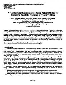
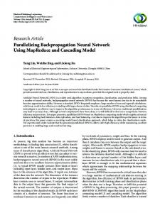
Figure 1. Speedup of Node Parallel as the neural network size increases (Data Set Size 10,000)
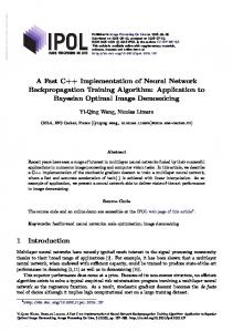
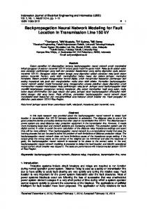
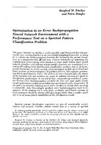
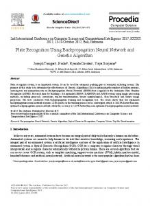
7 Performance Results For both strategies, the dominant factor in the performance is the dimension of parallelization. The node parallel implementation exhibits a strong correlation between performance and the size of the neural network. As shown in Figure 1, for a given dataset size (i.e. 10,000) the speedup grows steadily with the increased size of the network, with the best speedup 5.99 on 16 processors. For the tested range of neural network sizes (e.g. up to 16,000 with the data set size 100) the speedup of the node parallel version keeps growing steadily and has reached up to 16.36 on 32 processors, as shown in Figure 2. For this test only, the neural network size was increased to 4000, 8000 and 16,000. However, the experimental results show only a very weak correlation between performance and dataset size. Figure 3 shows, for a given size of the network (i.e. 2,000), the speedups are almost the same for different dataset sizes such as 1,000 and 10,000, though there is a slight trend for
Figure 2. Speedup of Node Parallel as the neural network size increases (Data Set Size 100)
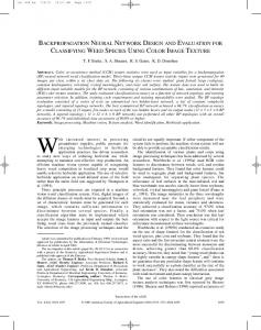
the speedup to drop on 32 processors when the dataset size grows to 10,000. The exemplar parallel implementation exhibits a strong correlation between performance and the size of the dataset. As shown in Figure 4, for a given network size (i.e. 1,000), the speedup grows quickly with the increased dataset size, with the best speedup of 16.66 on 32 processors. However, Figure 5 shows there is a relatively weak
the benefit due to the parallelization of the computation, and thus the speedup starts to drop.
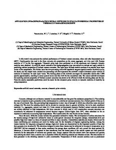
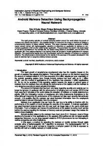
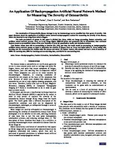
Figure 3. Speedup of Node Parallel as the data set size increases (Network Size 2,000) Figure 5. Speedup of Exemplar Parallel as the neural network size increases (Data Set Size 10,000)
Figure 4. Speedup of Exemplar Parallel as the data set size increases (Network Size 1,000)
correlation between performance and network size for a given dataset size (i.e. 10,000). In Figure 5, the speedup starts to drop on 32 processors when network size grows to 2000. The reasons are that the size of the data set determines the amount of computation done by each process for an epoch, while the size of the network determines the amount of data that must be sent. Therefore the larger the data set the higher the ratio between the computation and the communication, and thus the higher the speedup. When the network size grows to some point, say 2000, the communication overhead becomes large enough to overshadow
From our experimental results, we also notice that the impact of network size is greater on the exemplar parallel implementation, than the impact of the dataset size is on the node parallel implementation. As we mentioned, the exemplar parallel method appears to perform slightly worse on the neural network size 2,000 than the size 1,000. This is in general expected as the neural network size determines how much communication traffic occurs between processes. With the node parallel method, the size of the dataset determines the amount of network traffic and its communications load is more evenly distributed, i.e., it deals much better with increasing dataset sizes. The worst case performance for node parallelism is when the network size is very small, say 250, while for exemplar parallelism the worst case performance is when the dataset size is very small, say 100. In those cases, both applications exhibit a significant slowdown as the number of processors increases. Increasing the network size beyond the range of tested sizes, for a given data set size, should provide increasingly better performance for the node parallel strategy. Likewise, increasing the dataset size beyond the range of tested sizes, for a given network size, should provide increasingly better performance for the exemplar parallel strategy. However, in our experiments, we found that when the dataset size reaches beyond 40,000, the speedup stops growing at about 24 on 32 processors. Figures 6 shows the comparative performance of both strategies on 16 processors. Negative values (-1) show where the node parallel strategy provided the best performance, while positive values (1) show where the exemplar
parallel strategy performed best. When the size of the network is not very large, speedups of the exemplar parallelism tend to be better. When the size of the network is very large, the node parallelism tends to be better. We also calculated the theoretical costs of the two strategies based on equations 4 and 7. In our calculations, .�� .�
the values of � � ����� and ���� �� are �� � � %�� and %�� %� � %�� as determined by our cluster. Figure 7 shows the calculated costs. Negative values (-1) show where the node parallel strategy has the smaller cost, while positive values (1) show where the exemplar parallel strategy has the smaller cost. By comparing Figures 6 and 7, we know the theoretical comparison is very consistent with the experimental comparison, which shows we can use our theoretical cost equations to predict which strategy is going to be better given a network size and a dataset size, and thus choose that strategy for better performance. Figure 7. Comparison of theoretical cost with 16 processors
due to the node parallel strategy having a regular communications load which deals better with the increase in the size of the neural network. The choice of which strategy to use will be driven primarily by the type of learning required. If the problem requires on-line learning, node parallelism is the best option available. Otherwise for small dataset or for very large networks, the node parallel strategy tends to outperform exemplar parallelism. With large datasets, the exemplar parallel strategy will generally outperform node parallelism, particularly with smaller network sizes. Figure 6. Comparison of speedup performance on 16 processors
References [1] S. Haykin, Neural Networks: A Comprehensive Foundation (New Jersey: Prentice Hall, 1994).
8 Conclusion In this paper, we derived theoretical equations to determine the cost of two parallelization strategies for backpropagation neural networks. The two strategies were implemented and performance tests done. The actual results closely match the results predicted by the cost equations. As expected, both implementations performed well with the variation in the dimension of parallelization. Overall, for the test carried out, the exemplar parallel strategy generally outperformed the node parallel strategy, except for small datasets. The node parallel strategy is less susceptible to changes in the size of the dataset than the exemplar parallel strategy is to increases in the size of the network. This is
[2] T. Nordstrom and B. Svensson, Using and designing massively parallel computers for artificial neural networks, Journal of Parallel and Distributed Computing, 14(3), 1992, 260–285. [3] D. Rumelhart, G. Hinton, and R. Williams, Learning internal representations by error backpropagation, in D. Rumelhart, J. McClelland and The PDP Research Group (Ed.) Parallel Distributed Processing: Explorations into the Microstructure of Cognition, 1 (Cambridge: The MIT Press, 1986) 318–362. [4] M. Quoy, S. Moga, P. Gaussier, and A. Revel, Parallelization of neural networks using PVM, in Lecture Notes in Computer Science, 1908 (Berlin: Springer Verlag, 2000) 289–303.
[5] M. Misra, Parallel environments for implementing neural networks, Neural Computing Surveys, 1, 1997, 48–60. [6] U. Seiffert, Artificial neural networks on massively parallel computer hardware, Proceedings of the European Symposium on Artificial Neural Networks (ESANN’2002), Belgium, 2002, 319–330. [7] N. B. Serbedzija, Simulating artifical neural networks on parallel archectures, IEEE Computer, 29(3), 1996, 56–63. [8] B. Wilkinson and M. Allen, Parallel Programming (New Jersey: Prentice Hall, 1999). [9] A. Barak, O. La’adan, and A. Shiloh, Scalable cluster computing with MOSIX for Linux, Proceedings of the Linux Expo ’99, London, 1999, 95–100. [10] R. Rogers and D. Skillicorn, Strategies for parallelizing supervised and unsupervised learning in artificial neural networks using the BSP cost model, (Queens University, Kingston, Ontario, Canada, Tech. Rep., 1997). [11] Message Passing Interface Forum, MPI: A Message Passing Interface Standard, ( University of Tennessee, Knoxville, Tennessee, USA, Tech. Rep., 1994). [12] C. Lawson, R. Hanson, D. Kincaid, and F. Krogh, Basic linear algebra subprograms for FORTRAN usage, ACM Transactions on Mathematical Software, 5(3), 1979, 308–323. [13] J. Dongarra, J. D. Croz, S. Hammarling, and R. Hanson, An extended set of FORTRAN basic linear algebra subprograms, ACM Transactions on Mathematical Software, 14(1), 1988, 1–17. [14] D. Lay, Linear Algebra and Its Applications, 2rd ed. (Boston: Addison-Wesley, 2000).