Parameter Estimation for Blind and Non-Blind Deblurring Using ...

IEEE TRANSACTIONS ON IMAGE PROCESSING, 2013 (TO APPEAR)

1

Parameter Estimation for Blind and Non-Blind Deblurring Using Residual Whiteness Measures Mariana S. C. Almeida

and

M´ario A. T. Figueiredo, Fellow, IEEE

Abstract—Image deblurring (ID) is an ill-posed problem typically addressed by using regularization, or prior knowledge, on the unknown image (and also on the blur operator, in the blind case). ID is often formulated as an optimization problem, where the objective function includes a data term encouraging the estimated image (and blur, in blind ID) to explain well the observed data (typically, the squared norm of a residual) plus a regularizer that penalizes solutions deemed undesirable. The performance of this approach dependes critically (among other things) on the relative weight of the regularizer (the regularization parameter) and on the number of iterations of the algorithm used to address the optimization problem. In this paper, we propose new criteria for adjusting the regularization parameter and/or the number of iterations of ID algorithms. The rationale is that if the recovered image (and blur, in blind ID) are well estimated, the residual image is spectrally white; contrarily, a poorly deblurred image typically exhibits structured artifacts (e.g., ringing, oversmoothness), yielding residuals that are not spectrally white. The proposed criterion is particularly well suited to a recent blind ID algorithm that uses continuation, i.e., slowly decreases the regularization parameter along the iterations; in this case, choosing this parameter and deciding when to stop are one and the same thing. Our experiments show that the proposed whiteness-based criteria yield improvements in SNR, on average, only 0.15dB below those obtained by (clairvoyantly) stopping the algorithm at the best SNR. We also illustrate the proposed criteria on non-blind ID, reporting results that are competitive with state-of-the-art criteria (such as Monte-Carlobased GSURE and projected SURE), which, however, are not applicable for blind ID. Index Terms—Image deconvolution/deblurring, blind deblurring, whiteness, stopping criteria, regularization parameter.

I. I NTRODUCTION Image deblurring (ID) is an inverse problem where the observed image is modeled as the convolution of a sharp image with a blur filter, possibly plus some noise (often assumed spectrally white and Gaussian). With applications in many areas (e.g., astronomy, photography, surveillance, remote sensing, medical imaging), research on ID can be divided into non-blind ID (NBID), in which the blur filter is assumed c 2013 IEEE. Personal use of this material is permitted. Copyright ⃝ However, permission to use this material for any other purposes must be obtained from the IEEE by sending a request to [email protected]. Both authors are with the Instituto de Telecomunicac¸o˜ es, Instituto Superior T´ecnico, 1049-001 Lisboa, Portugal. M. Almeida is also with the ISCTE-Instituto Universit´ario de Lisboa, 1649-026 Lisboa, Portugal. Email: {mariana.almeida,mario.figueiredo}@lx.it.pt This work was partially supported by Fundac¸a˜ o para a Ciˆencia e Tecnologia (FCT), under grants PTDC/EEA-TEL/104515/2008, PEstOE/EEI/LA0008/2011, PTDC/EEI-PRO/1470/2012, and the fellowship SFRH/BPD/69344/2010. An earlier and shorter version of this work was published in [4].

known, and (more realistic) blind ID (BID), in which both the image and the blur filter are (totally or partially) unknown. Despite its narrower applicability, NBID is already a challenging problem to which a large amount of research has been (and still is) devoted, mainly due to the ill-conditioned nature of the blur operator: the observed image does not uniquely and stably determine the underlying original image [38]. If this problem is serious with a known blur, it is much worse if there is even a slight mismatch between the assumed blur and the true one. Most of the NBID methods overcome this difficulty through the use of an image regularizer, or prior, the weight of which has to be tuned or adapted [8], [13], [14], [15], [25], [28], [42], [51], [53]. Most state-of-the-art regularizers exploit the sparsity1 of the high frequency/edge components of images; this is the rationale underlying wavelet/frame-based methods (see, e.g., [21], [48] and the many references therein) and total variation (TV) regularization [42], [44]. With application not only in ID, but also in other inverse problems, several optimization techniques have been proposed to handle sparsity-inducing regularizers. A popular class of such techniques belongs to the class of iterative shrinkage/thresholding (IST) algorithms [22], [25], and their recent accelerated versions [7], [8], [56]. The iterative nature of these methods requires, in addition to the regularization parameter, the choice of an adequate stopping criterion; often, there is a delicate interplay between these two choices. In BID, even if the blur operator was not ill-conditioned, the problem would still be inherently ill-posed, since there is an infinite number of solutions (pairs of image and blur estimates) compatible with the blurred image. In order to obtain reasonable results, most BID methods restrict the class of blur filters, either in a hard way, through the use of parametric models [11], [12], [33], [43], [58], or in a soft way, through the use of priors/regularizers [5], [6], [24], [32], [34], [35], [40], [41], [47], [55]. In contrast, a recent BID method [3] does not use prior knowledge about the blur, yet achieves stateof-the-art performance on a wide range of synthetic and real problems. That method is iterative and starts by estimating the main features of the image, using a large regularization weight, and gradually learns the image and filter details, by slowly decreasing the regularization parameter. From an optimization point of view, this can be seen as a continuation method designed to obtain a good local minimum of the underlying non-convex objective function. The drawback of the method is that it requires manual stopping, which corresponds to 1 The term “sparse” is used here in a broad sense, meaning both actual sparseness (many zeros) or following a probability distribution concentrated near the origin and with heavy tails.

IEEE TRANSACTIONS ON IMAGE PROCESSING, 2013 (TO APPEAR)

choosing the final value of the regularization parameter. In fact, adjusting the regularization parameter and/or finding robust stopping criteria for iterative (blind or not) ID algorithms is a long standing, but still open, research area [15], [28], [42]. A crucial issue in the regularization of ill-posed inverse problems is the choice of the regularization parameter, a subject to which much work has been devoted [53]. The discrepancy principle (DP) [52] chooses the regularization parameter so that the variance of the residual (i.e., the difference between the observed image and the blurred estimate) equals that of the noise; the DP thus requires an accurate estimate of the noise variance and is known to yield over-regularized estimates [28]. A recent extension of the DP uses not only the variance, but also other residual moments [17]. Local residual statistics have also been used to obtain locally adaptive TV regularizers for NBID [19], [31]. Two other popular criteria are generalized cross validation (GCV) and the L-curve [29], [30], [52], which, although developed and mainly applied to linear methods, can also be used with non-linear methods, but are outperformed by more recent criteria based on Stein’s unbiased risk estimate (SURE) [23], [28], [36], [37], [45], [46], [54]. SURE provides an estimate of the mean squared error (MSE), assuming knowledge of the noise distribution and requiring an accurate estimate of its variance [59]. While methods for automatically adjusting the regularization parameter are relatively developed for denoising and NBID (as reviewed in the previous paragraph), the same is not true for BID, with most existing methods requiring the regularization parameters to be somehow tuned or empirically selected. For example, SURE-based approaches assume full knowledge of the degradation model, thus are not suitable for BID. There are a few methods that address the adjustment of the regularization parameter [5], [6], [24]; however, some of those approaches [6], [24] were developed for Bayesian formulations [5], [15], [27], [42], [52], and do not fit iterative BID algorithms such as that of [3]. Finally, we should mention no-reference image quality measures; although proposed for adjusting the regularization parameter in denoising [59], they can in principle be used in NBID or BID methods. A. Contributions We propose a criterion that can be used to adjust the regularization parameter and stopping criterion of iterative ID methods; although motivated by BID problems, it is of general applicability to both NBID and BID problems. The cornerstone of the proposed approach is the assumption that the noise in the observed image is spectrally white. The implementation of this rationale is based on measures of spectral whiteness to assess the fitness of the current estimates to the degradation model. Residual whiteness has been used for a long time to assess model accuracy, namely in modeling time series and dynamical systems [9], [39]; more recent applications can be found in spectroscopy [18] and signal detection [50]. However, to the best of our knowledge, criteria based on residual whiteness have not been used before in image deconvolution/deblurring. Our criteria are particularly suited to the BID method of [3], where stopping and choosing the regularization parameter

2

are one and the same thing. The results reported in this paper, show that, on a large set of synthetic experiments, the proposed criteria lead to an average decrease of 0.15 dB in ISNR2 , compared to what is obtained by stopping the algorithm at the maximum ISNR (which, of course, cannot be done in practice, as it requires the original image), outperforming in this sense both the DP and the measure of [59]. We also show tests on color images and on various real blurred images; although with these images, no quantitative results can be reported, we believe the results can be (subjectively) considered good. We show that the proposed criteria are also suitable for adjusting the regularization parameter and stopping criterion of NBID methods. In particular, we report experiments with two recent algorithms, using different blurs and noise variances. In this scenario, our approach is shown to be adequate, but does not outperform SURE-based methods. B. Outline The remaining sections of this paper are organized as follows. The formulation of blind and non-blind ID is briefly reviewed in Section II and the proposed criteria are described in Section III. Section IV reports experiments on both nonblind and blind settings, and Section V concludes the paper. II. I MAGE D ECONVOLUTION /D EBLURRING In ID problems, the degraded image is usually modeled as y = h ∗ x + n,

(1)

where y is the degraded image, x is the (unknown) original image, n is noise, and h is the point spread function (PSF) of the blur operator (assumed to be known in NBID and unknown in BID) and ∗ denotes convolution. Both BID (finding x and h, from y) and NBID (finding x, from y and h) are normally addressed by adopting a regularizer expressing prior information about the image x and considering an objective function of the form 1 2 ∥y − h ∗ x∥2 + λ Φ(x); (2) 2 the first term in (2) is the classical data fidelity term that results from assuming that the noise n is white and Gaussian, Φ(x) is a regularization function embodying the prior information about x, and λ is the regularization parameter. Typically, too large values of λ lead to over-regularized images (e.g., oversmoothed or cartoon-like), while too small values of λ lead to under-regularized images dominated by the influence of the noise. An adequate choice of the regularization parameter λ is thus clearly crucial to obtain a good image estimate. Cλ (x, h) =

A. Non-blind Deblurring In NBID, h is assumed to be known and the cost function (2) is minimized with respect to x, given some choice of the regularization parameter λ. Many optimization methods for ID minimize the cost function (2) iteratively [7], [8], [22], [25], [56], computing the image estimate at iteration t + 1 as a 2 ISNR

denotes improvement in signal-to-noise ratio.

IEEE TRANSACTIONS ON IMAGE PROCESSING, 2013 (TO APPEAR)

3

function of the previous estimate xt , the available data (y and h), and the regularization parameter λ: xk+1 = f (xk , y, h, λ).

(3)

Algorithm 1: Blind method of [2], [3] 1 2 3

Besides requiring a good estimate for the regularization parameter λ, these iterative approaches also need stopping criteria, which considerably influence the final results. For fairness, it should be mentioned that some state-of-theart methods don’t fall in the category of methods mentioned in the previous paragraph. For example, the method proposed in [16] (arguably the method yielding the current best results) is iterative, but rather than look for a minimizer of an objective function, it looks for a Nash equilibrium between two objective functions. Other NBID methods are not based on iterative minimization of objective functions [51], [57] B. Blind Deblurring In BID, both the image x and the filter h are unknown. A BID problem suffers from an obvious lack of data, since there are many pairs (x, h) that explain equally well the observed data y. Most BID methods circumvent this difficulty by adding to (2) a regularizer on the blur filter and, usually, by alternatingly estimating the image and the blur filter. A regularizer on the blur naturally involves an additional regularization parameter, also requiring adjustment, while the alternating estimation of the image and the filter requires good initialization (since the underlying objective (2) is non-convex) and a good criterion to stop the iterative process. The recent method in [2], [3] yields good results without regularization on the blur filter, i.e., using a cost function with the form of (2). That method uses an iterative algorithm to minimize (2), by starting with a strong regularization (large λ), and gradually decreasing it (see Algorithm 1). The initial estimates are cartoon-like; the sharp edges of these images, when compared with the blurred image y, allow to learn and improve the estimate of the filter h, which, in turn, allows reducing the weight of the regularization, thus learning finer image details. This slow decrease of the regularization parameter was shown to yield good estimates without the need for a regularizer on the blur filter [3]. A drawback of that method is the need to manually stop the iterations, which corresponds to setting the final value of the regularization parameter. In [3], this was done either based on the ISNR value, in synthetic experiments, or by visual assessment of the restored image, for real blurred images. The whitenessbased criteria proposed in this paper will be illustrated in automatically stopping the BID algorithm of [3]. III. T HE W HITENESS C RITERIA A. Rationale The proposed criteria for selecting the regularization parameter and the stopping iteration are based on measures of the fitness of the image estimate x b and the blur estimate b h (in NBID, h is known, thus b h = h) to the degradation model (1), by analyzing the estimated residual image: r = y−b h∗x b.

(4)

4 5 6 7

Set λ to the initial value; choose α < 1. Set x b=y repeat b h ← arg minh Cλ (b x, h) x b ← arg minx Cλ (x, b h) λ←αλ until stopping criterion is satisfied

The characteristics of the residual r are then compared with those assumed for the noise n in the degradation model (1). In particular, the noise n is assumed to be spectrally white (uncorrelated), thus a measure of the whiteness of the residual r is used to assess the adequacy of the estimates (b x,b h) to the model. This is a quite generic assumption, valid for most real situation. Our approach differs from other methods based on residual statistics, such as those in [17], [52], in that those methods do not use spectral properties of the residual, but other statistics, such as variance and other moments. The proposed criterion consists in selecting the regularization parameter and/or final iteration of the algorithm that maximize one of the whiteness measures introduced below. If this measure exhibits a clear peak as a function of the regularization parameter and/or the iteration number, we adopt an oriented search scheme and stop the method as soon as the measure of whiteness starts to decrease. This is the case in the BID algorithm mentioned in the previous section. Also in NBID, if optimizing only with respect to λ, an efficient strategy is to sweep a range of values, using the estimate at each value to initialize the algorithm at the next value; this process is known warm-starting, and may yield large computational savings [56]. In our NBID experiments, when optimizing with respect to λ and/or the number of iterations, and since the goal is to assess the ability of the proposed criteria to select these quantities, with no concern for computational efficiency, we simply consider a grid of values and return the image estimate yielding the maximum residual whiteness. B. Measures of Whiteness The first step of our method is to normalize the residual image3 to zero mean and unit variance; for simplicity of notation, let this normalized residual still be denoted as r, r−r r← √ , var(r) where r and var(r) are, respectively, the sample mean and sample variance of r. The auto-correlation (and autocovariance, since the mean is zero) of the normalized residual r, at the two-dimensional (2D) lag (m, n), is estimated by ∑ Rrr (m, n) = K r(i, j) r(i − m, j − n), (5) i,j 3 In our experiments, the convolution needed to obtain the residual (4) is computed using the FFT; a band of pixels at the residual image boundary is then discarded from the computation of the whiteness measures, to avoid the boundary artifacts caused by the FFT.

IEEE TRANSACTIONS ON IMAGE PROCESSING, 2013 (TO APPEAR)

4

where the sum is over the residual image, and K is an irrelevant constant. The auto-covariance of a spectrally white image is a delta function at the origin (δ(m, n) = 1, if m = n = 0, δ(m, n) = 0, otherwise). A measure of whiteness is thus the distance between Rrr and a delta function. Considering a (2L + 1) × (2L + 1) window, the first proposed whiteness measure is simply the energy of Rrr outside the origin, (

L,L ∑

MR (r) = −

)2 Rrr (m, n) ,

(6) D. Color Images

(m,n)=(−L,−L) (m,n)̸=(0,0)

where the minus sign is used to make MR larger for whiter residuals. In our experiments, we have used L = 4. For a typical process that exhibits mainly short-range correlations, the auto-covariance for large lags (for long-range dependencies) is usually smaller than for small lags. This observation suggests that it makes sense to give more weight to the auto-covariance for small lags. Based on that, a weighted version of the measure in (6) is also considered, MRW (r) = −

L,L ∑

( )2 W (m, n) Rrr (m, n) , (7)

(m,n)=(−L,−L) (m,n)̸=(0,0)

where W (m, n) is a matrix of weights. In all our experiments, we have used L = 4 and the gausswin function in MATLAB: ( ) W (m, n) = exp −1.25(m2 + n2 ) . (8) Let Srr (ω, ν) denote the power spectral density of r, at 2D spatial frequency (ω, ν), Srr = F(Rrr ),

partially overlapping 9 × 9 blocks, separated horizontally and vertically by 5 pixels, and only those that are fully contained in the image domain. Of course, in this case, the residual is normalized to zero mean and unit variance on a block-byblock fashion, rather than globally. Given this block partition, l l the three local measures of whiteness, MRl , MRW and MH are obtained by computing the corresponding local measures MR , MRW , and MH , respectively, at each block, and then averaging over all the blocks of the image.

The measures of whiteness presented in the previous subsection were defined for gray-scale images. In order to use them with color images, several approaches can be followed. Assuming that the three color channels were degraded by the same blur filter, we adopt a simple procedure in all the examples reported below. At each iteration of Algorithm 1, the image estimate is converted to gray-scale and the residual is computed using a (previously computed) gray-scale version of the blurred image and the current blur filter estimate. In the NBID case (although we don’t report any experiments), the degraded and the estimated images are converted to gray scale, where the proposed whiteness measures are computed. IV. E XPERIMENTS In this section, we experimentally compare the proposed criteria with several state-of-the-art techniques. Since our proposal was motivated by BID problems, we report more experiments in that scenario, for which fewer methods are available. Finally, we also report some NBID experiments, showing that proposed criteria also work for NBID.

(9)

where F denotes the magnitude of the 2D discrete Fourier transform (2D-DFT). Since the auto-correlation of a white process is a delta function, a white signal has a flat power spectral density. To assess the flatness of Srr , we measure its Shannon entropy, after normalization; recall that the maximum entropy is achieved by a flat distribution. The resulting measure is ∑ MH (r) = − Serr (ω, ν) log Serr (ω, ν), (10) ω,ν

∑ where Serr (ω, ν) = Srr (ω, ν)/ ω′ ,ν ′ Srr (ω ′ , ν ′ ). C. Local Measures of Whiteness The approach described in the previous subsection implicitly assumes that the residual image r is a sample of a stationary and ergodic process, since we estimate the auto-covariance (5) by averaging over the whole image. In practice, the residual may not be stationary, which lead us to consider also local versions of the previous measures of whiteness, based on local auto-covariance estimates, ∑ b r(i, j) r(i − m, j − n), (11) Rrr (m, n) = i,j∈Bb

where b indexes an image block, and Bb is the set of pixels in that block. In the experiments reported below, we have used

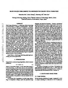
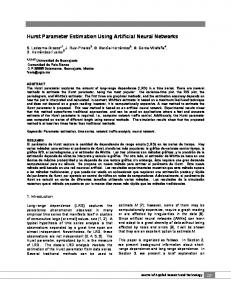
A. Blind deblurring This subsection demonstrates the effectiveness of the proposed criteria in stopping (which in this case coincides with selecting the regularization parameter) a state-of-the-art BID method [3]. Note that most existing methods for regularization parameter selection (namely SURE) are not adequate for the blind case. 1) Synthetic experiments: We consider most of the experiments described in [3]: (i) four benchmark images (Lena, Barbara, Cameraman, and Satellite); (ii) seven different blurs (see Fig. 1); (iii) addition or not of Gaussian white noise, with BSNR (blurred-signal-to-noise-ratio) of 30dB; (iv) experiments with and without constraints4 on the blur filter. We ran BID experiments using (almost5 ) all possible combinations (totalling 96) of images, blurs, and presence/absence of constraints and noise (as described in the previous paragraph), and all the whiteness measures described in Section III. Before reporting detailed experiments, Fig. 2 illustrates the behavior of one of the proposed criteria (MRl , in this example), by showing how its evolution correlates well with that of the 4 Blur constraints (see Fig. 1): (a) is parameterized as a circle with the radius as the estimated parameter; (b) is constrained to be symmetric around the origin; (c)–(e) are constrained to having reflection symmetry around the horizontal and vertical axes and 45o rotations thereof. 5 No simple symmetry constraints are available for blurs (f) and (g).

IEEE TRANSACTIONS ON IMAGE PROCESSING, 2013 (TO APPEAR)

5

bottom rows indicate that the criterion is more suitable when there is no access to extra information on the blur filter. (a)

(b)

(c)

(d)

(e)

(f)

(g)

Fig. 1. Blur kernels for the synthetic experiments: (a) out-of-focus, (b) linear motion, (c) uniform square, (d) Gaussian, (e)–(f) nonlinear motions, (g) random.

ISNR, along the iterations (thus also as a function of the regularization parameter). Clearly, for too high (early iterations) or too low (later iterations) values of the regularization parameter, the residual images exhibit structures which are far from being spectrally white. At the best ISNR, the residual image has little structure, thus being approximately spectrally white, thus the auto-covariance estimate Rrr is essentially a delta function. Table I summarizes the average results6 (over the 96 experiments) obtained using the proposed stopping criteria. It is clear that all the criteria are able to stop the algorithm at estimates which are, on average, only slightly worse than the best ISNR achieved along the iterations of the algorithm. However, it l , MRl , and is clear that the local whiteness measures (MH l MRW ) achieve better results than their global versions. The results are also reasonably stable, as shown by the standard deviation of the ISNR decrease, which are clearly below 1dB. This can be considered as a successful result, considering the wide set of degradations that were considered and the wellknown difficulty of BID problems. TABLE I AVERAGE PERFORMANCE OF THE SIX CRITERIA ( IN dB), IN TERMS OF THE DIFFERENCES ( DENOTED ∆ISNR) BETWEEN THE ISNR OBTAINED BY STOPPING WITH EACH OF THE AUTOMATIC CRITERIA AND THE BEST ISNR ACHIEVED ALONG THE ALGORITHM .

REPORTS DIFFERENCE IN ITERATION COUNT BETWEEN THE OCCURRENCE l AND THAT OF ISNR. OF THE MAXIMUM OF MR

All noiseless noisy constrained unconstrained

MH

MR

MRW

l MH

best ISNR 5.88 dB 6.90 dB 4.85 dB 6.60 dB 5.36 dB

∆ISNR mean -0.15 dB -0.20 dB -0.09 dB -0.21 dB -0.10 dB

l MRW

Mean

5,88

-0.38

-0.40

-0.37

-0.16

-0.15

-0.16

St. dev.

2,63

0.62

0.62

0.70

0.29

0.27

0.30

Table II shows more details about the results obtained with the local measure MRl (the best performing one, according to Table I). The results in the rightmost column of Table II show that the maxima of MRl tend to occur somewhat earlier than those of the ISNR. The results also suggest that these iteration differences are larger in the absence of added noise; however, in this case, the ISNR reaches a plateau, thus this premature stopping does not imply a large degradation in ISNR. One may raise the question of why the residual whiteness criterion still works in the absence of added noise. In fact, even if no noise is added, there are always residuals, because deconvolution is an ill-posed problem that is being addressed under regularization; if this residual has some spatial structure (is non-white), that means that it contains some information about the underlying image and filter that could be used to improve the restoration accuracy. Finally, the two 6 These values are slightly different from those in [4]; there, the residual at each iteration is computed using the blur estimated from the image at that iteration (used to obtain the next image estimate), whereas here we use the previous blur estimate (used to estimate the image at the present iteration).

∆Iter. mean -6.3 -11.9 -0.7 -8.0 -5.1

TABLE III l WITH TWO VERSIONS C OMPARISON ( IN TERMS OF ∆ISNR, IN dB) OF MR OF THE DISCREPANCY PRINCIPLE (DP σ AND DP MAD , SEE TEXT ) AND THE NO - REFERENCE MEASURE (NR) OF [59].

∆ISNR

ISNR l MR

∆ISNR st. dev. 0.27 dB 0.34 dB 0.11 dB 0.16 dB 0.33 dB

2) Comparison with Other Criteria: In this section we compare our best criterion, MRl , against the discrepancy principle (DP) and the no-reference measure from [59]. Since the DP requires knowledge of the noise variance, we consider two variants: one that uses the true value of the added noise, referred to as DPσ , and another one that uses an estimate of the noise obtained by the well-known MAD (mean absolute derivative) rule [20]. The results in Table III show that, with the single exception of the noiseless case, where DPσ obtains the best result, MRl yields less loss of ISNR than the other methods. Notice that DPσ cannot be used in practice, as it requires the true value of the noise variance.

∆ISNR

ISNR Best

TABLE II l IN DIFFERENT CLASSES OF B REAK UP OF THE RESULTS OF MR EXPERIMENTS (∆ISNR IS AS DEFINED IN TABLE I). T HE LAST COLUMN

All noiseless noisy constrained unconstrained

best 5.88 6.90 4.85 6.60 5.36

l MR

-0.15 -0.20 -0.09 -0.21 -0.10

DPσ -0.22 -0.09 -0.35 -0.29 -0.17

DPMAD -1.95 -2.59 -1,31 -2.36 - 1.65

NR -2.80 -2.92 -2.68 -3.09 -2.60

3) Application to Real Blurred Photos: We now test the proposed stopping criteria on several real-life (both color and monochrome) blurred photos (with out-of-focus or motion blurs, as shown in Fig. 3). Three of these images were used in [3] ((c), (d), and (e)), two ((f) and (g)) were downloaded form the URL of the paper [32] (http://cs.nyu.edu/∼dilip/research/blind-deconvolution/), and two are new ((a) and (b)). Table IV shows, for each degraded photo, the iteration numbers that were automatically selected with the proposed criteria and the “optimal” iteration that was selected based on the authors’ visual assessment. The iterations manually and automatically selected are close, showing that the proposed criteria are suitable for real-life scenarios. In all these experiments, our criteria always select image estimates that are quite similar to those corresponding to the “best” results. For a visual evaluation of these results, Figs. 4–6 show some image and filter estimates at the iterations

IEEE TRANSACTIONS ON IMAGE PROCESSING, 2013 (TO APPEAR)

6

Fig. 2. Illustration of the proposed approach; results obtained with the Lena image, blurred with an out-of-focus blur and contaminated with noise at 30dB BSNR. Evolution along the iterations (from top to bottom) of: Rrr , residual image r, whiteness measure MR , and ISN R.

corresponding to the maximum value of MRl and to the “best” visual quality. B. Non-blind Deblurring The goal of this subsection is to test the proposed criteria for NBID. For that purpose, we used two recent algorithms: SpaRSA7 (sparse reconstruction by separable approximation) [56], which is a recent fast algorithm of the IST family, and (following a suggestion by one of the reviewers) SALSA8 (split augmented Lagrangian shrinkage algorithm) [1], which is an instance of the alternating direction method of multipliers (ADMM) [10], [26]. Notice that the choice of these algorithms is somewhat arbitrary, since the proposed criteria can be applied to any iterative deconvolution algorithm that has a regularization parameter and/or a stopping criterion; for this reason, we decided not to include any details about those algorithms and refer the reader to [1], [56], for more details. Whereas in BID, the local measures were shown to perform somewhat better the global ones, preliminary experiments showed that in NBID the differences are very small, so we considered only the global measures, since they are computationally less demanding. All our NBID experiments were run on the standard Cameraman image (with pixel values in [0, 255]), with the blurs and noise levels shown in Table V). In order to determine the regularization parameter and the stopping iteration for SpaRSA, the algorithm is run for up to 151 iterations, using a geometric sequence of 21 values of 7 Available 8 Available

online at http://www.lx.it.pt/∼mtf/SpaRSA/ online at http://cascais.lx.it.pt/∼mafonso/salsa.html

TABLE V D IFFERENT EXPERIMENTAL SETTINGS FOR THE NBID EXPERIMENTS . T HE COLUMN “ CONDITION ” SHOWS THE CONDITION NUMBER OF THE BLUR FILTER IN THE FREQUENCY DOMAIN ( BLURS NORMALIZED TO UNIT 2 DC GAIN ). T HE COLUMN σM AD SHOWS NOISE VARIANCE ESTIMATE GIVEN BY THE MAD RULE .

Exp.

blur kernel h(m, n)

σ2

condition

2 σMAD

1 2

Gaussian (stdv = 0.5) h = [1 4 8 4 1] (horizontal blur) Gaussian (stdv = 0.7)

5 5

3.033 9

6.221 5.332

5

31.5

5.224

(1 + m2 + n2 )−1 −4 < m, n < 4 (1 + m2 + n2 )−1 −4 < m, n < 4 9 × 9 uniform

2

67.1

2.082

8

67.1

6.377

0.3136

2.2×105

0.535

7

3 4 5 6 7

Gaussian (stdv = 2)

2

2.3×10

4.131

8

T

2

∞

2.278

[1 4 6 4 1] [1 4 6 4 1] (separable blur)

the regularization parameter: from λ1 = 0.035 × (1.5)−10 ≈ 6 × 10−4 , up to λ21 = 0.035 × (1.5)10 ≈ 2. For each of the 151 × 21 image estimates, the several measures being compared are computed and the final image estimates (and the corresponding parameters) are those yielding their maxima. Table VI reports the ISNR values thus obtained by our three global criteria, the three criteria considered for the blind case (DPσ , DPMAD , NR), as well as the P-GSURE and PD-GSURE:

IEEE TRANSACTIONS ON IMAGE PROCESSING, 2013 (TO APPEAR)

7

a) “Studio-motion”, 256×256.

b) “Studio-blur”, 256×256.

c) “Building”, 256×256.

d) “House-blur”, 256×256.

e) “House-motion”, 256×256.

f) “Mukta”, 610×406, (from [32]).

g) “Pietro”, 636×848, (from [32]). Fig. 3.

Real-life photos used in the experiments. (b), (c), and (d) are out of focus; (a), (e), (f), and (g) suffered motion blur.

two recent state-of-the-art criteria (reviewed in the Appendix) [23]. Both P-GSURE and PD-GSURE were implemented using the Monte-Carlo divergence estimate proposed in [45] (also briefly reviewed in the Appendix). One disadvantage of SURE-based measures is that they require knowing the noise variance σ 2 ; similarly to what was done for the DP, we considered two options: using the true noise variance ( P-GSUREσ and PD-GSUREσ ) and its MAD estimated (P-GSUREMAD and PD-GSUREMAD ). The results presented in Table VI the whiteness-based criteria perform adequately; although our measures are only the best for one experimental setting, they are not very far. A conclusion that can also be drawn is that the no-reference method of [59], although it was proposed and tested only for denoising by its authors, does provide a good criterion also for NBID (in contrast with its comparatively poor performance in the BID scenario). Concerning SALSA, and since the stopping criteria for ADMM-based algorithms is more involved than for algorithms of the IST family, we have used the built-in stopping criterion with its default setting, and have used the proposed whiteness

measure only for adjusting the regularization parameter. The results shown in Table VII lead to the same general conclusions as for SpaRSA. For relatively well-posed problems (condition numbers up to around 30), the ISNR results obtained with the four SUREbased criteria typically outperform those obtained with MRW . This is not surprising, since SURE directly approximates the MSE. SURE-based measures, however, have the disadvantage of assuming an exact form for the distribution of the noise, leading to biased results when incorrect information is used [59]. On the other hand, the accuracy of the Monte-Carlo SURE-based measures deteriorates as the conditioned number gets worse. This is probably due to the computation of the divergence term (19), which becomes extremely sensitive to the sufficient statistic u (see (13)). The negative effect of the condition number in this GSURE estimate is visible in Fig. 7, which compares the some of the computed measures and the true MSE, along the 21 values of regularization parameter and the 151 iterations of SpaRSA. In contrast with Monte-Carlo SURE-based measures, the whiteness measure MRW always lead to good results, although slightly over-regularized with

IEEE TRANSACTIONS ON IMAGE PROCESSING, 2013 (TO APPEAR)

8

“Studio-motion”, visual criterion, 23rd iteration. “Studio-motion”, criterion based on MRl , 21st iteration.

“Studio-blur”, visual criterion, 22nd iteration.

“Studio-blur”, criterion based on MRl , 23rd iteration.

“Building”, visual criterion, 23rd iteration.

“Building”, criterion based on MRl , 23rd iteration.

Fig. 4. Results obtained with real blurred photos. From left to right, at each row: restored image at the “optimal” (visually selected) iteration, estimated blur l , blur filter estimate at the iteration chosen using M l . filter at the “optimal” iteration, restored image at the iteration chosen using MR R

respect to those at the highest ISNR value. Although yielding, in some experiments, ISNR values that may seem relatively low, the visual results reached with MRW were actually good, and not as poor as the quantitative measure may sometimes suggest; some of these results are shown in Fig. 8. V. C ONCLUSIONS We have proposed new criteria that can be used to select the regularization parameter and to stop iterative blind and non-blind image deconvolution algorithms. Our proposal is based on measures of the whiteness of the residual image. The approach is quite general and does not require any knowledge about the type of convolution operator. The proposed criteria were motivated by blind deconvolution problems, and it is particularly well suited to a recent state-of-the-art method that uses a continuation scheme based

on the regularization parameter. For that method, choosing the regularization parameter and deciding when to stop are one and the same thing. On a wide range of synthetic experiments, we showed that the best of the proposed criteria yields ISNR losses with the respect to the best ISNR of only 0.15dB, on average. The method was also compared with two other criteria, of the few that can be used in blind deconvolution problems, showing to perform better in terms of SNR. Finally, tests on several real photos, degraded with various out-of-focus and motion blurs, showed that the proposed method yields visually good results. The proposed approach was shown to be also adequate (although not achieving state-of-the-art results in terms of SNR) for estimating both the regularization parameter and the number of iteration of non-blind deblurring algorithm.

IEEE TRANSACTIONS ON IMAGE PROCESSING, 2013 (TO APPEAR)

9

“House-blur”, visual criterion, 22nd iteration.

“House-blur”, criterion based on MRl , 24th iteration.

“House-motion”, visual criterion, 23rd iteration.

“House-motion”, criterion based on MRl , 22nd iteration.

“Mukta”, visual criterion, 24th iteration.

“Mukta”, criterion based on MRl , 24th iteration.

Fig. 5. Results obtained with real blurred photos. From left to right, at each row: restored image at the “optimal” (visually selected) iteration, estimated blur l , blur filter estimate at the iteration chosen using M l . filter at the “optimal” iteration, restored image at the iteration chosen using MR R

A PPENDIX A. GSURE The well known SURE (Stein’s unbiased risk estimate) is an unbiased estimator of the MSE achieved by an (almost arbitrary) estimator of an unknown vector observed under additive white Gaussian noise [49]. SURE have been directly applied to tune the regularizing parameter of linear and nonlinear denoising methods [45], [37]. Recently, SURE was extended to observation models in the class of exponential family distributions [23]; this generalized SURE (GSURE) can be used for tuning the regularizing parameter in non-blind ID [23]. Consider the vectorial representation of (1) y = Hx + n

(12)

in which x ∈ Rm , y ∈ Rm and n ∈ Rm are vectors with the elements of x, y and n, respectively, in lexicographical order, and H ∈ Rm×m is the matrix representing the linear operation of the convolution with the filter h. Defining hλ (·) as the functional that, from the sufficient statistic of the model (12) (u = (1/σ 2 )HT y), returns the output of a deblurring method with a regularization parameter λ, the GSURE estimate of the MSE is given, up to a constant, by [28] 2

η(hλ (u), y) = ∥hλ (u)∥ − 2 xTML hλ (u) + 2 ∇u · hλ (u), (13) where xM L is the maximum likelihood (ML) estimator, and ∑ ∂hλ,i (u) (14) ∇u · hλ (u) = ∂ui i

IEEE TRANSACTIONS ON IMAGE PROCESSING, 2013 (TO APPEAR)

10

“Pietro”, visual criterion, 21th iteration.

“Pietro”, criterion based on MRl , 22th iteration.

Fig. 6. Results obtained with a real blurred photo. From left to right: restored image at the “optimal” (visually selected) iteration, estimated blur filter at the l , blur filter estimate at the iteration chosen using M l . “optimal” iteration, restored image at the iteration chosen using MR R TABLE IV C OMPARISON OF THE PROPOSED

STOPPING CRITERIA VERSUS THE VISUAL CRITERION ( DENOTED AS “ BEST ”); THE NUMBERS ARE THE ITERATIONS AT WHICH THE ALGORITHM WAS STOPPED BASED ON EACH OF THE CRITERIA .

“Studio-motion” “Studio-blur” “Building” (gray-scale) “House-motion” (gray-scale) “House-blur” (gray-scale) “Mukta” (gray-scale) “Pietro” (gray-scale) “Building” (color) “House-motion” (color) “House-blur” (color) “Mukta” (color) “Pietro” (color)

MH 19 22 25 26 26 24 24 24 23 26 23 22

MR 19 22 26 26 26 24 24 24 23 26 24 22

MRW 22 22 25 26 25 24 24 24 23 25 24 24

l MH 22 22 25 26 24 24 24 23 22 24 24 23

l MR 21 23 25 27 24 24 24 23 22 24 24 22

l MRW 23 22 25 26 24 24 24 23 23 24 24 23

“Best” 23 22 25 25 24 24 23 24 23 24 24 21

TABLE VI C OMPARISON OF THE PROPOSED GLOBAL CRITERIA VERSUS SEVERAL OTHER METHODS ( RESULTS ARE ISNR VALUES , IN dB) USING S PA RSA WITH THE REGULARIZATION PARAMETER AND STOPPING ITERATION SELECTED BY EACH CRITERION . S EE TEXT FOR DETAILS ABOUT THE COMPARED METHODS .

Best

1 4.91

2 23.95

MH MR MRW DPσ DPMAD NR P-GSURE P-GSUREMAD PD-GSURE PD-GSUREMAD

3.59 3.59 3.35 3.33 3.35 3.72 4.91 4.67 4.91 4.67

21.14 21.14 21.14 22.28 21.89 21.87 23.87 23.87 23.77 23.77

Experimental setting (see Table V) 3 4 5 6 7 4.59 5.77 3.87 6.77 2.35 3.10 2.94 3.08 2.47 2.45 3.59 4.59 4.49 4.49 4.49

denotes the divergence of hλ . For the case of non-invertible blurs, [23], [28] suggest estimating the MSE that lies on the range of HT , denoted as R(HT ). Considering PR(HT ) = HT (HHT )† H (where † denotes Moore-Penrose pseudo inverse), the orthogonal projection onto the range of HT , the GSURE estimate of the projected MSE, referred to as projected SURE (P-GSURE) is given, up to a constant, by

2 ηPR(HT ) (hλ (u), y) = PR(HT ) hλ (u) − 2 xM L · hλ (u) +2 ∇u · hλ (PR(HT ) u),

(15)

4.53 4.53 5.11 5.13 4.38 5.38 1.87 1.87 1.87 1.87

3.01 3.01 3.01 2.60 3.77 3.28 -9.25 -9.25 -7.35 -7.35

6.38 6.38 6.38 5.16 4.10 5.96 5.34 5.53 5.53 5.53

1.29 1.31 1.48 1.35 1.19 2.10 1.17 1.17 1.76 1.76

8 3.59 1.72 1.98 2.60 2.16 2.22 2.79 3.26 2.96 3.22 3.22

where xM L = HT (HHT )† y. An equivalent result was derived in [54] for non-blind ID, although limited to the case of invertible blurs. In the experiments reported in Tables VI and VII, the projected version is used with experimental settings 6, 7, and 8, which are the most ill-conditioned.

B. Predicted SURE The predicted SURE (PD-SURE) is a SURE-based unbiased estimator of the predicted-MSE (mean square error on the data

IEEE TRANSACTIONS ON IMAGE PROCESSING, 2013 (TO APPEAR)

11

TABLE VII C OMPARISON OF THE PROPOSED GLOBAL CRITERIA

VERSUS SEVERAL OTHER METHODS ( RESULTS ARE ISNR VALUES , IN dB) USING SALSA WITH THE REGULARIZATION PARAMETER SELECTED BY EACH CRITERION . S EE TEXT FOR DETAILS ABOUT THE COMPARED METHODS .

Best

1 5.64

2 6.34

MH MR MRW DPσ DPMAD NR P-GSURE P-GSUREMAD PD-GSURE PD-GSUREMAD

3.66 3.66 3.66 3.66 3.66 4.96 5.64 5.64 5.64 5.64

3.39 4.44 3.39 4.44 4.44 5.32 6.34 6.34 6.01 6.01

Experimental setting (see Table V) 3 4 5 6 7 5.78 7.09 5.11 8.61 3.11 4.20 4.20 4.40 4.20 4.20 4.99 5.78 5.58 5.58 5.58

6.10 6.10 6.10 6.10 6.10 6.10 7.09 7.09 7.09 7.09

4.33 4.33 3.74 4.33 5.11 3.19 5.11 0.69 5.11 4.61

7.60 8.09 7.60 8.09 5.89 8.09 8.09 7.03 8.61 8.09

2.70 2.86 2.70 2.70 0.88 -16.14 2.29 2.51 3.07 3.11

8 4.75 3.79 3.79 3.31 3.79 3.31 4.23 4.56 4.23 4.73 4.56

Fig. 7. Maps of different criteria (for experiment 5), along the 21 values regularization parameters (vertical axis) and the 151 iterations (horizontal axis). From left to right: MSE, GSUREMAD , NR, DPMAD , and log10 (−MRW ).

domain): 1 ||H(x − uλ (y))||22 , (16) m in which uλ () is the functional that computes the image estimate from the degraded image y. PD-SURE is given, apart from a constant, by [45]: Predicted-MSE(λ) =

1 ||y − Huλ (y))||22 + m 2σ 2 + tr {HJ(uλ , y)} (17) m where J(uλ , y) represents the Jacobian matrix of uλ evaluated at y, and the last term relates to the divergence of uλ () PD-SURE(λ) =

tr {HJ(uλ , y)} = ∇y · Huλ (y),

(18)

in which the divergence ∇y · Huλ (y) can be easily computed according to the next section. C. Monte-Carlo estimation of the divergence The difficulty in using SURE-based measures (SURE, GSURE or PD-SURE) resides in computation/approximating the divergence term, as it involves derivatives of a function defined via an optimization problem. To overcome this hurdle, [45] proposed a Monte-Carlo method to estimate the divergence of a function g by treating it as a black-box: 1 T b (g(z + ϵ b) − g(z)), (19) ϵ where b is a zero-mean random vector of unit variance and ϵ is a small positive parameter. Implementing this divergence estimator only requires applying the estimator g twice, to the input z and to a perturbed version thereof. Parameter ϵ should ∇z · g(z) ≃

be small for an accurate estimate of the divergence, but large enough to avoid numerical errors. For all the experiments, the Monte-Carlo divergence estimate of (14) and (18) were computed as in (19), with ϵ = 0.01. R EFERENCES [1] M. Afonso, J. Bioucas-Dias, and M. Figueiredo, “Fast image recovery using variable splitting and constrained optimization,” IEEE Trans. Image Processing, vol. 19, pp. 2345–2356, 2010. [2] M. S. C. Almeida and L. B. Almeida, “Blind deblurring of natural images,” in IEEE Int. Conf. Acoustics, Speech, and Signal Processing ICASSP, 2008, pp. 1261–1264. [3] ——, “Blind and semi-blind deblurring of natural images,” IEEE Trans. Image Processing, vol. 19, pp. 36–52, 2010. [4] M. S. C. Almeida and M. A. T. Figueiredo, “New stopping criteria for iterative blind image deblurring based on residual whiteness measures,” in Proceedings of the IEEE Statistical Signal Processing Workshop (SSP), pp. 337–340, 2011. [5] B. Amizic, S. D. Babacan, R. Molina, and A. K. Katsaggelos, “Sparse Bayesian blind image deconvolution with parameter estimation,” in European Signal Processing Conference, 2010. [6] S. D. Babacan, R. Molina, and A. K. Katsaggelos, “Variational Bayesian blind deconvolution using a total variation prior,” IEEE Trans. Image Processing, vol. 18, pp. 12–26, 2009. [7] A. Beck and M. Teboulle, “A fast iterative shrinkage-thresholding algorithm for linear inverse problems,” SIAM Journal on Imaging Sciences, vol. 2, pp. 183–202, 2009. [8] J. M. Bioucas-Dias and M. A. T. Figueiredo, “A new TwIST: Two-step iterative shrinkage/thresholding algorithms for image restoration,” IEEE Trans. on Image Processing, vol. 16, pp. 2992 – 3004, 2007. [9] G. Box and G. Jenkins, Time Series, Forecasting, and Control. San Francisco, CA, USA: Holden-Day, 1970. [10] S. Boyd, N. Parikh, E. Chu, B. Peleato, and J. Eckstein, “Distributed optimization and statistical learning via the alternating direction method of multipliers,” Foundations and Trends in Machine Learning, vol. 3, no. 1, pp. 1–122, 2011. [11] A. S. Carasso, “The APEX method in image sharpening and the use of low exponent L´evy stable laws,” SIAM Journal of Applied Mathematics, vol. 63, pp. 593–618, 2003.

IEEE TRANSACTIONS ON IMAGE PROCESSING, 2013 (TO APPEAR)

12

Experiment 5, condition number: 67.1.

Experiment 7, condition number: 2.34 × 107 . Fig. 8.

Deblurred images in different experiments, based on three criteria. From left to right: highest ISNR, P-GSUREMAD , DPMAD , MRW .

[12] M. S. Chang, S. W. Yun, and P. Park, “PSF search algorithm for dual-exposure type blurred image,” Int. Journal of Applied Science, Engineering and Technology, vol. 4, 2007. [13] G. Chantas, N. Galatsanos, A. Likas, and M. Saunders, “Variational Bayesian image restoration based on a product of t-distributions image prior,” IEEE Trans. Image Processing, vol. 17, pp. 1795–805, 2008. [14] G. K. Chantas, N. P. Galatsanos, and A. Likas, “Bayesian restoration using a new nonstationary edge-preserving image prior,” IEEE Trans. Image Processing, vol. 15, pp. 2987–2997, 2006. [15] G. K. Chantas, N. P. Galatsanos, R. Molina, and A. K. Katsaggelos, “Variational Bayesian image restoration with a product of spatially weighted total variation image priors,” IEEE Trans. Image Processing, vol. 19, pp. 351–362, 2010. [16] A. Danielyan, V. Katkovnik, and K. Egiazarian, “BM3D frames and variational image deblurring,” IEEE Trans. Image Processing, vol. 21, pp. 1715–1728, 2012. [17] L. Dascal, M. Zibulevsky, and R. Kimmel, “Signal denoising by constraining the residual to be statistically noise-similar,” Technical Report, Department of Computer Science, Technion, Israel, 2008. [18] E.-H. Djermoune, G. Kasalica, and D. Brie, “Estimation of the parameters of two-dimensional NMR spectroscopy signals using an adapted subband decomposition,” in ICASSP, 2008, pp. 3641–3644. [19] Y. Dong, M. Hinterm¨uller, and M. Rincon-Camacho, “Automated regularization parameter selection in multi-scale total variation models for image restoration,” Journal of Mathematical Imaging and Vision, vol. 40, pp. 82–104, 2011. [20] D. Donoho, “De-noising by soft-thresholding,” IEEE Trans. Information Theory, vol. 41, pp. 613–627. [21] M. Elad, M. A. T. Figueiredo, and Y. Ma, “On the role of sparse and redundant representations in image processing,” Proceedings of the IEEE, vol. 98, pp. 972–982, 2010. [22] M. Elad, B. Matalon, J. Shtok, and M. Zibulevsky, “A wide-angle view at iterated shrinkage algorithms,” in SPIE (Wavelet XII), 2007, pp. 26–29. [23] Y. C. Eldar, “Generalized SURE for exponential families: applications to regularization,” IEEE Trans. Sig. Proc., vol. 57, pp. 471–481, 2009. [24] R. Fergus, B. Singh, A. Hertzmann, S. T. Roweis, and W. T. Freeman, “Removing camera shake from a single photograph,” ACM Trans. Graphics, vol. 25, pp. 787–794, 2006. [25] M. A. T. Figueiredo and R. D. Nowak, “An EM algorithm for waveletbased image restoration.” IEEE Trans. Image Processing, vol. 12, no. 8, pp. 906–916, 2003. [26] D. Gabay and B. Mercier, “A dual algorithm for the solution of nonlinear variational problems via finite-element approximations,” Computers and Math. with Applic., vol. 2, pp. 17–40, 1976. [27] N. P. Galatsanos and A. K. Katsaggelos, “Methods for choosing the regularization parameter and estimating the noise variance in imagerestora-

[28]

[29]

[30]

[31]

[32]

[33]

[34]

[35]

[36] [37]

[38] [39]

[40]

[41]

[42]

tion and their relation,” IEEE Trans. Image Processing, vol. 1, pp. 322– 336, 1992. R. Giryes, M. Elad, and Y. C. Eldar, “The projected GSURE for automatic parameter tuning in iterative shrinkage methods,” Applied and Computational Harmonic Analysis, vol. 30, pp. 407–422, 2011. G. Golub, M. Heath, and G. Wahba, “Generalized cross-validation as a method for choosing a good ridge parameter,” Technometrics, vol. 21, pp. 215–223, 1979. P. C. Hansen and D. P. O’Leary, “The use of the L-curve in the regularization of discrete ill-posed problems,” SIAM Journal Scientific Computing, vol. 14, pp. 1487–1503, 1993. M. Hintermuller and M. Rincon-Camacho, “Expected absolute value estimators for a spatially adapted regularization parameter choice rule in L1-TV-based image restoration,” Inverse Problems, vol. 26, pp. 85 005– 85 034, 2010. D. Krishnan, T. Tay, and R. Fergus, “Blind deconvolution using a normalized sparsity measure,” in IEEE Conference on Computer Vision and Pattern Recognition - CVPR, pp. 233–240, 2011. A. S. Krylov. and A. V. Nasonov, “Adaptive image deblurring with ringing control,” in International Conference on Image and Graphics, 2009. A. Levin, Y. Weiss, F. Durand, and W. T. Freeman, “Understanding and evaluating blind deconvolution algorithms.” in IEEE Conference on Computer Vision and Pattern Recognition - CVPR, pp. 1964–1971, 2009. A. C. Likas and N. P. Galatsanos, “A variational approach for Bayesian blind image deconvolution,” IEEE Trans. on Signal Processing, vol. 52, pp. 2222–2233, 2004. Y. Lin, B. Wohlberg, and H. Guo, “UPRE method for total variation parameter selection,” Signal Processing, vol. 90, pp. 2546–2551, 2010. F. Luisier, T. Blu, and M. Unser, “SURE-LET for orthonormal waveletdomain video denoising,” IEEE Transactions on Circuits and Systems for Video Technology, vol. 20, pp. 913–919, 2010. M. Bertero and P. Boccacci, Introduction to Inverse Problems in Imaging. Bristol, UK: IoP Publishing, 1998. R. Mehra, “On-line identifiation of linear dynamic systems with applications to Kalman filtering,” IEEE Trans. on Automatic Control, vol. 16, pp. 12–21, 1971. R. Molina, J. Mateos, and A. K. Katsaggelos, “Blind deconvolution using a variational approach to parameter, image, and blur estimation,” IEEE Trans. on Image Processing, vol. 15, pp. 3715–3727, 2006. J. H. Money and S. H. Kang, “Total variation minimizing blind deconvolution with shock filter reference,” Image Vision Computing, vol. 26, pp. 302–314, 2008. J. P. Oliveira, J. M. Bioucas-Dias, and M. A. T. Figueiredo, “Adaptive total variation image deblurring: A majorization-minimization approach,” Signal Processing, vol. 89, pp. 1683–1693, 2009.

IEEE TRANSACTIONS ON IMAGE PROCESSING, 2013 (TO APPEAR)

[43] J. P. Oliveira, M. A. T. Figueiredo, and J. M. Bioucas-Dias, “Blind estimation of motion blur parameters for image deconvolution,” in Iberian Conference on Pattern Recognition and Image Analysis IbPRIA, pp. 604–611, 2007. [44] S. Osher, L.Rudin, and E. Fatemi, “Nonlinear total variation based noise removal algorithms,” Physica D, vol. 60, pp. 259–268, 1992. [45] S. Ramani, T. Blu, and M. Unser, “Monte-carlo SURE: A blackbox optimization of regularization parameters for general denoising algorithms,” IEEE Trans. Image Processing, vol. 17, pp. 1540–1554, 2008. [46] S. Ramani, Z. Liu, J. Rosen, J.-F. Nielsen, and J. Fessler, “Regularization parameter selection for nonlinear iterative image restoration and MRI reconstruction using GCV and SURE-based methods,” IEEE Trans. on Image Processing, vol. 21, pp. 3659–3672, 2012. [47] Q. Shan, J. Jia, and A. Agarwala, “High-quality motion deblurring from a single image,” ACM Trans. on Graphics (TOG), vol. 27, no. 3, 2008. [48] J.-L. Starck, F. Murtagh, and J. Fadili, Sparse Image and Signal Processing: Wavelets, Curvelets, Morphological Diversity. Cambridge University Press, 2010. [49] C. Stein, “Estimation of the mean of a multivariate normal distribution,” The Annals of Statistics, vol. 9, pp. 1135–1151, 1981. [50] E. J. Sullivan, N. Xiang, and J. V. Candy, “Adaptive model-based mine detection/localization using noisy laser Doppler vibration measurements,” in IEEE OCEANS, 2009. [51] H. Takeda, S. Farsiu, and P. Milanfar, “Deblurring using regularized locally adaptive kernel regression,” IEEE Trans. Image Processing, vol. 17, pp. 550–563, 2008. [52] A. M. Thompson, J. Brown, J. Kay, and D. Titterington, “A study of methods of choosing the smoothing parameter in image restoration by regularization,” IEEE Trans. Pattern Analysis and Machine Intelligence, vol. 13, pp. 326–339, 1991. [53] C. R. Vogel, Computational Methods for Inverse Problems. Philadelphia, PA, USA: Society for Industrial and Applied Mathematics, 2002. [54] C. Vonesch, S. Ramani, and M. Unser, “Recursive risk estimation for non-linear image deconvolution with a wavelet-domain sparsity constraint,” in IEEE International Conference on Image Processing, pp. 665–668, 2008. [55] C. Wang, L. Sun, Z. Chen, J. Zhang, and S. Yang, “Multi-scale blind motion deblurring using local minimum,” Inverse Problems, vol. 26, 2010. [56] S. J. Wright, R. D. Nowak, and M. A. T. Figueiredo, “Sparse reconstruction by separable approximation,” IEEE Trans. on Signal Processing, vol. 57, pp. 2479–2493, 2009. [57] F. Xue, F. Luisuer, and T. Blu, “Multi-Wiener SURE-LET deconvolution,” IEEE Trans. Image Processing, vol. 22, pp. 1954–1968, 2013. [58] H. Yin and I. Hussain, “Blind source separation and genetic algorithm for image restoration,” in IEEE Int. Conf. Advances in space technologies - ICAST, pp. 167–172, 2006. [59] X. Zhu and P. Milanfar, “Automatic parameter selection for denoising algorithms using a no-reference measure of image content,” IEEE Trans. Image Processing, vol. 19, pp. 3116–3132, 2010.

Mariana S. C. Almeida was born in Lisbon, Portugal, graduated in electrical and computer engineering from Instituto Superior T´ecnico (IST, the Engineering School of the Technical University of Lisbon) in 2005, and received the PhD degree in electrical and computer engineering from the same institute, in 2010, with a thesis on blind separation and blind deblurring of images. From 2009 to 2011, she was an invited Assistant Professor at Instituto Superior de Ciˆencias do Trabalho e da Empresa – Instituto Universit´ario de Lisboa (ISCTE-IUL). She is currently a Postdoctoral Fellow at Instituto de Telecomunicac¸o˜ es (Lisbon, Portugal). Her scientific interests include signal and image processing, source separation, machine learning, and optimization. Dr. Almeida was recognized with an honorable mention in the Portuguese IBM Scientific Prize in 2010 for her work on blind image deblurring.

13

M´ario A. T. Figueiredo (S’87 - M’95 - SM’00 - F’10) received EE, MSc, Ph.D., and “Agregado” degrees in electrical and computer engineering, all from Instituto Superior T´ecnico (IST), the engineering school of the Technical University of Lisbon (TULisbon), Portugal, in 1985, 1990, 1994, and 2004, respectively. He has been with the faculty of the Department of Electrical and Computer Engineering, IST, where he is a now a full professor. He is also group and area coordinator at Instituto de Telecomunicac¸o˜ es, a private mon-profit research institution. M. Figueiredo’s research interests include signal processing and analysis, machine learning, and optimization. He is a Fellow of the IEEE and of the IAPR (International Association for Pattern Recognition). From 2005 to 2010 he was a member of the Image, Video, and Multidimensional Signal Processing Technical Committee of the IEEE Signal Processing Society (SPS). He received a 2011 IEEE SPS Best Paper Award, the 1995 Portuguese IBM Scientific Prize, the 2008 UTL/Santander-Totta Scientific Prize. He has been associate editor of several journals, namely the IEEE TRANSACTIONS ON IMAGE PROCESSING, the IEEE TRANSACTIONS ON PATTERN ANALYSIS AND MACHINE INTELLIGENCE, the IEEE TRANSACTIONS ON MOBILE COMPUTING, Pattern Recognition Letters, Signal Processing, and Statistics and Computing. He was co-chair of the 2001 and 2003 Workshops on Energy Minimization Methods in Computer Vision and Pattern Recognition, guest co-editor of special issues of several journals, and program/technical/organizing committee member of many international conferences.