execution time. Simulated annealing is a versatile algorithm for hard optimization problems, such as task distribution on. MPSoCs. We propose a new method of ...
Parameterizing Simulated Annealing for Distributing Task Graphs on Multiprocessor SoCs Heikki Orsila, Tero Kangas, Erno Salminen and Timo D. H¨am¨al¨ainen Institute of Digital and Computer Systems Tampere University of Technology P.O. Box 553, 33101 Tampere, Finland Email: {heikki.orsila, tero.kangas, erno.salminen, timo.d.hamalainen}@tut.fi Abstract— Mapping an application on Multiprocessor Systemon-Chip (MPSoC) is a crucial step in architecture exploration. The problem is to minimize optimization effort and application execution time. Simulated annealing is a versatile algorithm for hard optimization problems, such as task distribution on MPSoCs. We propose a new method of automatically selecting parameters for a modified simulated annealing algorithm to save optimization effort. The method determines a proper annealing schedule and transition probabilities for simulated annealing, which makes the algorithm scalable with respect to application and platform size. Applications are modeled as static acyclic task graphs which are mapped to an MPSoC. The parameter selection method is validated by extensive simulations with 50 and 300 node graphs from the Standard Graph Set.
I. I NTRODUCTION Efficient MPSoC implementation requires exploration to find an optimal architecture as well as mapping and scheduling of the application on the architecture. The large design space must be pruned systematically, since the exploration of the whole design space is not feasible. This, in turn, calls for optimization algorithms in which the cost function consists of execution time, communication time, memory, energy consumption and silicon area constraints, for example. The iterative algorithms evaluate a number of application mappings for each resource allocation candidate. For each mapping, an application schedule is determined to evaluate the cost. This paper presents a new method to automatically select parameters for the simulated annealing (SA) algorithm [1]. Parameter selection is needed because SA is a meta-algorithm that doesn’t specify all the necessary details. Our algorithm selects annealing schedule and transition probabilities to maximize application performance and minimize optimization time. The algorithm is targeted to map and schedule applications for MPSoCs. However, the algorithm is not limited to MPSoC architectures or performance optimization. The SoC applications are modeled as acyclic static task graphs (STGs) in this paper. Parallelizing STGs to speedup the execution time is a well researched subject [2], but MPSoC architectures present more requirements, such as application execution time estimation for architecture exploration, compared to traditional multiprocessor systems. Nodes of the STG are finite deterministic computational tasks, and edges represent dependencies between the nodes. Computational nodes block until their data dependencies are resolved, i.e.
1-4244-0622-6/06/$20.00 ©2006 IEEE.
they have all needed data. Node weights represent the amount of computation associated with a node. Edge weights represent amount of communication needed to transfer results between the nodes. The details of task graph parallelization for an MPSoC can be found, for example, in [3]. SA is used to place all tasks onto specific processing elements (PEs) to parallelize execution. Alternative solutions for the problen can be found, for example, in [2]. The basic concepts and the related work of task parallelization with SA is presented in Section II. The contribution of this paper is adaptation and parametrization of SA for task mapping, which is described in Section III. The algorithm was evaluated with a set of task graphs and compared to the pure SA algorithm as reported in Section IV. Finally, the concluding remarks are given. II. R ELATED W ORK A. Algorithms for Task Mapping Architecture exploration needs automatic tuning of optimization parameters for architectures of various sizes. Without scaling, algorithm may spend excessive time optimizing a small systems or result in a sub-optimal solution for a large system. Wild et al. [4] compared SA, Tabu Search (TS) [5] and various other algorithms for task distribution. The parameter selection for SA had geometric annealing schedule that did not consider application or system architecture size, and thus did not scale up to bigger problems without manual tuning of parameters. Braun et al. [6] compared 11 optimization algorithms for task distribution. TS outperformed SA in [4], but was worse in [6], which can be attributed to different parameter selection used. Braun’s method has a proper initial temperature selection for SA to normalize transition probabilities, but their annealing schedule does not scale up with application or system size, making both [4] and [6] unsuitable for architecture exporation. Our work presents a deterministic method for deciding efficient annealing schedule and transition probabilities to minimize iterations needed for SA, and, hence, allows efficient architecture exploration also to large systems. The method determines proper initial and final temperatures and the number of necessary iterations per temperature level to avoid unnecessary optimization iterations, while keeping application
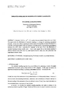
performance close to maximum. This will save optimization time and thus speed up architecture exploration. B. Simulated Annealing SA is a probabilistic non-greedy algorithm [1] that explores search space of a problem by annealing from a high to a low temperature state. The algorithm always accepts a move into a better state, but also into a worse state with a changing probability. This probability decreases along with the temperature, and thus the algorithm becomes greedier. The algorithm terminates when the final temperature is reached and sufficient number of consecutive moves have been rejected. Fig. 1 shows the pseudo-code of the SA algorithm used with the new method for parameter selection. Implementation specific issues compared to the original algorithm are explained in Section III. The Cost function evaluates execution time of a specific mapping by calling the scheduler. S0 is the initial mapping of the system, T0 is the initial temperature, and S and T are current mapping and temperature, respectively. New Temperature Cooling function, a contribution of this paper, computes a new temperature as a function of initial temperature T0 and iteration i. R is the number of consecutive rejects. M ove function moves a random task to a random PE, different than the original PE. Random function returns an uniform random value from the interval [0, 1). New Prob function, a contribution of this paper, computes a probability for accepting a move that increases the cost. Rmax is the maximum number of consecutive rejections allowed after the final temperature has been reached. III. T HE PARAMETER S ELECTION M ETHOD The parameter selection method configures the annealing schedule and acceptance probability functions. N ew T emperature Cooling function is chosen so that annealing schedule length is proportional to application and system architecture size. Moreover the initial temperature T0 and final temperature Tf must be in the relevant range to affect acceptance probabilities efficiently. The method uses i
N ew T emperature Cooling(T0 , i) = T0 ∗ q b L c , where L is the number of mapping iterations per temperature level and q is the proportion of temperature preserved after each temperature level. This paper uses q = 0.95. Determining proper L value is important to anneal more iterations for larger applications and systems. This method uses L = N (M − 1), where N is the number of tasks and M is the number of processors in the system. Also, Rmax = L. A traditionally used acceptance function is T rad P rob(∆C, T ) =
1 , 1 + exp( ∆C T )
but then probability range for accepting moves is not adjusted to a given task graphs because ∆C is not normalized. The acceptance probability function used in this method has a
S IMULATED A NNEALING(S0 , T0 ) 1 S ← S0 2 C ← C OST(S0 ) 3 Sbest ← S 4 Cbest ← C 5 R←0 6 for i ← 0 to ∞ 7 do T ← N EW T EMPERATURE C OOLING(T0 , i) 8 Snew ← M OVE(S, T ) 9 Cnew ← C OST(Snew ) 10 ∆C ← Cnew − C 11 r ← R ANDOM () 12 p ← N EW P ROB(∆C, T ) 13 if ∆C < 0 or r < p 14 then if Cnew < Cbest 15 then Sbest ← Snew 16 Cbest ← Cnew 17 S ← Snew 18 C ← Cnew 19 R←0 20 else if T ≤ Tf 21 then R ← R + 1 22 if R ≥ Rmax 23 then break 24 return Sbest Fig. 1.
Pseudo-code of the simulated annealing algorithm
normalization factor to consider only relative cost function changes. Relative cost function change adapts automatically to different cost function value ranges and graphs with different task execution times. N ew P rob(∆C, T ) =
1 , ∆C ) 1 + exp( 0.5C 0T
where C0 = Cost(S0 ), the initial cost of the optimized system. Figure 2 shows relative acceptance probabilities. The initial temperature chosen by the method is T0P =
ktmax tminsum
,
where tmax is the maximum execution time for any task on any processor, tminsum the sum of execution times for all tasks on the fastest processor in the system, and k ≥ 1 is a constant. Constant k, which should practically be less than 10, gives a temperature margin for safety. Section IV-A will show that k = 1 is sufficient in our experiment. The rationale is choosing an initial temperature where the biggest single task will have a fair transition probability of being moved from one PE to another. The transition probabilities with respect to temperature and ∆Cr = ∆C C0 can be seen in Figure 2. Section IV will show that efficient annealing happens in the temperature range predicted by the method. The chosen final temperature is TfP =
tmin , ktmaxsum
Acceptance probability of a move to worse state
0.5
TABLE I
0.45
O PTIMIZATION PARAMETERS FOR THE EXPERIMENT
0.4
Parameter L T0 Tf M N
∆Cr = 0.0001
0.35 ∆Cr = 0.0010 0.3 0.25
∆Cr = 0.0100
0.2
0.1
Meaning Iterations per temperature level Initial temperature Final temperature Number of processors Number of tasks
4
∆Cr = 0.1000
0.15
Value 1, 2, 4, . . . , 4096 1 10−4 2-8 50, 300
∆Cr = 1.0000
3.5
0.05
Fig. 2.
−3
10
−2
10 Temperature
−1
10
0
10
Probabilities for the normalized probability function: ∆Cr =
3
∆C C0
where tmin is the minimum execution time for any task on any processor and tmaxsum the sum of execution times for all tasks on the slowest processor in the system. Choosing initial and final temperature properly will save optimization iterations. On too big a temperature, the optimization is practically Monte Carlo optimization because it accepts moves to worse positions with a high probability. And thus, it will converge very slowly to optimum because the search space size is in O(M N ). Also, too low a probability reduces the annealing to greedy optimization. Greedy optimization becomes useless after a short time because it can not espace local minima. IV. R ESULTS A. Experiment The experiment uses 10 random graphs with 50 nodes and 10 random graphs with 300 nodes from the Standard Task Graph set [7] to validate that the parameter selection method chooses good acceptance probabilities (N ew P rob) and annealing schedule (T0P , TfP , and L). Random graphs are used to evaluate optimization algorithms as fairly as possible. Non-random applications may well be relevant for common applications, but they are dangerously biased for general parameter estimation. Investigating algorithm bias and classifying computational tasks based on the bias are not topics of this paper. Random graphs have the property to be neutral of the application. Optimization was run 10 times independently for each task graph. Each graph was distributed onto 2-8 PEs. Each anneal was run from a high temperature T0 = 1.0 to a low temperature Tf = 10−4 with 13 different L values. The experiment will show that [Tf , T0 ] is a wide enough temperature range for optimization and that [TfP , T0P ] is a proper subset of [Tf , T0 ] which will yield equally good results in a smaller optimization time. L values are powers of 2 to test a wide range of suitable parameters. All results were averaged for statistical reliability. The optimization parameters of the experiment are shown in Table I. The SoC platform was a message passing system where each PE had some local memory, but no shared memory. The PEs were interconnected with a single dynamically arbitrated
Average speedup
0 −4 10
2.5
L = 1−4096
2
1.5
1
2
3
4
5 Number of PEs
6
7
8
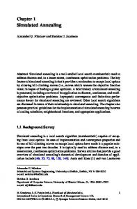
Fig. 3. Averaged speedups for 300 node graphs with M =2-8 processing elements and different L values (L = 1, 2, . . . , 4096) for each processing element set.
shared bus that limits the SoC performance because of bus contention. The optimization software was written in C language and executed on a 10 machine Gentoo Linux cluster each machine having a 2.8 GHz Intel Pentium 4 processor and 1 GiB of memory. A total of 2.03G mappings were tried . in 909 computation hours leading to average 620 mappings s B. Experimental Results Figure 3 shows averaged speedups for 300-node task graphs with respect to number of iterations per temperature level and number of PEs. Speedup is defined as ttM1 , where ti is the graph execution time on i PEs. The bars show that selecting L = N (M − 1), where N = 300 is the number of tasks and M ∈ [2, 8] gives sufficient iterations per temperature level to achieve near best speedup (over 90% in this experiment) when the reference speedup is L = 4096. The Figure also shows that higher number of PEs requires higher L value which is logically consistent with the fact that higher number of PEs means to a bigger optimization space. Figure 4 shows average speedup with respect to temperature. Average execution time proportion for a single task in a 300 1 node graph is 300 = 0.0033. With our normalized acceptance probability function this also means the interesting temperature value for annealing, T = 0.0033, falls safely within the predicted temperature range [TfP , T0P ] = [0.0004, 0.0074] computed with k = 1 from 300 node graphs. The Figure shows that optimization progress is fastest at that range. The full range [Tf , T0 ] was annealed to show convergence outside
3
3 Predicted range
L = 4096 iterations L = 256 L = 64 L = 16 L=1
2.8
2.6
2.4
Average speedup when M = 2−8
Average speedup when M=2−8
2.6
2.8
SA opt. progress
2.2 2 1.8 SA region
"Monte Carlo"
1.6
−2
−1
0
10
10
Fig. 4. Averaged speedup with respect to temperature for 300 node graphs with different L values. 3
1.6
2.6
1
10
2
10
3
10 Evaluated mappings
4
10
5
10
6
10
Fig. 6. Averaged speedup with respect to mapping evaluations for 300 node graphs with different L values.
V. C ONCLUSION
2.4 2.2 2 1.8 1.6 Predicted range 1.4 1.2 1 −4 10
1 0 10
This Figure also strenghtens the hypothesis that L = N (M − 1) = 300, . . . , 2100 is sufficient number of iterations per temperature level.
L = 4096 L = 256 L = 64 L = 16 L=1
2.8
Average speedup when M = 2−8
1.8
1.2
10 Temperature
16
2
1.2
−3
64
2.2
1.4
10
256
2.4
1.4
1 −4 10
4096
L = 4096 iterations L = 256 L = 64 L = 16 L=1
−3
10
−2
10 Temperature
−1
10
0
10
Fig. 5. Averaged speedup with respect to temperature for 50 node graphs with different L values.
the predicted range. The method also applies well for the 50 node graphs, as shown in Figure 5, where the interesting 1 = 0.02. The predicted range temperature point is at T = 50 computed for 50 node graphs with k = 1 is [0.0023, 0.033] and the Figure shows that steepest optimization progress falls within that range. Annealing the temperature range [10−2 , 1] with 300 nodes in Figure 4 is avoided by using the parameter selection method. That range is essentially Monte Carlo optimization which converges very slowly and is therefore unnecessary. The temperature scale is exponential and therefore that range consists of half the total temperature levels in the range [Tf , T0 ]. This means approximately 50% of optimization time can be saved by using the parameter selection method. The main benefit of this method is determining an efficient annealing schedule. The average speedups with respect to number of mapping evaluations with different L values is shown in Figure 6. Optimization time is a linear function of evaluated mappings.
The new parameter selection method was able to predict an efficient annealing schedule for simulated annealing to both maximize application execution performance and also minimize optimization time. Near maximum performance was achieved by selecting the temperature range and setting the number of iterations per temperature level automatically based on application and platform size. The number of temperature levels was halved by the method. Thus the method increased accuracy of architecture exploration and accelerated it. Further research is needed to investigate simulated annealing heuristics that explore new states in the mapping space. A good choice of mapping heuristics can improve solutions and accelerate convergence, and it is easily applied into the existing system. Further research should also investigate how this method applies to optimizing memory, power consumption, and other factors in a SoC. R EFERENCES [1] S. Kirkpatrick, C. D. Gelatt Jr., M. P. Vecchi, Optimization by simulated annealing, Science, Vol. 200, No. 4598, pp. 671-680, 1983. [2] Y.-K. Kwok and I. Ahmad, Static scheduling algorithms for allocating directed task graphs to multiprocessors, ACM Comput. Surv., Vol. 31, No. 4, pp. 406-471, 1999. [3] H. Orsila, T. Kangas, T. D. H¨am¨al¨ainen, Hybrid Algorithm for Mapping Static Task Graphs on Multiprocessor SoCs, International Symposium on System-on-Chip (SoC 2005), pp. 146-150, 2005. [4] T. Wild, W. Brunnbauer, J. Foag, and N. Pazos, Mapping and scheduling for architecture exploration of networking SoCs, Proc. 16th Int. Conference on VLSI Design, pp. 376-381, 2003. [5] F. Glover, E. Taillard, D. de Werra, A User’s Guide to Tabu Search, Annals of Operations Research, Vol. 21, pp. 3-28, 1993. [6] T. D. Braun, H. J. Siegel, N. Beck, A Comparison of Eleven Static Heuristics for Mapping a Class if Independent Tasks onto Heterogeneous Distributed Systems, IEEE Journal of Parallel and Distributed Computing, Vol. 61, pp. 810-837, 2001. [7] Standard task graph set, [online]: http://www.kasahara.elec.waseda.ac.jp/schedule, 2003.