Passive Mobile Robot Localization within a Fixed Beacon ... - CiteSeerX

Proc. WAFR (Seventh International Workshop on the Algorithmic Foundations of Robotics), New York, NY, July 2006

Passive Mobile Robot Localization within a Fixed Beacon Field Carrick Detweiler, John Leonard, Daniela Rus, and Seth Teller Computer Science and Artificial Intelligence Laboratory, Massachusetts Institute of Technology, {carrick,jleondard,rus,teller}@csail.mit.edu Abstract: This paper describes an intuitive geometric algorithm for the localization of mobile nodes in networks of sensors and robots using range-only or angle-only measurements. The algorithm is a minimalistic approach to localization and tracking when dead reckoning is too inaccurate to be useful. The only knowledge required about the mobile node is its maximum speed. Geometric regions are formed and grown to account for the motion of the mobile node. New measurements introduce new constraints which are propagated back in time to refine previous localization regions. The mobile robots are passive listeners while the sensor nodes actively broadcast making the algorithm scalable to many mobile nodes while maintaining the privacy of individual nodes. We prove that the localization regions found are optimal–that is, they are the smallest regions which must contain the mobile node at that time. We prove that each new measurement requires quadratic time in the number of measurements to update the system, however, we demonstrate experimentally that this can be reduced to constant time.

1 Introduction Localization is a critical issue for many field robotics applications. In open outdoor environments, differential GPS systems can provide precise positioning information. There are many applications, however, in which GPS cannot be used, such as indoor, underwater, extraterrestrial, or urban environments. For situations when GPS is unavailable, dead reckoning may provide an alternative. Dead reckoning, however, is subject to accumulated error over time and is insufficient for many tasks. Most current localization methods make use of range or angle measurements to other nodes (pre-deployed beacons or other robots) to constrain dead reckoning error growth [4, 7, 14, 15, 19, 20]. In this paper, we present a localization algorithm for mobile agents for situations in which dead reckoning capabilities are poor, or simply unavailable. This includes the important case of passively tracking a non-cooperative target. The method is also applicable to low cost underwater robots, such as

2

Carrick Detweiler, John Leonard, Daniela Rus, and Seth Teller

AMOUR [25], and other non-robotic mobile agents, such as animals [2] and people [10]. Our approach is based on a field of statically fixed nodes that communicate within a limited distance and are capable of estimating either ranges (in one case) or angles (in the other case) to neighbors. These agents are assumed to have been previously localized by a static localization algorithm (e.g. [18]). A mobile node moves through this field, passively obtaining ranges (respectively angles) to nearby fixed nodes and listens to broadcasts from the static nodes. Based on this information, and an upper bound on the speed of the mobile node, our method recovers an estimate of the path traversed. As additional measurements are obtained, this new information is propagated backwards to refine previous location estimates. We prove that our algorithm finds optimal localization regions–that is, the smallest regions that must contain the mobile node. Our algorithm allows for significant delays between measurements which makes traditional trilateration or triangulation approaches impossible. The algorithm is scalable to any number of mobile nodes as the mobile nodes are passive. The passivity of listeners also maintains the privacy of the mobile nodes. This paper is organized as follows. We first introduce the intuition behind the range-only and angle-only versions of the algorithm. We then present the general algorithm, which can be instantiated with either range or angle information, and prove that it is optimal. Finally, we discuss an implementation of the range-only and angle-only algorithms, present experimental results of the range-only algorithm, and discuss extensions to the algorithm.

2 Related Work A wide variety of strategies have been pursued for representing uncertainty in robot localization. Many approaches employ probabilistic state estimation to compute a posterior for the robot trajectory, based on assumed measurement and motion models. A variety of filtering methods have been employed for localization of mobile robots, including EKFs [7, 14, 15], Markov methods [3, 14], Monte Carlo methods [6, 7, 14] and batch techniques [4, 14, 15, 16]. Much of this recent work falls into the broad area of simultaneous localization and mapping (SLAM), in which the goal is to concurrently build a map of an unknown environment while localizing the robot. Our approach assumes that the robot operates in a static field of nodes whose positions are known a priori. We assume only a known velocity bound for the vehicle, in contrast to the more detailed motion models assumed by modern SLAM methods. Most current localization algorithms assume an accurate model of the vehicle’s uncertain motion. If a detailed probabilistic model is available, then a state estimation approach will likely produce a more accurate trajectory estimate for the robot. There are numerous real-world sit-

Passive Mobile Robot Localization within a Fixed Beacon Field

3

uations, however, that require localization algorithms that can operate with minimal proprioceptive sensing, poor motion models, and/or highly nonlinear measurement constraints. In these situations, the adoption of a bounded error representation, instead of a representation based on Gaussians or particles, is justified. In previous work, Smith et al. also explored the problem of localization of mobile nodes without dead reckoning [22]. They compare the case where the mobile node is a passive listener verses actively pinging to obtain range estimates. In the passive listening case an EKF is used. However, the inherent difficulty of (re)initializing the filter leads them to conclude a hybrid approach is necessary. The mobile node remains passive until it detects a bad state. At this point it becomes active. In our work we maintain a passive state. Additionally, our approach introduces a geometric approach to localization which can stand alone, as we demonstrate experimentally in Section 6, or be post-processed by a Kalman filter or other filtering methods. Our approach represents uncertainty using bounded regions that are computed based on worst-case assumptions of dead-reckoning and measurement errors. This can be contrasted with the conventional assumption of Gaussian errors in EKF approaches, or the representation of uncertainty with sets of particles in Markov Chain Monte Carlo state estimation [24]. Previous work adopting a bounded region representation of uncertainty includes Meizel et al. [17], Briechle and Hanebeck [1], Spletzer and Taylor [23], and Isler and Bajcsy [12]. Meizel et al. investigated the initial location estimation problem for a single robot given a prior geometric model based on noisy sonar range measurements. Briechle and Hanebeck [1] formulated a bounded uncertainty pose estimation algorithm given noisy relative angle measurements to point features. Doherty et al. [9] investigated localizations methods based only on wireless connectivity, with no range estimation. Spletzer and Taylor developed an algorithm for multi-robot localization based on a bounded uncertainty model [23]. Finally, Isler and Bajscy examine the sensor selection problem based on bounded uncertainty models [12]. The robot localization problem bears similarities with the classical problem of robot motion planning with uncertainty. In the seminal work of Erdmann bounded sets are used for forward projection of possible robot configurations. These are restricted by the control uncertainty cone [11]. In our work the step to compute the set of feasible poses for a robot moving through time is similar to Erdmann’s forward projection step. Our approach differs from all these approaches by incorporating a dynamic motion component for the robot. By assuming a worst-case model for robot motion, in terms of a maximum allowable speed, we are able to develop a bounded region localization algorithm that can handle the trajectory estimation problem given non-simultaneous measurements. This scenario is particularly important for underwater acoustic tracking applications, where significant delays between measurements are common due to the speed of sound.

4

Carrick Detweiler, John Leonard, Daniela Rus, and Seth Teller

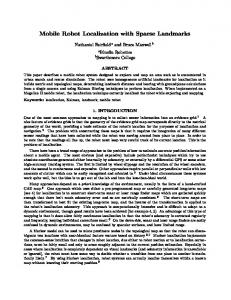
3 Algorithm Intuition This section formally describes the localization problem we solve and the intuition behind the range-only version and angle-only version of the localization algorithms. The generic algorithm is presented in section 4. 3.1 Problem Formulation We will now define a generic formulation for the localization problem. This setup can be used to evaluate range-only, angle-only, and other localization problems. We start by defining a localization region. Definition 1. A localization region at some time t is the set of points in which a node is assumed to be at time t. We will often refer to a localization region simply as a region. It is useful to formulate the localization problem in terms of regions as the problem is typically under-constrained, so exact solutions are not possible. Probabilistic regions can also be used, however, we will use a discrete formulation. In this framework the localization problem can be stated in terms of finding optimal localization regions. Definition 2. We say that a localization region is optimal with respect to a set of measurements at time t if at that time it is the smallest region that must contain the true location of the mobile node, given the measurements and the known velocity bound. A region is individually optimal if it is optimal with respect to a single measurement. For example, for a range measurement the individually optimal region is an annulus and for the angle case it is a cone. Another way to phrase optimality is if a region is optimal at some time t, then the region contains the true location of the mobile node and all points in the region are reachable by the mobile node. Suppose that from time 1 · · · t we are given regions A1 · · · At each of which is individually optimal. The times need not be uniformly distributed, however, we will assume that they are in sorted order. By definition, at time k region Ak must contain the true location of the mobile node and furthermore, if this is the only information we have about the mobile node, it is the smallest region that must contain the true location. We now want to form regions, I1 · · · It , which are optimal given all the regions A1 · · · At and an upper bound on the speed of the mobile node which we will call s. We will refer to these regions as intersection regions as they will be formed by intersecting regions. 3.2 Range-Only Localization and Tracking Figure 1 shows critical steps in the range-only localization of mobile Node m. Node m is moving through a field of localized static nodes (Nodes a, b, c) along the trajectory indicated by the dotted line.

Passive Mobile Robot Localization within a Fixed Beacon Field

(a)

(b)

(d)

5

(c)

(e)

(f)

Fig. 1. Example of the range-only localization algorithm.

At time t Node m passively obtains a range to Node a. This allows Node m to localize itself to the circle indicated in Figure 1(a). At time t + 1 Node m has moved along the trajectory as shown in Figure 1(b). It expands its localization estimation to the annulus in Figure 1(b). Node m then enters the communication range of Node b and obtains a ranging to Node b (see Figure 1(c)). Next, Node m intersects the circle and annulus to obtain a localization region for time t + 1 as indicated by the bold red arcs in Figure 1(d). The range taken at time t + 1 can be used to improve the localization at time t as shown in Figure 1(e). The arcs from time t + 1 are expanded to account for all locations the mobile node could have come from. This is then intersected with the range taken at time t to obtain the refined location region illustrated by the bold blue arcs. Figure 1(f) shows the final result. Note that for times t and t + 1 there are two possible location regions. This is because two range measurements do not provide sufficient information to fully constrain the system. Range measurements from other nodes will quickly eliminate this. 3.3 Angle-Only Localization and Tracking Consider Figure 2. Each snapshot shows three static nodes that have selflocalized (Nodes a, b, c). Node m is a mobile node moving through the field of static nodes along the trajectory indicated by the dotted line. Each snapshot shows a critical point in the angle-only location and trajectory estimation for Node m.

6

Carrick Detweiler, John Leonard, Daniela Rus, and Seth Teller

(a)

(d)

(b)

(e)

(c)

(f)

Fig. 2. Example of the angle-only localization algorithm.

At time t Node m enters the communication range of Node a and passively computes the angle to Node a. This allows Node m to estimate its position to be along the line shown in Figure 2(a). At time t + 1 Node m has moved as shown in Figure 2(b). Based on its maximum possible speed, Node m expands its location estimate to that shown in Figure 2(b). Node m now obtains an angle measurement to Node b as shown in Figure 2(c). Based on the intersection of the region and the angle measurement Node m can constrain its location at time t + 1 to be the bold red line indicated in Figure 2(d). The angle measurement at time t + 1 can be used to further refine the position estimate of the mobile node at time t as shown in Figure 2(e). The line that Node m was localized to at time t + 1 is expanded to represent all possible locations Node m could have come from. This is region is then intersected with the original angle measurement from Node a to obtain the bold blue line which is the refined localization estimate of Node m at time t. Figure 2(f) shows the two resulting location regions. New angle measurements will further refine these regions.

4 The Localization Algorithm 4.1 Generic Algorithm The localization algorithm follows the same idea as in Section 3. Each new region computed will be intersected with the grown version of the previous

Passive Mobile Robot Localization within a Fixed Beacon Field

7

region and the information gained from the new region will be propagated backwards. Algorithm 1 shows the details. Algorithm 1 Localization Algorithm 1: procedure Localize(A1 · · · At ) 2: s ← max speed 3: I1 = A1 4: for k = 2 to t do 5: 4t ← k − (k − 1) 6: Ik =Grow(Ik−1 , s4t) ∩ Ak 7: for j = k − 1 to 1 do 8: 4t ← j − (j − 1) 9: Ij =Grow(Ij+1 , s4t) ∩ Aj 10: end for 11: end for 12: end procedure

. Initialize the first intersection region

. Create the new intersection region . Propagate measurements back

Algorithm 1 can be run online by omitting the outer loop (lines 4-6 and 11) and executing the inner loop whenever a new region/measurement is obtained. The first step in Algorithm 1 (line 3), is to initialize the first intersection region to be the first region. Then we iterate through each successive region. The new region is intersected with the previous intersection region grown to account for any motion (line 6). Finally, the information gained from the new region is propagated back by successively intersecting each optimal region grown backwards with the previous region, as shown in line 9. 4.2 Algorithm Details Two key operations in the algorithm which we will now examine in detail are Grow and Intersect. Grow accounts for the motion of the mobile node over time. Intersect produces a region that contains only those points found in both localization regions being intersected.

Fig. 3. Growing a region by s. Acute angles, when grown, turn into circles as illustrated. Obtuse angles, on the other hand, are eventually consumed by the growth of the surroundings.

8

Carrick Detweiler, John Leonard, Daniela Rus, and Seth Teller

Figure 3 illustrates how a region grows. Let the region bounded by the black lines contain the mobile node at time t. To determine the smallest possible region that must contain the mobile node at time t+1 we Grow the region by s, where s is the maximum speed of the mobile node. The Grow operation is the Minkowski sum [8] (frequently used in motion planning) of the region and a circle with diameter s. Notice that obtuse corners become circle arcs when grown, while everything else “expands.” If a region is convex, it will remain convex. Let the complexity of a region be the number of simple geometric features (lines and circles) needed to describe it. Growing convex regions will never increase the complexity of a region by more than a constant factor. This is true as everything just expands except for obtuse angles which are turned into circles and there are never more than a linear number of obtuse angles. Thus, growing can be done in time proportional to the complexity of the region. A simple algorithm for Intersect is to check each feature of one region for intersection with all features of the other region. This can be done in time proportional to the product of the complexities of the two regions. While better algorithms exist for this, for our purposes this is sufficient as we will always ensure that one of the regions we are intersecting has constant complexity as shown in Sections 5.2 and 5.3. Additionally, if both regions are convex, the intersection will also be convex. 4.3 Correctness and Optimality We now prove the correctness and optimality of Algorithm 1. We will show that the algorithm finds the location region of the node, and that this computed location region is the smallest region that can be determined using only maximum speed. We assume that the individual regions given as input are optimal, which is trivially true for both the range and angle-only cases. Theorem 1. Given the maximum speed of a mobile node and t individually optimal regions, A1 · · · At , Algorithm 1 will produce optimal intersection regions I1 · · · It . Without loss of generality assume that A1 · · · At are in time order. We will prove this theorem inductively on the number of range measurements for the online version of the localization algorithm. The base case is when there is only a single range measurement. Line 3 implies I1 = A1 and we already know A1 is optimal. Now inductively assume that intersection regions I1 · · · It−1 are optimal. We must now show that when we add region At , It is optimal and the update of I1 · · · It−1 maintains optimality given this new information. Call these updated 0 intersection regions I10 · · · It−1 . First we will show that the new intersection region, It0 , is optimal. Line 6 of the localization algorithm is

Passive Mobile Robot Localization within a Fixed Beacon Field

It0 = Grow(It−1 , s4t) ∩ At .

9

(1)

The region Grow(It−1 ) contains all possible locations of the mobile node at time t ignoring the measurement At . The intersection region It0 must contain all possible locations of the mobile node as it is the intersection of two regions that constrain the location of the mobile node. If this were not the case, then there would be some point p which was not in the intersection. This would imply that p was neither in It−1 nor At , a contradiction as this would mean p was not reachable. Additionally, all points in It0 are reachable as it is the intersection of a reachable region with another region. Therefore, It0 is optimal. Finally we will show that the propagation backwards, line 9, produces optimal regions. The propagation is given by 0 Ij0 = Grow(Ij+1 , s4t) ∩ Aj

(2)

for all 1 ≤ j ≤ t − 1. The algorithm starts with j = t − 1. We just showed that It0 is optimal, so using the same argument as above It−1 is optimal. Applying this recursively, all It−2 · · · I1 are optimal. Q.E.D.

5 Complexity 5.1 General Complexity Algorithm 1 has both an inner and outer loop over all regions which suggests an O(n2 ) runtime, where n is the number of input regions. However, Grow and Intersect also take O(n) time as proven later by Theorem 2 and 3 for the range and angle only cases. Thus, overall, we have an algorithm which runs in O(n3 ) time. We show, however, that we expect the cost of Grow and Intersect will be O(1), which suggests O(n2 ) runtime overall. The runtime can be further improved by noting that the correlation of the current measurement with the past will typically decrease rapidly as time increases. This implies that information need only be propagated back a fixed number of steps, eliminating the inner loop of Algorithm 1. Thus, we can reduce the complexity of the algorithm to O(n). 5.2 Range-Only Complexity The range-only instantiation of Algorithm 1 is obtained by taking range measurements to the nodes in the sensor fields. Let A1 · · · An be the circular regions formed by n range measurements. A1 · · · An are individually optimal and as such can be used as input to Algorithm 1. We now prove the complexity of localization regions is worst case O(n). Experimentally we find they are actually O(1) leading to an O(n2 ) runtime. Theorem 2. The complexity of the regions formed by the range-only version of the localization algorithm is O(n), where n is the number of regions.

10

Carrick Detweiler, John Leonard, Daniela Rus, and Seth Teller

The algorithm intersects a grown intersection region with a regular region. This will be the intersection of some grown segments of an annulus with a circle (as shown in the Figure 4). Let regions that contain multiple disjoint sub-regions be called compound regions. Since one of the regions is always composed of simple arcs, the result of an intersection will be a collection of circle segments. We will show that each intersection can at most increase the number of circle segments by two, implying linear complexity in the worst case.

Fig. 4. An example compound intersection region (in blue) and some new range measurement in red. With each iteration it is possible to increase the number of regions in the compound intersection region by at most two.

Consider Figure 4. At most the circular region can cross the inner circle of the annulus that contains the compound region twice. Similarly, the circle can cross the outer circle of the annulus at most twice. The only way the number of sub-regions formed can increase is if the circle enters a sub-region, exits that sub-region, and then reenters it as illustrated in the figure. If any of the entering or exiting involves crossing the inner or outer circles of the annulus, then it must cross at least twice. This means that at most two regions could be split using this method, implying a maximum increase in the number of regions of at most two. If the circle does not cut the interior or exterior of the annulus within a sub-region then it must enter and exit though the ends of the sub-region. But notice that the ends of the sub-regions are grown such that they are circular, so the circle being intersected can only cross each end twice. Furthermore, the only way to split the subregion is to cross both ends. To do this the annulus must be entered and exited on each end, implying all of the crosses of the annulus have been used up. Therefore, the number of regions can only be increased by two with each intersection proving Theorem 2. In practice it is unlikely that the regions will have linear complexity. As seen in Figure 4 the circle which is intersecting the compound region must be very precisely aligned to increase the number of regions (note that the bottom

Passive Mobile Robot Localization within a Fixed Beacon Field

11

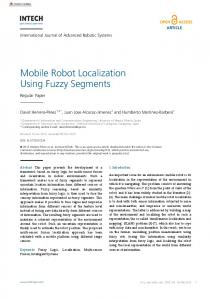
circle does not increase the number of regions). In the experiments described in Section 6 we found some regions divided in two or three (e.g. when there are only two range measurements, recall Figure 1). However, there were none with more than three sub-regions. Thus, in practice the complexity of the regions is constant leading to O(n2 ) runtime. 5.3 Angle-Only Region Complexity Algorithm 1 is instantiated in the angle-only case by taking angle measurements θ1 · · · θt with corresponding bounded errors e1 · · · et to the field of sensors. These form the individually optimal regions A1 · · · At used as input to Algorithm 1. These regions appear as triangular wedges as shown in Figure 5(a). We now show the complexity of the localization regions is at worst O(n) letting us conclude an O(n3 ) algorithm (in practice, the complexity is O(1) implying a runtime of O(n2 ) see below). Theorem 3. The complexity of the regions formed by the angle-only version of the localization algorithm is O(n), where n is the number of regions.

22

20

Region Complexity

18

16

14

12

10

8

6

(a)

0

50

100 150 Number of Grows and Intersections

200

250

(b)

Fig. 5. (a)An example of the intersecting an angle measurement region with another region. Notice that the bottom line increases the complexity of the region by one, while the top line decreases the complexity of the region by two. (b)Growth in complexity of a localization region as a function of the number of Grow and Intersect operations.

Examining the Algorithm 1, each of the intersection regions I1 · · · In are formed by intersecting a region with a grown intersection region n times. We know growing a region never increases the complexity of the region by more than a constant factor. We will now show that intersecting a region with a

12

Carrick Detweiler, John Leonard, Daniela Rus, and Seth Teller

grown region will never cause the complexity of the new region to increase by more than a constant factor. Each of these regions is convex as we start with convex regions and Grow and Intersect preserve convexity. Assume we are intersecting Grow(Ik ) with Ak−1 . Note that Ak−1 is composed of two lines. As Grow(Ik ) is convex, each line of Ak−1 can only enter and exit Grow(Ik ) once. Most of the time this will actually decrease the complexity as it will “cut” away part of the region. The only time that it will increase the complexity is when the line enters a simple feature and exits on the adjacent one as shown in Figure 5(a). This increases the complexity by one. Thus, with the two lines from the region Ak−1 the complexity is increased by at most two. In practice the complexity of the regions is not linear, rather it is constant. When a region is intersected with another region there is a high probability that some of the complex parts of the region will actually be removed, simplifying the region. Figure 5(b) illustrates the results of a simulation where the complexity of a region was tracked over time. In the simulation a single region was repeatedly grown and then intersected with a region formed by an angle measurement from a randomly chosen node from a field of 30 static nodes. Figure 5(b) shows that increasing the number of intersections does not increase the complexity of the region. The average complexity of the region was 12.0. Thus, the complexity of the regions is constant so the angle-only localization algorithm runs in O(n2 ).

6 Experimental Results We implemented the range-only version of Algorithm 1 and tested it on a dataset created by Moore et al. [18]. Range measurements were obtained from a static network of six MIT Crickets [21] to one mounted on a mobile robot. The robot moved within a 2.0 by 1.5 meter space. Ground truth was collected by a video capture system with sub-centimeter accuracy [18]. Figure 6(a) shows the static nodes (green), the arcs recovered by the localization algorithm (orange), and a path generated by connecting the mid-points of the arcs (green). Figure 6(b) shows the same recovered trajectory (green) along with ground truth data (red). Inset in Figure 6(b) is an enlarged view showing a location where an error occurred due to a lack of measurements while the robot was making a turn. The mean absolute error from the ground truth was 7.0cm with a maximum of 15.6cm. This was computed by taking the absolute error from the ground truth data at each point in the recovered path. This compares well with the 5cm of measurement error inherent to the Crickets [18]. Figure 7 shows the absolute error as a function of time. The algorithm handles the error intrinsic to the sensors well. One reason for this is the robot did not always travel at its maximum speed in a straight line. This meant the regions were larger than if the robot were traveling at its

Passive Mobile Robot Localization within a Fixed Beacon Field

(a)

13

(b)

Fig. 6. (a)The arcs found by the range-only implementation of Algorithm 1 and the path reconstructed from these. Orange arcs represent the raw regions, while the green line connects the midpoints of these arcs. (b)Ground truth (red) and recovered path (green). Inset is an enlarged portion illustrating error caused by a lack of measurements during a turn of the robot.

maximum speed in a straight line, making up for measurement error. In most applications this will be the case, however, to be conservative the maximum speed could be increased slightly to account for error in the sensors. Most sensors also have occasional large non-Gaussian errors. To account for these, measurements which have no intersection with the current localization region are rejected as outliers. This implementation only propagates information back to 5-8 localization regions. We did not find it sensitive to the exact number. We also never encountered a region with a complexity higher than three. These two facts gives an overall runtime of O(n), or O(1) for each new range measurement.

7 Discussion The propagation of the information gained from new measurements back to previous measurements can take a significant amount of time. In the experiments presented in Section 6 we found that we only had to propagate the information back through a small, fixed, period of time. This led to a significant reduction in the runtime. There are, however, cases where further propagation may be needed. For instance, the localization of a mobile node

14

Carrick Detweiler, John Leonard, Daniela Rus, and Seth Teller 16

14

Absolute Error (cm)

12

10

8

6

4

2

0

0

200

400

600

800

1000

1200

1400

Time

Fig. 7. Absolute error in the recovered position estimates in centimeters as a function of time.

traveling in a straight line at maximum speed could be improved by propagating the measurements back far. An adaptive system that decides at runtime how far to propagate information back may improve localization results while maintaining the constant time update. Additional knowledge about the motion characteristics of the mobile node can also be added to the system to further refine localization. Maximum acceleration is likely to be known in most physical systems. With a bound on acceleration the regions need only be grown in the current estimate of the direction of travel and directions that could be achieved by the bounded acceleration. In many systems this would significantly reduce the size of the localization regions. With real sensors there are some pathological cases which will cause the algorithm to fail. If the maximum speed has not been increased sufficiently to account for sensor errors then a number of consecutive erroneous measurements could produce a region which does not contain the true location of the mobile node. This situation can be detected as subsequent measurements will have no intersection with the current localization region. At this point the algorithm could be restarted or the previous regions could be modified to allow for a larger error. Our algorithm can be used with a variety of different sensors. Many are passive in nature which allows for the scaling of our algorithm to any number of mobile nodes. On land we have used MIT Crickets [21] to obtain range measurements. Range measurements are obtained passively by taking the difference in time of flight of a radio and ultrasonic pulse. Angle measurements can be obtained passively using an omnidirectional camera [4]. Underwater,

Passive Mobile Robot Localization within a Fixed Beacon Field

15

acoustic ranging can be done passively using synchronized clocks [5]. Angle measurements can be obtained by listening to sounds using an acoustic array [13]. The accuracy of the produced localization regions depends on a number of factors in addition to the properties of the sensors. One of the most important is the time between measurements. The more frequent the measurements the more precise the localization regions will be. Additionally, the selection of the static nodes to be used in measurements is important. For instance, taking consecutive measurements to nodes that are close together will yield poor results. Thus, a selection algorithm, such as that presented by Isler et al. [12], will improve results by choosing the best nodes for measurements. We have implemented this algorithm on our underwater robot AMOUR and underwater sensor network [25], and plan to collect data at the Gump research station in Moorea in June 2006. This system and many other underwater systems have poor dead-reckoning. We expect to enhance the localization and tracking of our robot using the algorithm presented in this paper.

References 1. K. Briechle and U. D. Hanebeck. Localization of a mobile robot using relative bearing measurements. Robotics and Automation, IEEE Transactions on, 20(1):36–44, February 2004. 2. Z. Butler, P. Corke, R. Peterson, and D. Rus. From animals to robots: virtual fences for controlling cattle. In International Symposium on Experimental Robotics, pages 4429–4436, New Orleans, 2004. 3. M. Castelnovi, A. Sgorbissa, and R. Zaccaria. Markov-localization through color features comparison. In Proceedings of the 2004 IEEE International Symposium on Intelligent Control, pages 437– 442, 2004. 4. M. Deans and M. Hebert. Experimental comparison of techniques for localization and mapping using a bearings only sensor. In Proc. of the ISER ’00 Seventh International Symposium on Experimental Robotics, pages 395–404. SpringerVerlag, December 2000. 5. M. Deffenbaugh, J. G. Bellingham, and H. Schmidt. The relationship between spherical and hyperbolic positioning. In OCEANS ’96. MTS/IEEE. ’Prospects for the 21st Century’. Conference Proceedings, volume 2, pages 590–595, 1996. 6. F. Dellaert, D. Fox, W. Burgard, and S. Thrun. Monte carlo localization for mobile robots. In IEEE International Conference on Robotics and Automation (ICRA99), volume 2, pages 1322–1328, May 1999. 7. J. Djugash, S. Singh, and P. I. Corke. Further results with localization and mapping using range from radio. In International Conference on Field and Service Robotics, July 2005. 8. D. P. Dobkin, J. Hershberger, D. G. Kirkpatrick, and S. Suri. Computing the intersection-depth of polyhedra. Algorithmica, 9(6):518–533, 1993. 9. L. Doherty, K. S. J. Pister, and L. E. Ghaoui. Convex optimization methods for sensor node position estimation. In INFOCOM, pages 1655–1663, 2001. 10. N. Eagle and A. Pentland. Reality mining: Sensing complex social systems. Personal and Ubiquitous Computing, pages 1–14, September 2005.

16

Carrick Detweiler, John Leonard, Daniela Rus, and Seth Teller

11. M. Erdmann. Using backprojections for fine motion planning with uncertainty. IJRR, 5(1):19–45, 1986. 12. V. Isler and R. Bajcsy. The sensor selection problem for bounded uncertainty sensing models. In Information Processing in Sensor Networks, 2005. IPSN 2005. Fourth International Symposium on, pages 151–158, april 2005. 13. D. Johnson and D. Dudgeon. Array Signal Processing. Prentice Hall, 1993. 14. G. A. Kantor and S. Singh. Preliminary results in range-only localization and mapping. In Proceedings of the IEEE Conference on Robotics and Automation (ICRA ’02), volume 2, pages 1818–1823, May 2002. 15. D. Kurth. Range-only robot localization and SLAM with radio. Master’s thesis, Robotics Institute Carnegie Mellon University, Pittsburgh PA, May 2004. 16. P. F. McLauchlan. A batch/recursive algorithm for 3d scene reconstruction. In Proceedings of Computer Vision and Pattern Recognition, volume 2, pages 738–743, 2000. 17. D. Meizel, O. Leveque, L. Jaulin, and E. Walter. Initial localization by set inversion. IEEE Transactions on Robotics and Automation, 18(3):966–971, December 2002. 18. D. Moore, J. Leonard, D. Rus, and S. Teller. Robust distributed network localization with noisy range measurements. In Proc. 2nd ACM SenSys, pages 50–61, Baltimore, MD, November 2004. 19. E. Olson, J. Leonard, and S. Teller. Robust range-only beacon localization. In Proceedings of Autonomous Underwater Vehicles, pages 66–75, 2004. 20. E. Olson, M. Walter, J. Leonard, and S. Teller. Single cluster graph partitioning for robotics applications. In Robotics Science and Systems, pages 265–272, 2005. 21. N. B. Priyantha, A. Chakraborty, and H. Balakrishnan. The cricket locationsupport system. In MobiCom ’00: Proceedings of the 6th annual international conference on Mobile computing and networking, pages 32–43, New York, NY, USA, 2000. ACM Press. 22. A. Smith, H. Balakrishnan, M. Goraczko, and N. Priyantha. Tracking moving devices with the cricket location system. In MobiSys ’04: Proceedings of the 2nd international conference on Mobile systems applications and services, pages 190–202, New York NY USA, 2004. ACM Press. 23. J. R. Spletzer and C. J. Taylor. A bounded uncertainty approach to multi-robot localization. In IEEE/RSJ International Conference on Intelligent Robots and Systems (IROS 2003), volume 2, pages 1258–1265, 2003. 24. S. Thrun, W. Burgard, and D. Fox. Probabilistic Robotics. MIT Press, 2005. 25. I. Vasilescu, K. Kotay, D. Rus, M. Dunbabin, and P. Corke. Data collection, storage, and retrieval with an underwater sensor network. In SenSys ’05: Proceedings of the 3rd international conference on Embedded networked sensor systems, pages 154–165, New York, NY, USA, 2005. ACM Press.