D-01062 Dresden, Germany http://www.iai.inf.tu-dresden.de/en/tis/index.html. Passive Monitoring of Control Loops in Building. Automation. Technical Report.
Chair of Technical Information Systems, Dresden University of Technology, Germany Chair of Technical Information Systems Department of Computer Science Dresden University of Technology D-01062 Dresden, Germany http://www.iai.inf.tu-dresden.de/en/tis/index.html
Passive Monitoring of Control Loops in Building Automation
Technical Report by Volodymyr Vasyutynskyy
Based on: Vasyutynskyy, V.; Plönnigs, J.; Kabitzsch, K.: Passive Monitoring of Control Loops in Building Automation. Proc. FeT2005 6th IFAC International Conference on Fieldbus Systems and their Applications, Puebla, Mexico, November 2005, pp. 263 – 269.
Technical Report, 2005
PASSIVE MONITORING OF CONTROL LOOPS IN BUILDING AUTOMATION
Volodymyr Vasyutynskyy, Joern Ploennigs, Klaus Kabitzsch Faculty of Computer Science Dresden University of Technology, D-01062 Dresden, Germany Fax: ++49 351 463 38460 E-mail: {vv3, jp14, kk10}@inf.tu-dresden.de
Abstract: The monitoring of control loop performance in building automation is important for decreasing the maintenance costs. Passive monitoring with network analyzers is inexpensive and does not influence the network load. However, control signals that are not transmitted over the network are unobservable. This paper purposes an approach to the reconstruction of missing control signals and the computation of control loop performance parameters. The analysis algorithms are adapted to the non-uniform sampling that is widely spread in building automation. Further, criteria of loop performance and network traffic for passive monitoring are introduced. Copyright © 2005 IFAC Keywords: control loops, performance monitoring, network analyzers, signal reconstruction
1. INTRODUCTION Building automation systems consist of up to several thousand heterogeneous, intelligent nodes connected by networks. They control not only heating, ventilation and air conditioning (HVAC) but also lighting, fire protection and access control. Precise models of the plants are usually unknown during the design of a building and cannot be used for finetuning of the control parameters. Instead of that, the developers use default values they know from experience as universal. This may lead to poor control loop performance, with the following disadvantages (Salsbury and Diamond, 2001): • User discomfort: deviations from setpoint, noticeable oscillations, long reaction times. • Higher energy consumption due to poor setpoint tracing. • Increased wear of control elements because of more control actions, damaged control elements in consequence of wrong control actions. All this results in increasing the maintenance costs. The effect is rather small for a single control loop, but the large number of controls in a building could lead to significant economies by their optimization. The first step in control loop optimization is the monitoring and analysis of control loop performance (CLP) (Dexter and Pakanen, 2001), which aims to detect the badly tuned loops. In this step the plant models are usually not available. CLP-monitoring is
followed by the plant model identification for the detected loops, based on the monitoring information. Finally, the controller can be retuned or replaced with another type. CLP-monitoring can be realized either with distributed or with centralized monitoring. The distributed approach requires the implementation of monitoring functions directly in the different automation nodes, which allows effective data preprocessing and fast, autonomous reaction. However, the distributed approach is limited in building automation to the simple diagnostic functions provided by the device manufacturers, since devices are usually not open for reprogramming. This limits the possibilities of a system wide optimization. The centralized approach relies on one powerful monitor to observe a whole network segment. The monitor can either collect information by polling messages actively or listen to the network traffic passively. Active monitoring increases the network load and, therefore, may provoke instabilities (Soucek and Sauter, 2004), but it is able to request information not intended by the developer to be transmitted over the network. Passive monitoring does not load the network additionally and will not interfere with the network load, and, consequently, with message transmission time and process stability. Therefore, it is predestined for loop observation.
Two effects have to be considered concerning the passive monitoring. At first, some signals cannot be observed directly, because only messages transmitted over the network can be acquired. Secondly, the transmitted messages are influenced by the network itself, i.e. they are delayed or can even get lost. As a consequence, control signals are unobservable or distorted. Moreover, non-uniform sampling is widely spread in building automation, either intended by the developer to reduce network load or caused by message delay jitter. However, usual CLP-methods presume the uniform sampling, see (Qin, 1998) and need to be adapted. These issues are considered in the proposed CLPanalysis on the basis of passive monitoring. Common control loop performance and network traffic criteria are introduced in Section 2 and opposed to the special conditions of monitoring in building automation. The reconstruction of unobservable signals is demonstrated in Section 3. In Section 4 important CLP criteria are adapted to the introduced special conditions. Further, the quality of control in networked loops is influenced by the network traffic (Lian, 2001). To estimate the coherences between these two issues, it is necessary to know the traffic parameters. The possibilities of passive monitoring in this task are investigated in Section 5.
2. MONITORING OF CONTROL LOOPS IN BUILDING AUTOMATION 2.1. Observed parameters The main objectives of the monitoring are to identify the unacceptably tuned control loops. Afterwards the measurements are gathered needed for identification of the control loop models, which is necessary for later tuning. The first objective is achieved by control loop performance analysis. Salsbury (1999) proposed a quite simple method for building automation that exploits the integral absolute error (IAE) between the plant response and the setpoint. Also the CLP-parameters used in industrial applications can be adapted to building automation systems. In general, the control loop performance parameters are divided in deterministic and stochastic ones (Qin, 1998): • Deterministic parameters depict the control loop behavior by changes of the setpoint. Those are the times characterizing the step response (rise time tr, settling time ts, time delay td) and stability parameters (overshoot, excessive oscillations in loops). • Stochastic parameters characterize the variance of the control loops in steady state (Harris, et al, 1999) and represent the stability of setpoint tracking. For networked control systems, they also include the message transmission rates and number of control actions. Some of these parameters are depicted in Figure 1. They are assessed to identify the badly tuned control loops (e.g. if they exceed required limit) and the plant models (e.g. on the basis of the rise time tr and
settling time ts as demonstrated in (Swanda and Seborg, 1999; O’Dwyer, 1999)). y(t)
Overshoot
Integral error Variance in steady state
tsettling
t
rise
t
Fig. 1. Some control loop performance parameters. 2.2. Networked control loop simulation For purpose of testing of proposed methods the simulator of networked control loops was developed. It implements the p-persistent CSMA/CD LonTalk protocol (LonTalk, 1994). The plants are presented in the simulator as a linear time-invariant system in state space with x(k +1) = A x(k) + B u(k), (1) y(k) = C x(k) + D u(k) + ξ (k). A, B, C, D are constant matrixes using parameters from the lab setup of a room automation system described in (Dementjev and Kabitzsch, 2004) and ξ(k) is a white noise. Such a simple and static plant behavior is not typical for building automation. Nevertheless, many processes change slowly and the complex plant models can be linearized in limited time intervals. Further, the control loops are controlled by PID controllers, which are widespread in building automation. It is assumed that the PID controller parameters are known (e.g. from the design databases (Ploennigs, et al, 2004)). The parameters of the plants and controllers have been varied during simulations experiments to get the different cases of loop behavior, e.g. slow, quick, oscillating or noised loops. 2.3. Passive monitoring of networked loops The passive monitoring is carried out by network analyzers, also called protocol analyzers or sniffers. They are connected to the fieldbus as shown in Figure 2 and observe online all messages passing by as an event stream. The obtained events can be interpreted in a time series of signal values according to rules formulated with help of monitoring data model purposed in (Vasyutynskyy and Kabitzsch, 2004). This enables to combine simple system events, time intervals and hierarchical sets of events (complex events) in one structure. The rules can be automatically created from the design databases (Ploennigs, et al, 2005). The observation can be provided either constantly with stationary analyzers, e.g. in combination with other maintenance services (Dementjev and Kabitzsch, 2004)); or at regular intervals, e.g. during maintenance checks.
The different steps of loop optimization imply multiple levels of complexity of the monitoring functions. In the simplest level of CLP-monitoring it should be distinguished between well-performing and badly tuned control loops. The control loops are only observed for performance problems, without precise knowing of plant models. Only for detected non-optimal controls the sophisticated and resourceconsuming analysis functions try to identify the plant models for tuning. The different monitoring levels allow observing and tuning of all control loops connected to one channel simultaneously. This paper focuses only the first level to facilitate a comprehensive description. Sensor
Actuator
S
A
Plant
C Controller
u(k)
I
M
Input device
Monitor
Fig. 2. Nodes and variables of a networked control loop. The control variables needed for CLP-monitoring can be observed without problems by network analyzers as long as their functionality is completely separated as depicted in Figure 2. But multiple functions are usually combined in one device and their control signals are unobservable. Further, the control signals may be sampled non-uniformly or distorted by communication delays. Both obstacles of passive monitoring of control loops are explained in the next two sections. 2.4. Unobservable signals In general, a control loop consists of four basic elements: a sensor (S), a controller (C), an actuator (A) and an input unit (I), where user can enter the desired setpoint. The transmitted variables are the plant input x, the plant output y and the setpoint (SP) u. Depending on the implementation several functions may be integrated in a single device, e.g. when the input unit is combined with the controller. In this case the setpoint is not transmitted over the network and is unobservable for the network analyzer. Table 1 lists the most common combinations of devices along with the observable signals.
No. 1 2 3 4 5 6
The combination of functions in one device reduces hardware costs and accelerates the communication, as the communication delays between both nodes drop out. However, it reduces the observability of control loops. In the cases 1 and 2 the setpoint signal is still known and allows applying the CLP algorithms immediately. But, for the cases 3 and 4 the setpoint signal needs to be reconstructed before the analysis algorithms can be applied. The Section 3 will develop such a reconstruction algorithm. 2.5. Node communication and signal sampling
x(k)
y(k)
introduced algorithm. The notation “C-A” means that the controller and actuator are implemented in one node.
Table 1 Node configurations Node Observable u known? configuration S, C, A, I u, x, y known S, C-A, I u, y known S, C-I, A x, y recoverable S, C-A-I y recoverable S-C-I, A x partly recoverable S-C-I-A unknown
The last column indicates whether the setpoint signal is observable or can be reconstructed with the later
Although the most processes in building automation are rather slow, high network utilization may cause serious message delays, jitters or losses, due to a large number of communicating devices. This leads to such effects like performance degradation or instability of the control loops (Lian, 2001; Koller, et al, 2003). These problems aggravate with the increasing popularity of wireless sensor networks and power line transmission, because of their smaller bandwidths and higher error rates. This influences also the CLP analysis, since the signals are in general non-uniformly sampled, that may be caused either by communication delay jitter or non-periodic sampling. In the first case, the time stamp of message record at the monitor is different from the sending time of the device, which is again different from the event time in the process. The times are shifted and jittered by all delay times during processing and transmission. As a consequence, the arrival time of messages is stochastically jittered. Even though a constant time shift can be omitted in the signal reconstruction, the jitter cannot and needs to be considered in the algorithm. Non-periodic sampling is intended to prevent the network problems by reducing the number of the transmitted messages to the minimum necessary for required control quality. The non-periodic send-ondelta, also called deadband, sampling (Otanez, et al, 2002) is broadly used in building automation. Using it, a message is transmitted only if the measured signal has changed more than a significant value ∆ since the last transmitted value, i.e. yactual − ysent > ∆ (2) Though other types of non-uniform sampling have been proposed (Yook, et al, 2000; Rehbinder and Sanfridson, 2004), the send-on-delta sampling is the most widespread. Actually, it is accepted in LONWorks standard (LON, 1994). Figure 3 compares the uniform and send-on-delta sampling for a step change of the setpoint.
∆
tmax
Send condition : t-tsent>T
Tsampling
a)
Send condition : x-xsent>∆
b)
t
Fig. 3. Step response of the control loops with uniform (a) and send-on-delta (b) sampling with the same IAE. The send-on-delta sampling results in a message silence in periods without process changes. To avoid uncertainty in this case, the parameter max-send-time tmax defines the maximum time between two messages. The allowed minimum time between subsequent messages can be limited by the min-sendtime tmin. Send-on-delta sampling is able to reduce the network load, but it also may cause instabilities in case of an error-prone connection because of the lack of the correcting messages. Further, incorrectly adjusted parameters ∆, tmax or tmin can cause aliasing and quantization oscillations near the setpoint, which not only impact the control loop performance but also increase the network load. To conclude, control signals in a networked loop are distorted by non-uniform sampling, stochastic message delay jitter and sensor noise. This requires an appropriate adjustment of the CLP-algorithms.
3. DETECTION OF SETPOINT CHANGES 3.1. Detection of setpoint change The knowledge of the setpoint signal is essential for the CLP analysis. A missing setpoint signal can be reconstructed from the process output in steady state for the cases 3 and 4 in Table 1 with the following assumptions. (A1) The setpoint needs to be changed in a step. (A2) The changes have to be infrequent with an event period significant larger than the reaction time of the control cycle. (A3) The jitter of the monitoring is negligible in comparison to the settling time. Then, the process variable mean value µ in steady state corresponds to the setpoint value u. This is quite simple, but it is necessary to identify the steady state after a step, as well as the time moment of the step change. This is possible with the algorithm introduced in subsection 3.3, but first the sampled signal needs to be reconstructed. 3.2. Signal interpolation The reconstruction of the original signal from the observed non-uniform and jittered samples is performed by interpolation. This is reasonable, as complex reconstruction algorithms require plant models, which are unknown in this step. The Shannon reconstruction presumes periodical
samples. Therefore, four simple interpolation algorithms were compared: • Hold-on of zero order (ZOH), where the value of signal is hold until the next sample comes; • Linear interpolation (first-order hold-on), where two samples are connected with a direct line; • Spline interpolation with different spline types, particularly B-splines and NURBS, and • Polynom interpolation of different grades. The methods of interpolation were compared on a set of simulated signals obtained from control loops with varied parameters like plant model parameters, PIDsettings and noise variance. The methods were compared according to two parameters. The first one is the absolute interpolation error, defined as sum of the absolute differences between real and interpolated signal. The second parameter is the accuracy of the process time estimation, defined as difference between the real process times and times defined with the help of interpolation. The results of the comparison are listed in Table 2. Table 2 Comparison of interpolation methods Method Absolute Accuracy of Computainterpolation process times tional error efforts stand-on 0.17-0.34 0.2-0.3 low linear 0.14-0.29 0.1-0.2 low spline 0.27-1.5 0.1-0.2 medium polynomial 0.29-1.45 0.1-0.2 high Hold-on interpolation is the simplest one but results in a large interpolation error and low accuracy of the estimated process times. The spline and polynomial interpolations are too sensitive to the grade of interpolation function, signal continuity and noise variance and require significant computational efforts. The linear interpolation is the most applicable one as it combines simplicity with the small interpolation error for a large class of signals. The approximative formulae for the iterative calculation of signal mean µi and variance σi with linear interpolation are: (t − t )(x + xi −1 ) / 2 + (t i −1 − t1 )µ i −1 µ i = i i −1 i (3) t i − t1
σ i2
=
(t i − t i −1 )(x i + x i −1 − 2µ i ) / 2 + (t i −1 − t1 )σ i2−1 t i − t1
(4) 3.3. Detection of the time parameters Basseville and Nikiforov (1993) compared several statistical jump detection algorithms in their precision to detect the change time tc, which is the time moment when u changes. The two-sided CUSUM algorithm was chosen out of these methods, because it combines robust change detection with modest computational efforts. Assume, the signal mean value µ0 before the jump is known from the previous signal observations and the minimal detectable change υ is defined. Then the jump time is defined as t c = min i : ( g i+ ≥ h ) ∪ g i− ≥ h , (5)
{
(
)}
which is the first moment when any decision function gi+ , gi− exceeds the limit h. The upper and lower decision functions are given respectively for increasing and decreasing process value as:
After detection of the transition end time the algorithm is reset. The newly calculated values of µ2 and σ2 are used as µ0 and σ0 correspondingly to detect the next change with the same algorithm.
+
υ⎞ ⎛ gi+ = ⎜ gi+−1 + yi − µ0 − ⎟ , 2⎠ ⎝
(6) − υ⎞ ⎛ − g = ⎜ gi −1 − yi + µ0 − ⎟ . 2⎠ ⎝ The detectable change can be selected as υ=∆ for send-on-delta sampling and υ=σ (variance) for uniform sampling. The detection limit is chosen as h=0.2-0.3·σ. − i
To define the new signal mean and the transition time, the new process steady state must be detected. The transition process is not abrupt and may take a long or a short time, according to controller settings and plant time constants. A known steady state detection criterion (Cao and Rhinehart, 1995) uses the filtered variances (mean-square deviations) of the original samples and the filtered ones. As it could be stated on the real process and simulated data, this approach is very sensitive to loop time constants, noise variance, controller settings and the parameter ∆ in send-on-delta. The iterative calculation of criterion parameters as proposed by (Bhat, et al, 2003) requires too large computational efforts. The proposed criterion uses a growing window of the size k which starts at the change detection time tc. The mean values µ1, µ2 and mean squared deviations σ1, σ2 are calculated in the first and second halves of the window. The intuition of the criterion is that the mean value and deviation are changing intensively within the transition period. The difference between these values in two periods is calculated as µ − µ1 σ 2 dk = 2 ⋅ (7) µ2 − µ0 σ 0 If dk < 1 then the transition end time ts is detected, which is adopted as the settling time. The time period between tc and ts corresponds to change state, the time period from ts till the next tc corresponds to steady state. The signals and the criterion are shown in Figure 4.
Large disturbances can be misinterpreted as step changes with the purposed algorithm, which need to be removed. This is done by comparison of the reconstructed setpoints before and after the change. If the setpoint has not changed significantly, e.g. the detected step amplitude ∆SP=⎟µ2-µ0⎟ is ∆SP