Patchlets: representing stereo vision data with surface elements

Patchlets: representing stereo vision data with surface elements Don Murray∗and James J. Little Department of Computer Science University of British Columbia Vancouver, BC, Canada

Abstract This paper describes a class of augmented surface elements which we call patchlets. Patchlets are planar surface elements generated from dense stereo vision 3D range images. Patchlets have a position, surface normal and size. In addition they have confidence measures on the position and normal direction that are based on the sensor accuracy. These confidence measures facilitate their use with probabilistic methods such as clustering for range image segmentation. Patchlets are formed by the projection of a pixel within the stereo image onto a sensed surface. They are surface elements that are constructed directly from the sensor data and can be used as a fundamental sensed-data primitive. We describe patchlet formation from the stereo disparity image, the propagation of errors from the stereo sensor model, and confirm experimentally the patchlet model representation. We provide surface segmentation as a sample patchlet application.

Figure 1: A close-up of patchlets made from a single stereo image - patchlets are drawn at 90% of full size so that their shape can be seen.

1. Introduction propagating this error to the patchlets we obtain meaningful confidence measures on the patchlet parameters. Our contribution is a method to interpret stereo vision with a surface element data primitive that also contains uncertainty measures on the elements position and surface normal. The patchlets can be used directly for rendering, but they can also be used for further shape analysis. Since the patchlets contain accurate confidence measures, they are amenable to probabilistic methods. We demonstrate this with a planar surface segmentation application based on clustering. Figure 1 shows a close-up view of a patchlet cloud generated from the image given in Figure 2. Each small rectangles is one patchlet that maps to one pixel in the stereo image.

In this paper we investigate using a class of surface elements that we call patchlets as the fundamental sensor primitive for stereo vision. Patchlets are a point-based stereo vision sensor primitive which is directly suitable for pointbased rendering. Since stereo vision is based on correlation between image regions, it matches surface patches that are seen in more than one camera. Patchlets augment the sensed 3D data point with surface patch properties obtained from the correlation of image regions. Patchlets provide a natural representation of geometric data obtained by stereo vision. Patchlets could also be easily extended to cover triangulation-based laser range scanner. Stereo vision is a range sensing technology that is inexpensive and generates full field-of-view 3D data in realtime, but its noise characteristics limits its utility for shape scanning. By correctly modeling the stereo sensor noise and

In the following section we briefly overview related research. We follow this in Section 3 with a review of stereo vision and the error model which we use. Section 4 gives a detailed description of the creation of patchlets from sensor data and the propagation of errors from disparity space, through 3D points, to the patchlet parameters. In Section 5

∗ This work was supported by grants from the Natural Sciences and Engineering and Research Council of Canada and from the GEOIDE Network of Centres of Excellence.

1

we present some example patchlet clouds and give the results of regression testing which confirm the accuracy of the stereo and patchlet models. We describe the segmentation of surfaces from stereo range images as an example application that demonstrates the utility of the patchlet elements in Section 6. Finally, in Section 7 we discuss the possibilities for future extensions of the presented methods.

patchlets; they can be properly weighted based on their parameter confidence. Finally, patchlets have a size parameter that is based on the projection of the disparity pixel onto the sensed surface, rather than uniform division of space.

3. Stereo vision Stereo vision is the process of extracting 3D information from cameras that are physically offset. By identifying pixel locations in two cameras that are known to correspond to the same physical 3D position, the position can be extracted via triangulation. The distance in image space between a feature identified in one camera and its corresponding position in the other camera is called disparity. There is an one-to-one (inverse) mapping between disparity and physical distance from the stereo rig.

2. Related work Use of points for rendering and shape representation is not new but is gaining popularity. Levoy and Whitted [LW85] introduced the idea of points as fundamental rendering primitives. Oriented particles, point/surface-normal pairs, were proposed for particle based modeling by Szeliski and Tonnesen in [ST92], although these particles were developed for shape representation and manipulation rather than rendering. Since 2000 the popularity of particle- or pointbased methods has experienced a surge of interest. Inspired by Grossman and Dally’s work on point-based rendering [GD98], Pfister et al. developed surfels – oriented particles with area for efficient rendering of complex objects [PZvBG00]. Use of oriented particles for analysis of stereo vision began with Pascal Fua. In [Fua96], he combined stereo vision data from multiple viewpoints into dense point clouds from which he generated oriented particles similar to surfels from the resultant 3D data. He achieved this by organizing the point clouds into voxels and fitting local best-fit surfaces to the data in each voxel that was sufficiently populated. In work inspired by Fua’s particle work, Sara and Bajcsy [SB98] developed their fish scales paradigm that is also based on interpretation of stereo data. In their method, rather than fitting planes to the voxeled point data, they create a fuzzy set that includes a position and a covariance matrix of the set distribution. By considering the covariance, they can classify the fuzzy set into a class of shape, such as a ball, a plate, or a line. Similar to Fua’s work, their methods are applied to point clouds made from data combined from multiple viewpoints. Carceroni and Kutulakos extract and track structure from multi-view camera temporal sequences using Surfel Sampling [CK]. Patchlets differ from the previous work in a few important ways. Patchlets are inspired by the observation that correlation stereo works by recognizing local surface patches. Therefore, the patchlet element models stereo specific surfaces rather than arbitrary point clouds. For this reason, patchlets are created on an image-by-image basis rather than using point data combined from multiple points of view. As well, we propagate the uncertainty from the stereo-based 3D points to uncertainty measures of the orientation and position parameters of the patchlets. This facilitates the use of probabilistic methods when interpreting

(a) Reference image

(b) Disparity image Figure 2: Stereo scene and disparity image The advantages of stereo vision for range sensing are: it is relatively cheap, fast, and produces a full field-of-view of sample points simultaneously. As well, the points are registered with the appearance image information. It also has many drawbacks. Because of the inverse relationship between disparity and distance, the same error in correspondence causes errors in 3D position that grow dramatically with distance from the camera. The dependence on image neighbourhoods of support causes smoothing in 3D information and has difficulty with thin objects such as railings. 2

Finally, occlusions, viewpoint limitations, and poor image information can make stereo depth extraction incorrect and incomplete. Figure 2 shows an example stereo image. (The stereo camera used was a Point Grey Research Digiclops camera. See http://www.ptgrey.com.) Figure 2(a) shows the reference camera image and Figure 2(b) shows the dense disparity image generated with sum-of-absolute differences correlation stereo. As disparity is inversely related to distance, in this image the brighter a pixel is, the closer it is to the camera. Black indicates regions of the stereo image for which no disparity value could be determined.

and matching error (m). Pointing error is the variance in (u, v) of the reference camera and is determined by the accuracy of the camera calibration. Matching error is the variance of the disparity d and is determined by the accuracy of the correlation matching. The covariance matrix of the disparity pixel in (u, v, d) space can then be written as:   p 0 0 Λu =  0 p 0  (2) 0 0 m To obtain the covariance matrix (Λx ) of the 3D point (x, y, z) associated with a disparity pixel (u, v, d), we propagate this error from (u, v, d) space to (x, y, z) space by applying the methods given in Faugeras [Fau93]:

3.1. Stereo error model There are two classes of errors in stereo disparity images: mismatch errors and estimation errors. Mismatch errors are errors in stereo correspondence and lead to 3D points that are uncorrelated with the true range value. These pixels can be removed from the disparity image using filtering techniques such as given by Fua [Fua93].

Λx = JΛu J T

(3)

where 

J =

Pointing error

∂x ∂u ∂y ∂u ∂z ∂u

∂x ∂v ∂y ∂v ∂z ∂v

∂x ∂d ∂y ∂d ∂z ∂d





B d

= 0 0

0 B d

0

−uB d2 −vB d2 −f B d2

 

(4)

With the above error model, given the pointing and matching error for a stereo camera system we can determine the covariance matrix for each 3D point in the disparity image. This covariance matrix defines the confidence we have in the accuracy of the 3D point position estimation. Patchlet confidence measures are determined by propagating the accuracies of the 3D points on which the patchlet is based.

Matching error

Covariance

4. Patchlets Left Camera

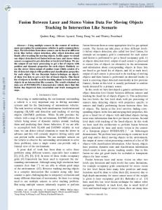
The primary contribution of this paper is the development of the patchlet surface element as a fundamental sensor primitive for stereo vision data. The idea of the patchlet arose from the observation that correlation stereo vision is a region matching technique and consequently senses surface patches, not points. The surface patch corresponds to the portion of the scene that falls within the neighbourhood of a given stereo pixel, as defined by the stereo matching algorithm, (typically a square image mask of 5 × 5 pixels.) The justification of this observation is given in Figure 4. As shown in Figure 4(a), when a single continuous surface covers the image neighbourhood, there is a high correlation of the image regions between the stereo cameras. Conversely, as shown in Figure 4(b), if there is a surface discontinuity within the image neighbourhood, there is little correlation between the images and consequently we can expect the stereo algorithm to fail. Since correlation stereo senses surface patches, a surface element representation for the sensor data is appropriate. One patchlet is generated for each valid pixel in the stereo image. The size of the patchlet is determined by projecting

Right Camera

Figure 3: Stereo error model Estimation errors are slight miscalculations in the disparity value due to local disturbances such as image noise. Matthies and Grandjean showed that these errors can be modeled successfully with a Gaussian distribution [MG94]. We used the estimation error model illustrated in Figure 3. Each disparity pixel from the stereo rig can be converted to a 3D point based on the projective camera equations: x u = ; f z

v y = ; f z

z B = f d

(1)

where (u, v) is the position of the disparity pixel in the reference camera image plane, (x, y, z) is the position of the observed 3D point in the reference camera coordinate frame and d is the pixel disparity. We define our sensor model error to be the combination of two parts: pointing error (p) 3

selected the Fisher [Fis53] distribution which is specially tailored for circular or spherical spaces. The Fisher distribution probability density function takes the form:

Surface Surface Right observation Left observation

Left Camera

Right Camera

Left Camera

(a) Continuous surface

P (x|µ, κ) =

κeκψ 4π sinh(κ)

(5)

where x is a given vector, µ is the distribution mean vector and κ is the Fisher confidence measure. ψ is the angular difference between µ and x. The Fisher confidence measure κ can be considered as the inverse of the standard deviation in Gaussian distribution.

Right Camera

(b) Discontinuous surface

Figure 4: Surface continuity and correlation stereo Confidence Cone

4.1. Patchlet creation

Z

To extract a patchlet at a particular location in the disparity image we use the neighbourhood around that location in the disparity image to estimate a local planar fit. We chose a square neighbourhood of the equal or smaller size as the stereo correlation mask (for experiments in this paper, we used a support region of 5 × 5 pixels). The steps of the patchlet creation are:

Y X size

Y size Origin

X Z variance

Figure 5: The Patchlet model

1. Determine 3D points from the disparity pixels 2. Find the best-fit plane.

the pixel onto the sensed surface. This projection distorts the patchlets so that they form a complete coverage over the imaged surface, however the patchlets are not uniform in size and shape. Patchlets that are farther from the camera will be larger and have higher uncertainty measures than close patchlets. Patchlets on oblique surfaces will be long and narrow rectangles, while patchlets on frontal-parallel surfaces will be square. Figure 5 illustrates the patchlet model. Each patchlet has its own coordinate system that defines its normal direction, its position in the world coordinate system, and the primary axes of its size parameters. The grey regions in the figure show the regions of uncertainty associated with the position and orientation parameters. Symbolically a patchlet is represented by the letter P and its parameters are:

3. Find the patchlet origin, coordinate frame and size. 4. Propagate confidence measures. These steps are elaborated below. 4.1.1 Determine 3D points We generate the 3D points, X = {X1 · · · Xn }, associated with the disparity pixels within the neighbourhood using (1). Each 3D point also has an independent covariance matrix, Λi , determined by (2), (3) and (4). 4.1.2 Find best-fit plane We find the best plane in a least-squares sense to X. Since each point has its own covariance matrix and these matrices are not aligned, we required an iterative solution. We selected Levenberg-Marquardt [PTVF92] as an efficient and robust optimisation approach. The error that is minimised is the Mahalanobis distance,

XP the patchlet 3D position in the world coordinate frame; ψP the patchlet normal vector; TwP the 4 × 4 homogenous transform that defines the patchlet’s local coordinate system; HP patchlet height (size in local Y );

ˆi )0 Λ−1 (Xi − X ˆi ) e2i = (Xi − X i

WP patchlet width (size in local X);

(6)

where Xˆi is the point on the current plane estimate that minimises the error ei . Xˆi is not necessarily the perpendicular projection of Xi onto the plane since the error term includes the covariance matrix Λi . ˆi we perform a whitening or sphering To determine X transform [KWV95] to both Xi and the plane estimate. In ˆi is the perpendicular projection of Xi the whitened space, X

ΛP the positional variance in normal direction; κP the confidence in the normal direction. The positional uncertainty is modeled using a Gaussian distribution with variance ΛP . The normal direction space is a two-dimensional sphere that wraps around on itself. Consequently, the Gaussian model is unsuitable. Instead we 4

onto the plane. Xˆi is determined in the whitened space and ˆi . After then the reverse transform is applied to determine X the Levenberg-Marquardt minimisation has converged, typically in 3 - 4 iterations, the plane normal direction ψP is obtained.

sentation of vectors that appears at pitch = ±π, (the “north” and “south” pole of the system). As well, placement of the origin at the centroid of the point set ensures the greatest independence between the angles and position ([Mur04] discusses angle and offset parameter independence). For our 3-parameter plane, {θ, φ, o} (where θ = yaw, φ = pitch and o = positional offset) the resulting covariance matrix is 3 × 3. The upper-left 2 × 2 submatrix is the covariance matrix, Λθφ , of the angles {θ, φ} and the lower-right value is ΛP , the variance of offset parameter o. κP is extracted from Λθφ by determining the direction of maximum variance and calculating the corresponding Fisher spherical confidence measure.

4.1.3 Find the patchlet origin, coordinate frame and size Each patchlet has its own coordinate system. The patchlet origin represents its centre position. The Z axis is the surface normal. For simplicity, we choose to represent patchlets as simple rectangles, rather than as the quadrilateral that is the projection of a square pixel onto an arbitrary surface. We select the X axis to be the larger primary axis of the rectangle and the Y axis the shorter. The Z axis, or plane normal, is already determined in the previous step. The patchlet origin, XP , is the projection of the disparity pixel centre onto the planar surface based on the camera parameters. We determine the X and Y axes by finding the major and minor axes of the ellipse that is the projection of a circular pixel onto the planar surface. This is determined by Y = Z × R and X = Y × Z where R is the unit vector associated with the ray that connects the reference camera projective centre with the patchlet origin. After the three coordinate axes and the origin are obtained, the world-to-patchlet transform TwP can be generated. The size in the patchlet Y axis direction, HP , is determined by the frontal-parallel pixel size which is HP = fz where z is the z coordinate value of the patchlet origin in the camera coordinate system and f is the camera focal length. The size in the patchlet X axis direction, WP , is determined HP by WP = cos α where α is the angular difference between the normal and the vector R.

5. Patchlet results Figure 6 shows the patchlet cloud generated from the stereo image given in Figure 6. The patchlets are rendered from two novel viewpoints to illustrate the quality of the depth reconstruction. In the left images, each patchlet is displayed with the greyscale of associated pixel in the reference image. In the right images, each patchlet is coloured white and Gouraud shaded. Each patchlet is the size of the pixel from which it was generated, projected onto the sensed surface. The patchlets are drawn at 90% of their full size so that the gaps between patchlets are easily visible.

4.1.4 Propagate confidence measures The last step in patchlet creation is the propagation of the uncertainty associated with the underlying 3D points to the patchlet parameter space. This determines the confidence parameters for the normal direction and patchlet position. The covariance matrix for the patchlet parameters can be determined by Λ = (J T J)−1 where J is the Jacobian ma∂ei . ei is the distance off the plane trix defined by Jij = ∂h j associated with point i as given in (6) and hj is the j th parameter of the plane. For our plane representation we use three parameters - yaw, pitch and distance from the origin. We evaluated J numerically by performing small perturbations of h and observing the resultant changes in e. Before evaluating J, we first transform the coordinate system so that the plane has yaw and pitch of 0 and the origin is centred at the pointcloud centroid. This moves the system as far as possible from the singularity of a polar-coordinate repre-

(a)

(b)

(c)

(d)

Figure 6: Patchlets rendered from two views : (a) and (c) are colored by the source image, (b) and (d) are white with Gouraud shading 5

Figure 7 gives a reference/disparity image pair similar to Figure 2, this time of an outdoor scene. The distances are larger than in Figure 2 and consequently the errors are greater, especially for farther regions of the image such as the staircase balustrade. Figure 8 shows the generated patchlet cloud rendered from a novel viewpoint. One can see in that there is considerable wobble in the represented surface due to stereo estimation errors. Figure 9 shows two additional views of the patchlet cloud. Figure 9(a) shows the balustrade viewed from the front of the steps. Significant smoothing between the steps and the balustrade can be seen. This is caused by the stereo correlation mask during the correlation algorithm.

Figure 1 (on first page) shows a close-up view of the foreground subject. In this view the individual patchlets are clearly visible. One can see that patchlets on more oblique surfaces, such as the lower cheek, are considerably larger in order to cover the entire surface continuously. There is some smoothing of features caused by the plane-fitting process of patchlet creation, but most observed smoothing (such as between the lower nose and the upper lip) is actually caused by the correlation stereo and is observable in the underlying point cloud.

(a) Reference image

(a) Far side of stairs

(b) Disparity image Figure 7: Stereo scene and disparity image of outdoor steps (b) Close up Figure 9: Scene rendered from additional viewpoints

5.1. Accuracy analysis The pointing accuracy required by (2) is supplied by the calibration process of the stereo camera. In our case it was supplied as a standard deviation of 0.03 pixels when operating with 320 × 240 resolution stereo images. However, the matching accuracy, m, is a feature of the correlation algorithm and is less straightforward to estimate. We derived the matching accuracy experimentally. To determine the matching accuracy we took a stereo image of a well textured planar surface (in this case, carpet

Figure 8: Patchlets generated from scene in Figure 7 and rendered from a novel viewpoint, Gouraud shaded 6

90

Y x 103 80

Unit Gaussian Matching Error 0.04 Matching Error 0.05 Matching Error 0.06

1.8000 1.7000 1.6000

70

1.5000

60

1.4000 50

1.3000 1.2000

40

1.1000 1.0000

30

0.9000 0.8000

20

0.7000 10

0.6000 0.5000

0

0.4000

0

0.5

1

1.5

2

2.5

3

3.5

0.3000 0.2000

Figure 11: Verification of patchlet accuracy: displayed is the histogram of Mahalanobis distances for normal direction of a patchlet cloud from its generative plane, overlaid with a Unit Gaussian. The Y axis is number of patchlets, the X axis is in standard deviation.

0.1000 0.0000 X 0.0000

1.0000

2.0000

3.0000

4.0000

5.0000

Figure 10: Determination of stereo matching accuracy: displayed is the histogram of Mahalanobis distances for three matching errors overlaid on the histogram expected from the Unit Gaussian. The Y axis is number of points, the X axis is in standard deviation.

beit with a slightly heavier tail.

6. Range image segmentation Patchlets were originally conceived as a tool for interpretation of stereo range data for mobile robot navigation. Mobile robots can collect a large amount of data from their environments, and a compact representation of the environment is desirable for mapping and navigation algorithms.

over a concrete floor). We then postulated several values for the matching error and evaluated their accuracy. Given the manufacturer-specified pointing accuracy and a hypothesis for the matching accuracy, we calculated the covariance matrix, Λx , for each disparity pixel in the stereo image as given by (3), as well as the disparity pixel’s x, y, z location. We then generated a normalized histogram of the Mahalnobis distance of each calculated 3D location from the plane. The histogram that best matched the Unit Gaussian would be the one with the accurate value for the matching error, (i.e., we iterated through a set of matching errors, searching for the one in which exactly 67% of the 3D points were within one standard deviation of the plane, 95% were within two standard deviations and so on.) The results of this search are shown in Figure 10. This test verifies two issues. First, that the histogram shape conforms to a Gaussian, verifying that the assumption of a Gaussian distribution for sensed data points is accurate. Second, it determines that a matching accuracy of 0.05 pixels standard deviation best modeled our system. As a sanity test, we then performed a regression test on the confidence measures for the patchlets created from the same planar surface scene. We used the pointing and matching errors as determined above, generated patchlets based on the resulting sensor model, and examined the histogram of the angular difference between the patchlet normals and the plane normal, normalised by the orientation confidence measure. The resulting histogram is displayed in Figure 11. The dashed line represents the unit Gaussian, our expected histogram level. The solid line represents the obtained histogram, which matches the Unit Gaussian very closely, al-

Figure 12: Surface segmentation Figures 12 and 13 show the results of probabilistic planar surface segmentation from the patchlet cloud from Figure 7 using clustering. The details of the segmentation process are described fully, and more complete results are presented, in [ML]. The method use ExpectationMaximisation to maximise the joint probability of the patchlet data and the segmented surfaces. Figure 12 uses the full patchlet model and includes dimensions for both surface normal and surface connectivity. Figure 13 gives the results of the clustering using only the patchlet position information. We can see from these figures that the added dimensionality of normal direction, surface contiguity and 7

References [CK]

Rodrigo Carceroni and Kiriakos Kutulakos. MultiView scene capture by surfel sampling: From video streams to Non-Rigid 3D motion, shape & reflectance. In ICCV 2001, pages 60–67.

[Fau93]

O D. Faugeras. Three-Dimensional Computer Vision: A Geometric Viewpoint. MIT Press, 1993.

[Fis53]

R.A. Fisher. Dispersion on a sphere. Proceedings of the Royal Society London, A127:295–305, 1953.

[Fua93]

P. Fua. A parallel stereo algorithm that produces dense depth maps and preserves image feature. Machine Vision and Applications, 6:35 – 49, 1993.

[Fua96]

P. Fua. Reconstructing complex surfaces from multiple stereo views. In Proceedings of the Fifth International Conference on Computer Vision (ICCV ’96), pages 1078 – 1085, Cambridge, Massachusetts, USA, June 1996.

7. Conclusions

[GD98]

J. Grossman and W. Dally. Point sample rendering. In Eurographics Rendering Workshop, 1998.

Point-based methods are gaining popularity in the graphics community for their ability to handle complex shapes without constructing or maintaining explicit connectivity between points. Stereo vision is a sensing technology that has considerable promise, it is inexpensive, fast and simple. In our research we are bringing these two areas together, demonstrating that point-based data primitives are a natural and useful way to interpret stereo vision 3D data. Stereo vision is a noisy sensor, consequently maintaining uncertainty data is a requirement for later shape analysis and especially important if one wishes to merge data from multiple viewpoints. Patchlets, our primitives, may be used directly for modeling as well as for data-driven shape analysis. We have demonstrated this usefulness through application to larger surface extraction and estimation.

[KWV95]

J. Karhunen, L. Wang, and R. Vigario. Nonlinear PCA type approaches for source separation and independent component analysis. In ICNN-95, Perth, Western Australia, November 1995.

[LW85]

M. Levoy and T. Whitted. The use of points as display primitives. Technical Report TR 85-022, The University of North Carolina at Chapel Hill, Department of Computer Science, 1985.

[MG94]

L. Matthies and P. Grandjean. Stochastic performance modeling and evaluation of obstacle detectability with imaging range sensors. Robotics and Automation (RA), 10:783–792, 1994.

[ML]

D. Murray and J. Little. Surface segmentation from stereo scenes. In 3DPVT 2004.

[Mur04]

D. Murray. Patchlets: a method of interpreting correlation stereo 3D data. PhD thesis, University of British Columbia, Vancouver, Canada, 2004.

[PTVF92]

W. H. Press, S. A. Teukolsky, W. T. Vetterling, and B. P. Flannery. Numerical Recipes in C : The Art of Scientific Computing. Cambridge University Press, 1992.

Figure 13: Segmentation using point information only proper weighting with the uncertainty measures greatly improves the quality of the segmentation.

7.1. Future work A stereo image is quite limited in its ability to reconstruct scenes due to its viewpoint limitation. For more complete models it is necessary to register views and combine the resultant 3D data. The uncertainty measures of patchlets make it well suited for the process of combining data. The certainty and the sizes of the patchlets can play and important role in maximising the accuracy of the final result. We are working to extend the application of patchlets to the combination of multi-viewpoint data. As well, the example application in this paper is restricted to extracting planar surfaces. This application was designed for constructing environment models of indoor environments for mobile robots, in which the planar surface constraint is largely accurate. However, for more complex and organic environments or objects, expanding the shape analysis to higher order parameterised surfaces would be advantageous.

[PZvBG00] H. Pfister, M. Zwicker, J. van Baar, and M. Gross. Surfels: Surface elements as rendering primitives. In Kurt Akeley, editor, Siggraph 2000, Computer Graphics Proceedings, pages 335–342. ACM Press / ACM SIGGRAPH / Addison Wesley Longman, 2000.

8

[SB98]

R. Sara and R. Bajcsy. Fish-scales: Representing fuzzy manifolds. In Proceedings of the 6th IEEE International Conference on Computer Vision (ICCV ’98), pages 811–817, 1998.

[ST92]

R. Szeliski and D. Tonnesen. Surface modeling with oriented particle systems. Computer Graphics, 26(2):185–194, July 1992.