Simultaneous Localization and Mapping with Stereo Vision - CiteSeerX

Simultaneous Localization and Mapping with Stereo Vision Matthew N. Dailey

Manukid Parnichkun

Computer Science and Information Management Asian Institute of Technology Pathumthani, Thailand Email: [email protected]

Mechatronics Asian Institute of Technology Pathumthani, Thailand Email: [email protected]

Abstract— In the simultaneous localization and mapping (SLAM) problem, a mobile robot must build a map of its environment while simultaneously determining its location within that map. We propose a new algorithm, for visual SLAM (VSLAM), in which the robot’s only sensory information is video imagery. Our approach combines stereo vision with a popular sequential Monte Carlo (SMC) algorithm, the Rao-Blackwellised particle filter, to simultaneously explore multiple hypotheses about the robot’s six degree-of-freedom trajectory through space and maintain a distinct stochastic map for each of those candidate trajectories. We demonstrate the algorithm’s effectiveness in mapping a large outdoor virtual reality environment in the presence of odometry error. Keywords—Localization, mapping, stereo vision, RaoBlackwellised particle filter, visual landmarks

I. I NTRODUCTION Simultaneous Localization and Mapping (SLAM) is the problem of a mobile robot constructing a metric map from noisy sensor readings while simultaneously estimating its location from the partial map and noisy odometry measurements. SLAM is one of the fundamental challenges for mobile robotics research. Altough recent years have seen great advances in 2D mapping with laser range finders, exclusively vision-based SLAM (VSLAM) is still limited to relatively small scale, highly structured indoor environments. We are interested in taking VSLAM beyond the typical office building environment into larger, but still structured, environments such as college campuses, office parks, and shopping malls. Potential application areas include security, inspection, landscape maintenance, agriculture, and personal service. Achieving this goal without giving the robot an a-priori map requires new technology. The majority of vision-based SLAM research to date has focused on automatic construction of occupancy grids or topological maps (see [8] for a survey), both of which are inappropriate for large-scale metric mapping. The ideal approach would construct a sparse 3D representation of the environment. Early VSLAM systems did use sparse features, but they typically compressed the map to 2D. For example, Kriegman, Triendl, and Binford’s system [11] uses a stereo sensor to extract vertical lines from the environment. Observed lines are used to reduce odometric uncertainty using an extended

c 2006 IEEE 1–4244–0342–1/06/$20.00

Kalman filter (EKF), then the observations are in turn used to update an environment map containing 2D point features representing the observed vertical lines. Yagi, Nishizawa, and Yachida’s system [21] took a similar approach but used a single omnidirectiona vision sensor and accumulation of measurements over time, rather than stereo, to determine the positions of vertical line landmarks. These systems and others have amply demonstrated the efficacy of VSLAM based on line landmarks in constrained indoor environments with smooth floors. Faugeras and colleagues [1], [22] were the first to develop a VSLAM system storing a sparse 3D map. Their system first constructs a “local” 3D line segment map of the current scene using trinocular stereo. It explicitly represents the uncertainty about each feature’s robot-relative pose in the form of a covariance matrix. The new local map is registered against the current global map and used to update an estimate of the robot’s position using an EKF. Finally, assuming the robot’s position, the global map is be updated with the freshly observed features, again using EKFs. Se, Lowe, and Little [16] demonstrate the use of SIFT (scale invariant feature transform) point features as landmarks for the VSLAM problem. Their system also uses a trinocular stereo camera rig and models the positional uncertainty of the landmarks with Kalman filters. Sim and Dudek [17] take a different approach; rather than prespecifying the features (lines, points, corners, and so on) that should be used for map building and localization, their system learns generative models for the appearance of salient features during exploration. Until quite recently, most VSLAM systems limited themselves by separating the motion estimation and map estimation problems. Typically, at each step, the robot’s location would be estimated via Bayesian inference or some other estimation technique, then that position would be assumed for the map update. While this approach leads to fast algorithms, not considering alternative robot poses when estimating landmark positions is suboptimal. Other researchers in the robotics community took a formal probabilistic approach and explored the possibility of representing, at each point in time, the full joint posterior distribution over robot trajectories and landmark

ICARCV 2006

positions. Smith, Self, and Cheeseman [19] introduced the “stochastic map,” which represents not only the positions of landmarks in the world with their associated uncertainties, but also the uncertainty of the robot’s position, the covariance between each pair of landmarks, and the covariance between the robot’s position and each landmark. This seminal theoretical work inspired many successful SLAM systems, e.g. [2], [7], [12]. In a particularly impressive demonstration of the power of the stochastic map approach, Davison and colleagues [5], [6] have solved the VSLAM problem with point landmarks extracted from a single camera without odometry. Their system runs in real time at 30 Hz. While the stochastic map very accurately represents all of the available information about landmark and robot positions (within the limits of the Gaussian approximation), the method unfortunately cannot scale to the thousands of landmarks needed for large-scale environments, due to the size of the full covariance matrix. Murphy [13], however, recognized that in SLAM, map elements are conditionally independent given the robot’s trajectory through time. He used this insight in the design of the Rao-Blackwellised particle filter (RBPF), in which the joint posterior over robot trajectories and maps is represented by a set of samples or particles, each particle containing one possible robot trajectory and the corresponding stochastic map. The fact that the robot’s trajectory is fixed for a given particle has an important consequence: all of the covariances between different map elements in the stochastic map become 0. For a landmark map, this means the covariance matrix for each individual landmark is sufficient to represent all of the available knowledge of the environment. Murphy only demonstrated the RBPF on a toy problem, but more recent work has applied the technique to the real world with immense success. Montemerlo, Thrun, and colleagues [20] use the RBPF and 2D point landmarks measured by a laser scanner to construct large-scale 2D maps. In their system, each particle represents a possible robot trajectory, set of data associations, and landmark map. The maps are stored in a tree structure that allows sharing subtrees between particles, allowing a real-time implementation that scales to thousands of landmarks. Eliazar and Parr [9] also use the RBPF and a laser scanner for SLAM, but build a 2D occupancy grid rather than a landmark database. Their algorithm also requires a sophisticated data structure that allows sharing maps between particles. Even more recently, researchers have begun to apply the RBPF to the VSLAM problem. Sim et al. [18] extract SIFT point features from stereo data and combine the observations with visual odometry to build 3D landmark maps. According to the authors, this state-of-the art system has constructed the largest and most detailed VSLAM map ever, in a large indoor laboratory environment. In our work, we take a similar approach, combining the RBPF with vision sensors, except that we use 3D line segments for localization and map building, rather than the more commonly used point features [18], [20]. Line parameters can

be estimated more accurately than points, since the estimate incorporates more observed data. This means it may be possible to obtain more accurate robot localization from line landmarks than point landmarks, depending on the characteristics of the robot’s workspace. Lines also provide more information about the environment’s geometry than do points, allowing more sophisticated inference about the structure of the world. However, lines also have an important disadvantage with respect to points: they are less distinctive, making it more difficult to find correct correspondences between a set of observed lines and the lines in a stored model. We overcome this difficulty by sampling many possible poses from the robot’s motion model, obtaining a different possible observation-model correspondence given each robot pose, and allowing the “fittest” correspondences to survive in the particle filter. Our algorithm is called VL-SLAM (Visual Line-based SLAM). Here we describe VL-SLAM and demonstrate its effectiveness in a series of experiments. The main contributions of this paper are 1) an effective sensor model for line landmarks obtained from a stereo camera rig, 2) a new proposal distribution for the RBPF that overcomes the limitations imposed by highly uncertain correspondences, and 3) experimental evidence of the feasibility of VL-SLAM using realistic, albeit synthetic, data. II. VL-SLAM VL-SLAM is based on the “FastSLAM” family of algorithms proposed by Montemerlo, Thrun and colleagues [20]. At each point t ∈ 1 . . . T , the robot performs an action ut taking it from position st−1 to st and uses its sensors to obtain an observation zt . We seek a recursive estimate of p(s0:t , Θ | u1:t , z1:t ) where Θ is a map containing the positions of each of a of point landmarks. Rather than estimate the distribution analytically, we approximate the posterior with a discrete of Mt samples (sometimes called particles) o n [m] [m] < s0:t , Θ0:t >, where each index m ∈ 1 . . . Mt .

(1) set (1) set (2)

[m]

Here s0:t is the specific robot trajectory from time 0 to time t [m] associated with particle m, and Θ0:t is the stochastic landmark [m] map associated with particle m (the map is derived from s0:t , z1:t , and u1:t ). FastSLAM (and VL-SLAM) use the sequential Monte Carlo techniques of sequential importance sampling and importance resampling. First, for each particle, we sample from some proposal distribution π(s0:t , Θ0:t | z1:t , u1:t )

(3)

to obtain a temporary set of particles for time t, then evaluate the importance weight w[m] for each temporary particle, where w(s0:t , Θ0:t ) =

p(s0:t , Θ0:t | u1:t , z1:t ) . π(s0:t , Θ0:t | u1:t , z1,t )

(4)

The importance weights are normalized to sum to 1, then we sample Mt particles, with replacement, from the temporary particle set according to the normalized weights.

VL-SLAM extends FastSLAM with a new sensor model for 3D line segments and a new proposal distribution π(·) appropriate for environments with highly ambiguous observationmodel correspondences. We first describe the 3D line segment sensor model then VL-SLAM proposal distribution. A. VL-SLAM 3D Line Segment Sensor Model After each robot motion ut , a set of trinocular stereo images is captured, and a set zt of landmark measurements (line segments) is extracted from those images. These line segment measurements, along with the measured motion ut , are used to update each particle’s map and position estimate. Our system assumes a calibrated stereo camera rig with three pinhole cameras. It can handle general fundamental matrices (the images need not be perfectly rectified), but we do assume that one camera is roughly horizontally displaced and a second camera is roughly vertically displaced from a third (reference) camera. The basic 2D feature in our system is the line segment. We extract line segments using Canny’s method [4] following the implementation in VISTA [14]. The edge detector first performs nonmaxima suppression, links the edge pixels into chains, and retains the strong edges with hysteresis. Once edge chains are extracted from the image, we approximate each chain by a sequence of line segments. Short line segments, indicating edges with high curvature, are simply discarded in the current system. We use a straightforward stereo matching algorithm similar to the approach of [22]. For each line segment in the reference image, we compute the segment’s midpoint, then consider each segment intersecting that midpoint’s epipolar line in the horizontally displaced image. Segments not meeting line orientation and disparity constraints are discarded. Each of these potential matches determines the location and orientation of a segment in the third image. If such a consistent segment is indeed found in the third image, the potential match is retained; otherwise it is discarded. If at the end of this process, we have one and only one consistent match, we assume it correct; otherwise, the reference image line segment is simply ignored. Now our goal is to estimate a three-dimensional line from the three observed two-dimensional lines. Infinite lines have four instrinsic parameters, so it would make sense to use a four-dimensional representation of a lines. However, since VL-SLAM uses a Kalman filter to combine landmark observations, we require a linear parameterization of landmarks, and no linear four-dimensional representation of lines exists [1]. Instead we represent lines with six components: a 3D point representing the midpoint of the observed line segment and a 3D vector whose direction represents the direction of the line and whose length represents the distance from the line segment’s midpoint to one of its endpoints. This 6D representation behaves well under linear combination, so long as the direction vectors are flipped to have a positive dot product. First we obtain a maximum likelihood estimate of the infinite 3D line’s parameters assuming Gaussian measurement

error in the image using Levenberg-Marquardt minimization [15]. As an initial estimate of the line’s parameters, we use the 3D line (uniquely) determined by two of the 2D line segment measurements. Once the infinite line has been estimated, we find the segment’s extrema and midpoint using the observed data. Through each step of the 3D line estimation process, we maintain explicit Gaussian error estimates. We begin by assuming spherical Gaussian measurement error in the image with a standard deviation of one pixel. Arranging the n (x, y) coordinates of the pixels in a line as a column vector x, the covariance of x is simply Σx = I2n×2n . Since the vector of parameters l describing the 2D line best fitting x is a nonlinear function l = f (x), the covariance of l is Σl = JΣx J T , where ∂f J is the Jacobian matrix ∂x evaluated at x. The maximum likelihood estimate of the 3D line obtained from the three 2D line segments l = (l1 , l2 , l3 ) is clearly not a simple function, since it is computed by an iterative optimization procedure. However, if l = f (L) is the function mapping from the parameter space to the measurement space, ˆ is a random variable with it turns out that, to first order, L T −1 covariance matrix (J Σl J) , where J is the Jacobian matrix ∂l ∂L [10]. The rank of the resulting covariance matrix is only four, however, so to constrain the remaining two degrees of freedom, we add to the rank-deficient covariance matrix a covariance matrix describing the expected error in our estimate of the segment’s midpoint and another covariance matrix describing the expected error in our estimate of the segment’s length. This gives us a full-rank covariance matrix that restricts matching line segments to not only be similar in terms of their supporting infinite line, but also to overlap and have similar length. Once the six-dimensional representation of an observed 3D line is estimated from a trinocular line correspondence, it is necessary to transform that line from camera coordinates into robot coordinates, since the reference camera is in general translated and rotated relative to the robot itself. It is also necessary to transform landmarks from robot coordinates into world coordinates, when the robot’s position is determined, for instance, and from world coordinates back to robot coordinates, when a landmark in the map is considered as a possible match for an observed (robot coordinate) landmark. In each of these cases, the transformed line L0 = t(L) is computed as a nonlinear function of the original line, and the transformed line’s covariance is propagated by ΣL0 = JΣL J T , where J is ∂t the Jacobian matrix ∂L evaluated at L. B. VL-SLAM Proposal Distribution The proposal distribution π(·) (3) can be any distribution that is straightforward to sample from. However, it is best if π(·) closely approximates the full joint posterior (1), in which case the importance weights will be nearly uniform, and most particles will “survive” the resampling step. In FastSLAM 1.0 [20], the proposal distribution is simply p(st | st−1 , ut ), i.e. the motion model predicting st given a previous position st−1 and action ut . The authors observe that this proposal distribution,

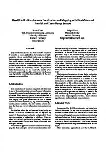
(a) Fig. 1.

(b)

(c)

Sample trinocular image set captured in simulation. (a) Reference image. (b) Horizontally aligned image. (c) Vertically aligned image.

while simple to sample from, does not take into account the current observation zt . This leads to FastSLAM 2.0, in which [m] [m] the proposal distribution is p(st | s0:t−1 , Θ0:t−1 , u1:t , z1:t ). This distribution takes not only the previous robot pose st−1 and current action ut into account, but also considers the current map Θ0:t−1 and new observation zt . In the general case, this distribution could be quite difficult to sample from, but the authors find that by linearizing the sensor model and applying the Markov assumption, the proposal distribution can be approximated to first order by a Gaussian distribution whose mean and covariance can be calculated from known quantities, if the correspondence between the observation zt and the current map Θ0:t−1 is known. When the correspondences are unknown (the usual case in SLAM), FastSLAM 2.0 assumes the maximum likelihood correspondence or draws a sample from a probability distribution over all possible correspondences. When the observations and landmarks are sparse, as is the case in the FastSLAM environment, this is straightforward, and FastSLAM 2.0 is much more successful than FastSLAM 1.0, since it uses the available set of particles wisely [20]. In VL-SLAM, however, each observation consists of on the order of 100 individual 3D line segments, and typically the landmark database contains several potential matches for each observed line. This means that it is impossible to consider even a small fraction of the possible correspondences for each particle. In practice, to limit the computational complexity, we must draw a single correspondence from the set of all possible correspondences without considering too many alternatives. But how can we choose a likely correspondence for a given observation? In VL-SLAM, when propagating a particle forward from time t − 1 to time t, we first fraw a sample s0t from the robot’s motion model to establish a correspondence between the observed line segments and the current map (resembling FastSLAM 1.0), then from that intermediate sample point, assuming the established correspondence, sample again, from the FastSLAM 2.0 proposal distribution. As in FastSLAM 2.0, the proposal distribution is closer to the full joint posterior distribution, concentrating more of the temporary particles in regions of high probability according to the full joint posterior. To calculate the importance weights for the the VL-SLAM proposal distribution, we first introduce random variables nt

indicating the correspondence between the line segments observed at time t and the map. In VL-SLAM, the mth particle’s [m] map Θ0:t is a deterministic function of the sampled trajectory [m] [m] s0:t , the sampled correspondences n1:t , and the observations z1:t , so we rewrite the desired full joint posterior as p(s0:t , n1:t | u1:t , z1:t ).

(5)

Now, assuming we have a good estimate of the full joint posterior at time t − 1, the VL-SLAM proposal distribution can be written as the product [m]

[m]

0[m]

| nt , st

p(st

[m]

[m] 0[m] [m] s0:t−1 , n1:t−1 , z1:t−1 , u1:t )× [m] [m] 0[m] p(st | s0:t−1 , n1:t−1 , z1:t−1 , u1:t )× [m] [m] p(s0:t−1 , n0:t−1 | u1:t−1 , z1:t ),

[m]

p(nt

[m]

, s0:t−1 , n0:t−1 , z1:t , u1:t )×

| st

(6)

where s0t represents the intermediate sample drawn from the motion model. For the mth particle, the importance weight is the ratio of the expressions in (5) and (6), which, with several applications of Bayes’ rule and the Markov assumption, can be closely approximated as (details ommitted): [m]

wt

= [m]

p(st [m]

p(st

0[m]

| zt , s t

[m]

[m]

[m]

| st−1 , ut )p(zt | s0:t , n1:t , z1:t−1 ) [m]

[m]

0[m]

, n1:t , s0:t−1 , z1:t−1 , u1:t )p(st

[m]

| st−1 , ut ) (7)

Following [20], we linearize the sensor model and motion model, which leads to straightforward Gaussian approximations for each of the terms in (7). Except for the sensor model and proposal distribution just described, VL-SLAM is similar to FastSLAM (see [20] for details). Once correspondences and the sampled pose are determined for an individual particle, each observed landmark is combined with its corresponding map landmark using an extended Kalman filter, or initialized as a new landmark in the map. To achieve fast search for landmarks corresponding to a given observation, each particle’s map is stored in a binary kD tree whose leaves are the 3D line segments with associated Gaussian uncertainties. However, to minimize total memory requirements and to enable constant-time copying of maps

during the resampling stage, the particles are allowed to share subtrees. As we shall see in the next section, the diversity of possible correspondences introduced by the first sampling step (as in FastSLAM 1.0), combined with the use of the current observation zt in the proposal distribution (as in FastSLAM 2.0), allows VL-SLAM to outperform both FastSLAM 1.0 and FastSLAM 2.0 on a challenging synthetic testbed. III. E XPERIMENTAL R ESULTS To enable rigorous testing of VL-SLAM in an environment with a precisely known ground truth, we implemented a virtual reality simulation allowing a virtual robot to move through a virtual world rendered with OpenGL from a VRML model. We chose as an environment a publically-available 3D model of Housestead’s fort, a Roman garrison from the 3rd century A.D. on Hadrian’s Wall in Britain [3]. A sample view from our virtual trinocular stereo rig is shown in Figure 1. We teleoperated our virtual robot through this virtual world in a long loop of about 300m. At approximately 1m intervals, the virtual camera rig was instructed to capture a set of stills from its three cameras. The virtual camera models a real 10cm baseline, 70◦ field of view trinocular rig we recently built in our lab. To make the dataset somewhat challenging, we simulated the effects of a traveling on an imperfect outdoor surface, so that the robot’s vertical (Z) position varied approximately ±0.04m from 0, its pitch and roll varied ±2.5 degrees from 0, and its yaw varied ±3 degrees from its expected course. This environment is an interesting testbed for VL-SLAM because, on the one hand, it generates many long, strong, straight edges that should be useful for localization. On the other hand, it is highly textured, creating a large number of edges, and the textures are highly repetitive in many places, leading to many ambiguities for correspondence algorithms. It is also large enough to preclude fine-grained grid-based techniques and noisy enough to preclude the use of flat-earth or three-degree-of-freedom assumptions. We compared VL-SLAM with our own implementations of FastSLAM 1.0 and 2.0. As previously discussed, FastSLAM 2.0 was not designed to handle large observations with highly uncertain correspondences. In our implementation, we simply obtain the maximum likelihood correspondence assuming the [m] robot is at the position obtained by propagating st−1 forward [m] in time according to odometry to obtain sˆt . With this caveat about the FastSLAM 2.0 results, Figure 2 shows one measure of each algorithm’s performance: the log-likelihood of the observation data given the best particle’s robot trajectory sample and map; Figure 3 shows the final map according to the best VL-SLAM particle. All of the localization algorithms do much better than the baseline (odometry-only) algorithm. Due [m] to its commitment to robot position sˆt when determining correspondences in our implementation, FastSLAM 2.0 fares rather poorly. Since FastSLAM 1.0 samples from the motion model before obtaining a correspondence, it performs much better, but VL-SLAM, which combines the best features of both algorithms, outperforms them both.

IV. C ONCLUSION In this paper, we have demonstrated the feasibility of VLSLAM on a challenging synthetic data set. The VL-SLAM proposal distribution improves on FastSLAM in environments with large numbers of ambiguous observations. However, Figure 2 shows that there is still improvement to be made: the log-likelihood of the observations given perfect localization is still much better than the log-likelihood of the observations under VL-SLAM’s model. This means there is still information about the robot’s position to be exploited in the observed data. This is also evidenced in Figure 3, which compares the VLSLAM map to the map constructed with perfect knowledge of the robot’s location. Although the map is locally fairly accurate, global drift occurs throughout the run, preventing the algorithm from closing the loop when the robot returns to its starting position. This is most likely due to an impoverished set of particles. In future work, we plan to improve VL-SLAM’s loop closing behavior and evaluate the algorithm on a variety of indoor and outdoor real-world data sets. ACKNOWLEDGMENTS This research was supported by Thailand Research Fund grant MRG4780209 to MND. R EFERENCES [1] N. Ayache and D. Faugeras. Maintaining representations of the environment of a mobile robot. IEEE Transactions on Robotics and Automation, 5(6):804–819, 1989. [2] S. Borthwick and H. Durrant-Whyte. Simultaneous localisation and map building for autonomous guided vehicles. In Proceedings of the IEEE/RSJ/GI International Conference on Intelligent Robots and Systems (IROS), pages 1442–1447, 1994. [3] British Broadcasting Corporation. Housestead’s Fort (3D model), 2004. http://www.bbc.co.uk/ history/3d/houstead.shtml. [4] J. Canny. A computational approach to edge detection. IEEE Transactions on Pattern Analysis and Machine Intelligence, 8(6), 1986. [5] A. Davison. Real-time simultaneous localisation and mapping with a single camera. In Proceedings of the International Conference on Computer Vision (ICCV), pages 1403–1410, 2003. [6] A. Davison, Y. Cid, and N. Kita. Real-time 3D SLAM with wide-angle vision. In Proceedings of the IFAC Symposium on Intelligent Autonomous Vehicles, 2004. [7] A. Davison and N. Kita. 3D simultaneous localisation and map-building using active vision for a robot moving on undulating terrain. In Proceedings of the IEEE Conference on Computer Vision and Pattern Recognition (CVPR), pages 384–391, 2001. [8] G. DeSouza and A. Kak. Vision for mobile robot navigation: A survey. IEEE Transactions on Pattern Analysis and Machine Intelligence, 24(2):237–267, 2002. [9] A. Eliazar and R. Parr. DP-SLAM 2.0. In Proceedings of the IEEE International Conference on Robotics and Automation (ICRA), 2004. [10] R. Hartley and A. Zisserman. Multiple View Geometry in Computer Vision. University Press, Cambridge, UK, 2000. [11] D. Kriegman, F. Triendl, and T. Binford. Stereo vision and navigation in buildings for mobile robots. IEEE Transactions on Robotics and Automation, 5(6):792–803, 1989. [12] P. Moutarlier and R. Chatila. Stochastic multisensory data fusion for mobile robot location and environment modeling. In 5th International Symposium on Robotics Research, 1989. [13] K. Murphy. Bayesian map learning in dynamic environments. In Advances in Neural Information Processing Systems (NIPS), 1999. [14] A. Pope and D. Lowe. Vista: A software environment for computer vision research. In IEEE Conference on Computer Vision and Pattern Recognition, 1994. [15] W. Press, B. Flannery, S. Teukolsky, and W. Vetterling. Numerical Recipes in C. Cambridge University Press, Cambridge, UK, 1988.

Log Likelihood

-400

-600

-700

Fig. 2.

FastSLAM 1.0 FastSLAM 2.0 VL-SLAM Perfect localization Odometry only

-500

0

200

400

600

Number of particles

800

1000

Log likelihood of line observations according to the best particle’s sampled robot position and map, averaged over 320 sets of observations.

(a) Fig. 3.

(b)

Map constructed by VL-SLAM (a), compared to the the map assuming perfect knowledge of the robot’s trajectory (b).

[16] S. Se, D. Lowe, and J. Little. Mobile robot localization and mapping with uncertainty using scale-invariant visual landmarks. The International Journal of Robotics Research, 21(8):735–758, 2002. [17] R. Sim and G. Dudek. Learning generative models of scene features. International Journal of Computer Vision, 60(1):45–61, 2004. [18] R. Sim, P. Elinas, M. Griffin, and J. Little. Vision-based SLAM using the Rao-Blackwellised particle filter. In IJCAI Workshop on Reasoning with Uncertainty in Robotics (RUR), 2005. [19] R. Smith, M. Self, and P. Cheeseman. Estimating uncertain spatial relationships in robotics. In I. Cox and G. Wilfong, editors, Autonomous Robot Vehicles. Springer Verlag, 1990. [20] S. Thrun, M. Montemerlo, D. Koller, B. Wegbreit, J. Nieto, and E. Nebot. FastSLAM: An efficient solution to the simultaneous localization and mapping problem with unknown data association. Journal of Machine

Learning Research, 2004. To appear. [21] Y. Yagi, Y. Nishizawa, and M. Yachida. Map-based navigation for a mobile robot with omnidirectional image sensor copis. IEEE Transactions on Robotics and Automation, 11(5):634–648, 1995. [22] Z. Zhang and O. Faugeras. 3D Dynamic Scene Analysis. Springer-Verlag, 1992.