Pattern Recognition Based on Multidimensional Models Michal Haindl1,2, Pavel Pudil1, Petr Somol1,2 Faculty of Management, Prague University of Economics Jarošovská 1117/II, Jindřichův Hradec
[email protected] .cz 2 Inst.of Information Theory & Automation, Academy of Sciences CR Pod vodárenskou věží 4, 182 08 Praha 8
[email protected],
[email protected] 1
Annotation: This chapter explains general model-based approaches to several basic pattern recognition applications followed by a concise description of three fundamental multi-dimensional data model classes. For each model class a solution to parameter estimation and model data synthesis is outlined. Finally an overview of the strengths and weaknesses of studied multi-dimensional data model groups is given.
1
Introduction
Recognition and processing of multi-dimensional data (or set of spatially related objects) is more accurate and efficient if we take into account all interdependencies between single objects. Objects to be processed like for example multi-spectral pixels in a digitized image, are often mutually dependent (e.g., correlated) with a dependency degree related to a distance between two objects in their corresponding data space. These relations can be incorporated into a pattern recognition process through appropriate multidimensional data model. If such a model is probabilistic we can use consistent Bayesian framework for solving many pattern recognition tasks. Data models are simultaneously useful to specify natural constraints and general assumptions about the physical world and a data capturing process hence they are essential in many data modelling or analytical procedures such as classification, segmentation, discontinuity detection, restoration, enhancement and scene analysis in general. Features derived from multi-dimensional data models are information preserving in the sense that they can be used to synthesize data spaces closely resembling original measurement data space. Topological relations between objects are very often expressed by their indexation. Multi-dimensional data elements can be indexed (using multiindices r={r1, r2,…} ) on some regular finite or infinite lattices I, r∈I or even on completely irregularly distributed sites like vertices of some graph structure. Neighbourhood structures and indexation lattices can be even more complicated for higher dimensions and multiresolution data representations. Finite data lattices additionally require some assumption for their boundary conditions (e.g., free boundary conditions, toroidal boundary conditions, etc.) which can significantly influence the numerical efficiency of resulting
80
algorithms (e.g., Markovian models). In the case of usual colour image this vector has three components but multi-spectral images used in remote sensing applications can have tens of such components for every multispectral pixel vector and the underlying index lattice is three-dimensional. Digital video data have the additional time component thus a four dimensional index lattice is needed. Such large amount of data is difficult to analyse, store or transport. Efficient processing of large data sets requires an underlying model explaining dominant statistical characteristics present in these data. Finally an image interpretation is an example of data lattice with irregularly distributed sites. Mathematical multi-dimensional data models are useful for describing many of the multi-dimensional data types provided that we can assume some data homogeneity so some data characteristics are translation invariant. If this assumption does not hold, no advantage can be gained using data models for large data spaces like images. While the 1D models like time series are relatively well researched and they have rich application history in control theory, econometrics, medicine and many other recognition applications, multi-dimensional models are much less known and their applications are still limited. The reason is not only unsolved theory difficulties but mainly their huge computing power demands which prevented their wider use until recently. Several multi-dimensional data models may be thought of as a natural generalization of their 1D counterparts. However, in the nD domain, contrary to the 1D case, there is no natural order definition and hence terms like past or future are meaningless unless defined with respect to some specific and usually artificial order. Different order definitions in nD lead to different orthogonal decompositions. nD problems are also intrinsically different from 1D and consequently 1D models and techniques are not easily extended or transferred into the nD or even only to 2D world. Therefore a high quality goal in a nD space is better achieved by exploiting nD domains characteristics rather than imposing 1D ideas into nD. Dimensionality is another major difficulty. Many 1D calculation techniques can become intractable for small multi-dimensional data sets and for quite simple models.
2
Pattern Recognition Applications
It is possible to divide data models applications into two broad categories: synthesis and analysis. The frequent synthesis application is the missing data reconstruction. Another common application is texture synthesis. Analytical applications include data classifications or segmentation, data space directionality analysis, compression and some others. The popular discontinuity detection and image restoration problems can be seen as classification problems with two and K (number of measurements quantization levels) classes, respectively. Recognition applications in this chapter are demonstrated on images because they are illustrative and monospectral images require relatively simple 2D models. However the model-based approaches are general and can be used for any multi-dimensional data 81
recognition provided we are able to efficiently model the corresponding data spaces.
2.1
Contextual Classification
Classification solves the assignment of single objects (patterns) to one of . The commonly used several (K) prespecified categories context-free Bayesian or other decision rules for object (e.g., multi-spectral image pixels, letters, p7honemes, etc.) classification (classifiers) classify a single object using only this object's measurements (features) not using its possible mutual correlation with other objects in the segmented object space. It is well known that for example neighbouring image pixels are highly spatially correlated and similar relations hold also for other types of measurements. Such supervised (classification) or unsupervised (segmentation, clustering) algorithms neglect information from the classified object surroundings and thus inevitably deteriorate the classification error rate. Contextual classification solves the problem of estimating labels in true unobservable object set ω given the observation data sets (e.g., an image) Y. Let be the N-tuple random vector representing true labels . Let vector represent the site observations in the same ordering as is the d dimensional random vector representing measurements on the object at the site r. The standard context-free Bayes subsequently for all if decision rule assigns Yr to the class (1) Using the usual notion of discrimination function formulated as follows:
, a decision rule can be
Yr is assigned to the class if . The optimal contextual Bayesian decision rule, which minimizes the average mean loss of single decision problems of an object (deterministic decision function, zeroone loss function) [5], should use all attainable information from data: .
(2)
A solution of (2) is hardly a solvable task because of complicated posterior probability density and decision rule implementation. A practical classification scheme must be a compromise between information used and the computational complexity of an algorithm. The evaluation of the discrimination function (2) can be simplified by accepting some additional simplifying assumption. Usual Markovian simplification , where
denotes a neighbourhood of the site r such that
, (3)
82
is substantiated from the fact that for many indexed object sets (e.g., images) the class conditional correlation between single object's measurements drops more rapidly with their distance than the same unconditional correlation. Using some other simplifying assumptions (e.g., conditional statistical independence of objects indexed in Ir, knowledge of true classes of neighbouring objects) we can get the whole range [5] of possible contextual Bayesian classifiers. Statistical non Bayesian contextual classifiers can be derived similarly. The evaluation of statistical contextual classifiers discriminate functions requires appropriate simultaneous multi-dimensional probabilistic models such as the models described in the subsequent section 3. Classical image processing task of edge detection or more generally discontinuity detection in a multi-dimensional data space can be formulated also as a contextual classification problem with two site labels - edge, nonedge. Contextual techniques just described can be applied to it. The edge detection can be formulated as the estimation of an unobservable binary random field indexed on a dual lattice The dual lattice is defined to have its sites placed midway between each neighbouring pair of I sites. The indirect measurement field for the corresponding edge sites are observable measurements Y on the lattice I. A possible maximum a posteriori (MAP) solution is to maximize .
(4)
If we assume to be Gibbs random field (5) and measurements Y is conditionally independent on each other then also a Gibbs random field with the corresponding energy function [12].
2.2
Segmentation
The goal of data space segmentation is the abstraction of complex data space into a description comprising a relatively small number of labeled regions (e.g., Fig. 1). Every region is distinguished by homogeneous characteristics which are significantly different for each region to be discriminatory. The segmentation task can be formulated similarly as the restoration task to be a problem of recovering unobservable data from their degraded observable version. While for the restoration the goal is undegraded original data the segmentation goal is a segmentation map containing some class indicators. Segmentation of a data space in the absence of a priori information is very difficult and still generally an unsolved task. The main problem is that the model and its parameters are unknown before segmentation; however, to effectively estimate model parameters the segmentation itself is needed. The spatial models impose prior constraints on acceptable labellings through a priori probabilities, so highly connected labellings are favourably weighted. A data segmentation can be based on a data redundancy measure. A good unsupervised classification should be highly redundant with the original data space. Segmentation can be based on the MAP Bayesian estimator (4) where 83
can be a discontinuity map or a segmentation map. In the case of the discontinuity map we cannot decide if unconnected distant regions share similar characteristics. The labeling field model can be assumed to be a Markov random field (MRF) .
(5)
The MAP estimation minimizes the probability that any object in I will be misclassified. Alternatively the maximum marginal posterior probability, marginal posterior expectation, clustering or some other criterion can be used.
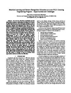
Figure 1. Colour textures mosaic and its segmentation based on a Markov random field model [8]
3
Multi-Dimensional Models
Several approaches to multi-dimensional data modelling exist, each of them has its advantages and also limitations. Existing models can be categorized using different criteria like deterministic and stochastic, causal and non causal, hierarchical and single-scale, syntactical and parametric, or another possible division is according to their primary modelling strength into low and high frequency subsets. Practical applications have models with solved parameter estimation step, different ad hoc models or models with unknown parameter estimation are useless for pattern recognition applications. Several different data models exist and random field models are among the most powerful and flexible ones, because choosing different neighbour sets and different types of probability distribution for the random variables a variety of distinct data space types can be generated. In the structural approach (Syntactic Models) a data set is considered to be defined by subpatterns which occur repeatedly according to a set of welldefined placement rules within the overall pattern. In order to model the data set of interest, it is necessary to have the stochastic tree grammar actually inferred from the available data samples. Such an inference procedure requires the inference of both the tree grammar and its production
84
probabilities. Unfortunately, a general inference procedure for stochastic tree grammars does not exist and is still a subject of research. The Markov random field (MRF) is a family of random variables with a joint probability density on the set of all possible realizations Y of the lattice I, subject to the positivity condition and some Markovianity condition (e.g. strict sense Markovianity). MRF parameter estimation (similarly also the MRF synthesis) is a complicated task even for single and simple MRF models. The complexity of estimation further increases for more than two-dimensional MRF models or if the neighbourhood system has to be simultaneously estimated. The complexity of posterior parameter distribution for most MRF models and possible parameter priors means that analytical Bayesian estimation is rarely possible - one of these exceptions is the causal Gaussian wide-sense Markov random field (CAR). Instead some Markov chain Monte Carlo method like the Gibbs sampler or the Metropolis algorithm has to be used. Multi-variate probabilistic mixtures models (MM) with components are defined as products of univariate discrete probability distributions. The unknown parameters of the approximating mixture can be estimated by means of the iterative EM algorithm [2], which maximizes the likelihood function. The advantageous property of the mixture models is easy computation of any univariate conditional distribution. The implementation of the EM algorithm is simple but time consuming and there are some well known computational problems, e.g., the proper choice of the number of components, the existence of local maxima of the likelihood function and the related problem of a proper choice of the initial parameter values. In some applications there might be problem to get sufficiently large learning set.
Summary Several possible models exist for multi-dimensional data representation in model-based pattern recognition approaches, but not all of them are equally suitable for implementation especially in time-efficient or even real-time systems. Apart from the above mentioned problems MRFs are the most flexible option from the described options. Although model-based pattern recognition methods are universal, they are dependent on suitable multidimensional data models, but the knowledge about higher-dimensional models is still rather limited in comparison with the 1D models. The continuous progress in the random field theory together with the simultaneous improvement of computer technology is inevitably leading in the near future to many promising model-based pattern recognition applications as the core part of any machine perception system.
85
Acknowledgement The support of the EC project FP6-507752, and CR grants A2075302, 1ET400750407 (GAAV), and 1M0572 DAR (MŠMT) is gratefully acknowledged. This paper was supported by the research project EU (INTERREG IIIC south) and the Ministry of regional development of the Czech Republic, project MATEO, subproject MAT-12-C4 as well. References [1]
Besag J.: Spatial Interaction and the Statistical Analysis of Lattice Systems. J. Royal Stat. Soc., Vol. B-36 (1974), pp.192-236
[2]
Dempster A., Laure N., Rubin D.: Maximum likelihood from incomplete data via the EM algorithm. J. Royal Stat. Soc., Vol.B-39 (1977), pp.1-38
[3]
Fu K.: Syntactic Image Modelling Using Stochastic Tree Grammars. Comp. Graphics Image Proc., Vol.12 (1980), pp.136-152
[4]
Grim J. and Handl M.: Texture Modelling by Discrete Mixtures. Computational Statistics and Data Analysis, Vol. 43 (2002), no. 3-4, pp. 603615
[5]
Haindl M.: Contextual Classification. Proc. AI appl. '90, Prague, 1990.
[6]
Haindl M.: Texture Synthesis. CWI Quarterly, Vol. 4 (1991), pp. 305-331.
[7]
Haindl M., Šimberová S.: A high-resolution radiospectrograph image reconstruction Metod. Astronomy & Astrophysics, Vol.115 (1996)
[8]
Haindl M.: Texture Segmentation Using Recursive Markov Random Field Parameter Estimation. Proc. 11th SCIA, (DSAGM, 1999) pp. 771-776.
[9]
Handl M.: Recursive Model-Based Image Restoration. Proc. 15th ICPR, (IEEE Press, 2000) Vol. III, pp. 346-349.
[10] Haindl M., Havlíček V.: A multiresolution causal colour texture model. LNCS, No. 1876, (Springer-Verlag, 2000) pp. 114-122. [11] Hammersley J.M., Handscomb D.C.: Monte Carlo Methods. (Methuen, London, 1964) [12] Nadabar S.G., Jain A.K.: Parameter Estimation in Markov Random Field Contextual Models Using Geometric Models of Objevte. IEEE Trans. Pattern Anal. Mach. Int., Vol. 18 (1996) pp. 326-329.
86