Pattern Synthesis Using Hybrid Fourier-Neural Networks for IEEE

Progress In Electromagnetics Research B, Vol. 67, 45–58, 2016

Pattern Synthesis Using Hybrid Fourier-Neural Networks for IEEE 802.11 MIMO Application Elies Ghayoula1, 2, * , Ridha Ghayoula2 , Mohamed Haj-Taieb2 , Jean-Yves Chouinard2 , and Ammar Bouallegue1

Abstract—In this paper, the application of Artificial Neural Network (ANN) with back-propagation algorithm and weighted Fourier method are used for the synthesis of antenna arrays. The neural networks facilitate the modelling of antenna arrays by estimating the phases. The most important synthesis problem is to find the weights of the linear antenna array elements that are optimum to provide the radiation pattern with maximum reduction in the sidelobe level. This technique is used to prove its effectiveness in improving the performance of the antenna array. To achieve this goal, antenna array for Wi-Fi IEEE 802.11a with frequency at 2.4 GHz to 2.5 GHz is implemented using Hybrid Fourier-Neural Networks method. To verify the validity of the technique, several illustrative examples of uniform excited array patterns with the main beam are placed in the direction of the useful signal. The neural network synthesis method not only allows to establish important analytical equations for the synthesis of antenna array, but also provides a great flexibility between the system parameters in input and output which makes the synthesis possible due to the explicit relation given by them.

1. INTRODUCTION Antenna arrays represent a fundamental technology in several electromagnetics applicative scenarios, including satellite and ground wireless communications, MIMO systems, remote sensing, biomedical imaging, radar, and radio astronomy. Pattern synthesis is the process of choosing the antenna parameters, such as the specific position of the nulls, the desired sidelobe level and beamwidth of antenna pattern, to obtain radiation pattern close to the desired one. Sidelobe level (SLL) is one of the most important parameters in array designing. The sidelobe level can degrade the system performance as well as antenna power efficiency significantly. In literature there are many papers concerned with the synthesis of antenna array. Today a lot of research on antenna array are being carried out using various optimization techniques to solve electromagnetic problems due to their robustness and easy adaptiveness. In the literature, various pattern synthesis techniques can be found. Different synthesis techniques, such as genetic algorithm [1] and particle swarm optimization algorithm [2] have been successfully used for reducing the sidelobe level. In [3] the authors present sidelobe level reduction in linear array pattern synthesis using particle swarm optimization (PSO). The synthesis of radiation patterns of linear arrays using the Schelkunoff method and genetic algorithms (GAs) is presented in [25, 26]. A pattern synthesis method based on thinning using Boolean Differential Evolution Algorithm and FFT for planner array has been reported in [4]. In array synthesis to get low-sidelobe patterns, Iterative Fast Fourier Technique (IFFT) is presented in [5]. Linear array thinning using iterative Fourier techniques is reported in [6]. Phase-only synthesis has been successfully used in [7, 8] to get the desired radiation pattern. In [9] the authors presented hybrid near-field and far-field transformation algorithm which combines a Fast Fourier Received 16 February 2016, Accepted 26 March 2016, Scheduled 7 April 2016 * Corresponding author: Elies Ghayoula ([email protected]). 1 Sys’Com Laboratory, National Engineering School of Tunis, ENIT, Tunisia Tunis EL Manar University Tunis, Tunisia. 2 LRTS Laboratory, Department of Electrical and Computer Engineering, Laval University, 1065 Avenue de la Medecine, Quebec (QC) G1V 0A6, Canada.

46

Ghayoula et al.

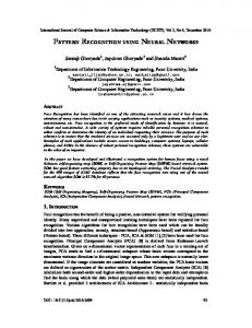
Transform pre-processing with the plane wave based fully probe corrected near-field transformation of low numerical complexity. The inherent nonlinearities associated with antenna radiation patterns make antennas very suitable candidates for ANNs. A major consequence that has emerged in recent years, with the growth of interest in NNs, is the Multilayer Perceptron (MLP) with single hidden layer. This network is capable of approximating any smooth nonlinear input-output mapping to an arbitrary degree of accuracy, provided that sufficient number of hidden layer neurons is used [10]. In [11] RBF neural network is used to optimize the radiation pattern of non-uniform linear arrays of High superconducting rectangular microstrip antennas. Phased array in communication system based on Taguchi-neural networks is presented in [12]. In [20] the authors present a usual application of back-propagation neural networks for synthesis and optimization of antenna array. In this paper, we are interest to present the adaptive Fourier Neural-Networks method that will be applied to the synthesis of antenna arrays. A big flexibility between features of the antennas array: amplitude and phase of feeding, ondulation domain, and secondary lobe level are introduced. For the simulation package we use the Matlab software and CST microwave studio. The paper is organized as follows. The synthesis problem formulation is presented in Section 2. Artificial Neural networks is developed with the simulation result in Section 3 and finally, Section 4 makes conclusions. 2. SYNTHESIS PROBLEM FORMULATION An antenna array is a configuration of individual radiating elements that are arranged in space and can produce direction radiation pattern. For a linear antenna array, let us assume that there are N isotropic radiators placed symmetrically along the x-axis as shown in Figure 1. The far-field F (u) of a linear array with N antennas arranged along a periodic grid at distance d apart, can be written as the product of the embedded element pattern EF (u) and the array factor AF (u) F (u) = EF (u)AF (u) (1) AF (u) =

N −1 ∑

wm ejkmdu

(2)

m=0

where • wm is the complex excitation of the mth element. ( ) • k is wave number 2π λ . • λ is the wavelength. • u = sin θ and θ angular coordinate measured between far-field direction and the array normal. z AF(ψ') = AF(ψ − ψo )

d Region I

(−M)

∆ψ stopband

(−1) 0

A

y

Region II

stopband attenuation

Region II

(+1)

ψ'

−π

(+M)

−ψ b

0

ψb

x

Figure 1. array.

Symmetrical placed linear antenna

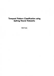
Figure 2. Desired radiation pattern.

π

Progress In Electromagnetics Research B, Vol. 67, 2016

47

2.1. Fourier Synthesis Method The array factor can be written with the DFT Discrete Fourier Transform or with z transformation as follows [22] : • If N is odd (N = 2M + 1). M ∑

AF (u) =

wm ejmψ = w0 +

(3)

m=1

m=−M

AF (z) ∼ = w0 +

M [ ] ∑ wm ejmψ + w−m e−jmψ

M ∑ [

wm z m + w−m z −m

]

(4)

m=1

where ψ = kdu and z = ejψ . In the following, we express array factor in a desired angular sector using the Fourier series method. For this we will present an ideal band pass filter centred ψo with the bandwidth of 2ψb , then this will plot actual characteristic as shown in Figure 2. Thus, the response of an ideal band pass filter is defined between −π ≤ ψ ≤ π as follows: { 1, ψ0 − ψb ≤ ψ ≤ ψ0 + ψb AFP B (ψ) = (5) 0, otherwise • If N is even (N = 2M ).

AF (u) = F (z) ∼ =

M ∑

M [ ] ∑ 1 1 wm ej (m− 2 )ψ + w−m e−j (m− 2 )ψ

1

wm ej (m− 2 )ψ =

m=1 M [ ∑

(6)

m=1

wm z (m− 2 ) + w−m z −(m− 2 ) 1

1

] (7)

m=1

In particular, if the array weights wm are symmetric with respect to the origin, wm = w−m , as they are in most design methods, then the array factor can be simplified into the cosine forms: AF (ψ) = w0 + 2

M ∑

wm cos [mψ],

m=1

F (ψ) = 2

M ∑

wm cos

m=1

[(

1 m− 2

N = 2M + 1

) ] ψ ,

N = 2M

(8)

(9)

In both for odd and even cases, the two Equations (4) and (7) can be expressed as the left-shifted version of a right-sided z-transform: AF (z) = z −(M −1) 2 AF˜ (z) ≈ z −(M −1) 2 1

1

M −1 ∑

w ˜m (z) z m

(10)

m=0

In the symmetric notation, the steered weights are as follows: ′ wm = wm e−jmψ0 , m = 0, ±1, ±2, . . . , M 1 w′ = w e±j (m− 2 )ψ0 , m =, 1, 2, . . . , M ±m

±m

(11) (12)

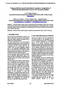
To justify the use of Fourier method, several well-known optimization methods; such as Taylor [23], Dolph-Chebyshev [24], Schelkunoff [25, 26] are selected for comparison. Best results obtained using Fourier. Best results are defined as the ones that provide a radiation pattern not only with SLL reduced but also with the best Half Power Beamwidth (HPBW) which is a very important pattern parameter for array synthesis. Figure 3 shows the radiation patterns of Taylor, Schelkunoff, Dolph-Chebyshev

48

Ghayoula et al.

as compared to Fourier method. The computational results from Figure 3 show that sidelobe level is reduced to −30 dB and more for all techniques but with HPBW about 4.5◦ for Taylor, 7◦ for Schelkunoff, 8◦ for Dolph-Chebyshev and about 18◦ with Fourier method. The obtained optimized array factor was compared to that obtained using other well-known numerical optimization techniques (Taylor, Schelkunoff and Dolph-Chebyshev). Array factor patterns synthesis obtained from Fourier results outperform the other methods. At the end of simulation, we have as a results different optimized values which are used as excitations for amplitude and phase. Our linear antenna array is optimized using Fourier method, so as expected, the ideal weights are used for the design of band pass filters ∆ θ = 70◦ , ∆ θ = 40◦ and ∆ θ = 5◦ . Ideal weights (amplitudes and phases) are summarized in Table 1. 0 Fourier Schelkunoff Taylor Dolph-Chebyshev

-10 -20

amplitude (dB)

-30 -40 -50 -60 -70 -80 -90 -100 0

20

40

60

80 100 θ (Deg)

120

140

160

180

Figure 3. Radiation pattern comparaison for a 16-antenna linear array.

Figure 4. Geometry of the proposed antenna.

Table 1. Fourier excitation linear array (at angle = 90◦ , M = 16 and d = 0.5λ). Fourier Excitation (M = 16 and d = 0.5λ ) θ1 = 50◦ and θ2 = 120◦ θ1 = 60◦ and θ2 = 100◦ θ1 = 75◦ and θ1 = 80◦ ◦ ◦ ∆ θ = 70 ∆ θ = 40 ∆ θ = 5◦ Number of elements m 1 2 3 4 5 6 7 8 9 10 11 12 13 14 15 16

Phase (deg.)

Amplitude

Phase (deg.)

Amplitude

Phase (deg.)

Amplitude

−83.61 83.53 −109.32 −122.17 44.97 −147.87 −160.72 6.42 −6.42 160.72 147.87 −44.97 122.17 109.32 −83.53 83.61

0.0029 0.0235 0.0290 0.0052 0.0674 0.0956 0.0068 0.5483 0.5483 0.0068 0.0956 0.0674 0.0052 0.0290 0.0235 0.0029

40.28 −169.08 161.54 −47.82 −77.19 −106.57 44.05 14.68 −14.68 −44.05 106.57 77.19 47.82 −161.54 169.08 −40.28

0.0137 0.0112 0.0350 0.0038 0.0742 0.0346 0.1777 0.4004 0.4004 0.1777 0.0346 0.0742 0.0038 0.0350 0.0112 0.0137

111.9154 −107.0067 −145.9287 175.1492 136.2272 97.3051 58.3831 19.4610 −19.4610 −58.3831 −97.3051 −136.2272 −175.1492 145.9287 107.0067 −111.9154

0.0046 0.0046 0.0216 0.0459 0.0747 0.1037 0.1277 0.1420 0.1420 0.1277 0.1037 0.0747 0.0459 0.0216 0.0046 0.0046

Progress In Electromagnetics Research B, Vol. 67, 2016

49

In this section a linear array structure of isotropic antennas with equal spacing of 0.5λ between any two consecutive elements has been considered. Minimization of sidelobe level is done using Fourier method. By controlling the phase and magnitude of the input signal assigned to each antenna element and the number of array elements, the radiation pattern can be steered in a desired direction with a preferred level of gain. In this example, a 16-array of patch antennas is fed from a single feed point, with all elements fed with synthesis phase and magnitude using Fourier method [5, 6, 21]. The synthesis results obtained with Fourier method of a 16 antennas are shown in Table 1. 2.2. Antenna Array Design The profile of the proposed antenna shown in Figure 4 is printed on a plexiglass substrate with relative permittivity of 2.5, loss tangent of 0.02, and thickness of 4 mm for IEEE 802.11 MIMO application [14]. The overall dimensions are L = 36 mm and W = 36 mm for 2.45 GHz. It was found that the antenna resonates in the desired frequency band as shown in Figure 5(a). Indeed, for |S11 | < −10 dB, we have band ranges from 1.5 to 3.5 GHz with a resonant frequency 2.45 GHz. The bandwidth is 105 MHz which is used for WLANs based on IEEE 802.11 applications. The desired sectors have variable width of the main beam of 70◦ , 40◦ and 5◦ . This is what can be seen in Figures 6(a), (b) and (c) an area with a main lobe (Region I) and another area with sidelobes (Region II) which has a level less than −30 dB below the level of the main lobe. Generally, with this method of synthesis, the desired radiation pattern requires an infinite number of coefficients that will be represented exactly. In addition only a fixed finite number of coefficients in the Fourier series has a corrugation in the desired response, known as Gibbs phenomenon [13]. S-Parameter Magnitude in dB 5 S1 1

0

S11 in dB

-5 -10 -15 -20 -25 -30 1.5

2

2.5

3

3.5

Fequency/GHz

(a)

(b)

Figure 5. Simulation results of the proposed patch antenna. (a) Reflection coefficient of the proposed antenna. (b) 3D Radiation pattern at 2.45 GHz.

3. ARTIFICIAL NEURAL NETWORKS The multi-layers networks consist of an input layer whose neurons code the information presented at the network, a variable number of internal layers called “hidden” and an output layer (Figure 7) containing as many neurons as the desired responses. The neurons of the same layer are not connected to each other. The learning process of these networks is supervised. The first layer is composed of input nodes. An MLP network is a feed forward neural network with one hidden layer, with a Multilayer Perceptron MLP node function at each hidden node. The number of nodes, L, is equal to the dimension of input vector [15–17]. • j is the index of the input layer with j = 1, 2, . . . , L.

50

Ghayoula et al.

(a)

(b)

(c) Figure 6. Radiation pattern for 16-antenna linear array with Fourier method. (a) ∆θ = 70◦ . (b) ∆θ = 40◦ . (c) ∆θ = 5◦ . ϕ(M) f2

ϕ(4)

4

M

ϕ(3)

ϕ(2)

ϕ(1)

2

3

yk

1 wki i = 1,...,N

f1

hi

5

N

4

3

2

1

wij j = 1,...,L

xj xL

x1

x2

x1

Figure 7. The neural beamformer architecture. • i is the index of the hidden layer with i = 1, 2, . . . , N . • k is the index of the output layer with k = 1, 2, . . . , M . The interconnection weights are determined based on the requirement of minimum error between

Progress In Electromagnetics Research B, Vol. 67, 2016

51

the neural model output yk and the training data dk . The purpose of the training process is to adjust the network interconnection weights wij and wki in order to minimize the error function E(p), defined by M N L 1 ∑∑∑ E (p) = [yk (xj , wij , wki ) − dk ]2 (13) 2 k=1 i=1 j=1

where p = 1, 2, . . . , P is the index of the training set. This is an iterative process using the backpropagation algorithm described in [12]. The weights wij and wki are updated for each iteration by ∂E (14) ∂wm The training-set examples included sector-width intervals of 10◦ , SLL intervals of −30 dB. The performance of the mean square error for MLP Network is shown in the above Figure 8. ∆wm = −η

Voltages (Phase)

Fourier Method

Radiation pattern

Neural network Error

Figure 8. Neural network training procedure. One of the major advantages of neural networks is their ability to generalize. This means that a trained network could classify data from the same class as the learning data that it has never seen before. In real world applications developers normally have only a small part of all possible patterns for the generation of a neural net. To reach the best generalization, the dataset should be split into three parts: • The training set is used to train a neural network: The error of this dataset is minimized during training. • The validation set is used to determine the performance of a neural network on patterns that are not trained during learning. • A test set for finally checking the overall performance of a neural network. We have two steps: I. Network designing 1. Form the input vectors {xp , p = 1, 2, . . . , 16}. 2. Generate input/output pairs {xp , φq }, where q = 1, 2, . . . , 18. 3. Design the Neural networks. II. Network testing (Generalization) 1. Form the vectors x′p for the testing input samples. 2. Present input vectors x′p to the neural networks. 3. Get the output of the network. The choice of the number of hidden neurons is strongly related to the nature of nonlinearity to model. In our case in Table 2, 30 hidden neurons allowed a good convergence of the algorithm and a good precision of the formed neuronal model. The neuron used in this network is the continuous nonlinear neuron whose function of activation is a tan sigmoid function (Table 3). To investigate the ideas presented in the previous section, the first step is dividing the space in to 18 sectors; repeat every 10 degrees in the interval from (5) degrees to (+175) degrees inclusively. More accurate space division sectors can be reached by increasing the number of element arrays. The input vector to the entry of neural network is in the form of a 18 bit binary code (one bit for each sector).

52

Ghayoula et al.

Table 2. Typical values of parameters use in Back-Propagation algorithm. Parameters

Symbol

Value

Neuron in the input layer

n

18

Neuron in the output layer

m

16

Neuron in the hidden layer

h

30

Coefficient of training

η

0.02

Table 3. Activation function. Parameters

Symbol

Function

The activation function at the hidden nodes

f1

Sigmoid tan

The activation function at the output nodes

f2

Sigmoid tan

Best Training Performance is 5.4053e-05 at epoch 10000

10

gradient

10 10

2

Gradient = 0.00071405, at epoch 10000

5

0

-5

Validation Checks = 0, at epoch 10000 1 10

10

0

val fail

Mean Squared Error (mse)

10

10

Train Best Goal

4

0

-2

-1 Learning Rate = 0.086848, at epoch 10000 1

-4

lr

10

10

0.5

-6

0

1000

2000

3000

4000

5000

6000

7000

8000

9000

0

10000

0

1000

2000

3000

10000 Epochs

4000

5000

6000

7000

8000

9000

10000

10000 Epochs

(a)

(b) Training: R=1 Data Fit Y=T

150

Output ~= 1*Target + -8.7e-06

100

50

0

-50

-100

-150

-150

-100

-50

0

50

100

150

Target

(c)

Figure 9. Neural networks results. (a) Performance. (b) Performance plot of the neural network training. (c) Training state of the network created during training.

Progress In Electromagnetics Research B, Vol. 67, 2016

53

A bin input of (+1) indicates a source exactly on (main lobe) in the sector. Convergence may then be achieved more rapidly. The proposed scheme (Figure 8) has been tested with excellent results, as shown in the following examples. A 16-element antenna array with centers separated is now used for synthesis purposes considering voltages with constant amplitude and variable phase [17–20]. The expected simulation results must show radiation patterns with sidelobe level SLL (at −30 dB), while maintaining main lobes in the direction of useful signal for the reference antenna (16 elements antennas array). In our application, the desired radiation pattern is specified at +10◦ to +170◦ , the database contains a whole of data(input/output) obtained by simulation with the Fourier method. Figures 9(a), (b) and (c) represents the training, validation, performance and testing data of the proposed neural networks structure. Figure 9(c) illustrates the graphical output provided by regression. The network outputs are plotted versus the targets as open circles. The best linear fit is indicated by a dashed line. The perfect fit (output equal to targets) is indicated by the solid line. In this application, it is difficult to distinguish between the best linear fit line and the perfect fit line, because the fit is so good. To illustrate the performance of the method described in the previous section for steering single beams in desired direction by controlling the phase excitation of each array element, 17 desired direction of uniform excited linear array with N = 16 half wavelength spaced isotropic elements were performed. Numerical results in Figure 10 show the excellent phase control capability for beam pattern synthesis by using Neural Networks with Fourier technique in different sectors. The synthesis excitation weights with neural networks are shown in Table 4 (part1) and Table 5 (part2). At the end of the neural network training phase, it is necessary to test it on a different data base from those used for learning. This test makes it possible both to assess the performance of the neural 0 @1 0

amplitude (dB)

-10

@2 0

-20

@3 0 @4 0

-30

@5 0 @6 0

-40

@7 0 @8 0

-50

@9 0

-60

@100 @110

-70

@120 @130

-80 -90

@140 @150 0

20

40

60

80

100

θ (Deg)

120

140

160

@160 180 @170

Figure 10. Radiation pattern of 16 elements λ/2 spaced array optimized using Fourier-Neural Network with respect to amplitudes (at −30 dB).

(a)

(b)

54

Ghayoula et al.

(c)

(d)

(e)

(f)

Figure 11. Cartesian representation of radiation pattern with 16 elements using Neural NetworkFourier method at 2.45 GHz. (a) At angle 60◦ . (b) At angle 70◦ . (c) At angle 80◦ . (d) At angle 90◦ . (e) At angle 100◦ . (b) At angle 110◦ .

Table 4. Neural network-Fourier excitation for linear array (M = 16 and d = 0.5λ) (part1). Neural network excitations (M = 16 and d = 0.5λ) Number of

Phase (deg.) ◦

◦

◦

◦

50◦

60◦

130.22

−35.53

07.13

−150.80

134.10

35.49

−86.06

elements m

10

20

30

40

1

−115.56

−176.24

−95.31

2

67.84

15.25

- 70.60

3

−108.75

−153.24

70◦

80◦

90◦

132.43

−80.02

53.53

−179.99

42.77

−141.35

22.39

−179.99

133.11

157.31

−08.74

−179.99

4

74.65

38.25

−21.18

−101.86

158.67

43.45

−84.01

140.11

0.00

5

−101.93

−130.24

−176.48

120.77

43.41

−46.19

−145.34

108.98

0.00

6

81.47

61.25

28.22

−16.59

−71.84

−135.85

153.32

77.84

0.00

7

−95.11

−107.24

−127.24

−153.95

172.89

134.48

91.99

46.70

0.00

8

88.29

84.25

77.64

68.68

57.63

44.82

30.66

15.56

0.00

9

−88.29

−84.25

−77.64

−68.68

−57.63

−44.82

−30.66

−15.56

0.00

10

95.11

107.24

127.24

153.95

−172.89

−134.48

−91.99

−46.70

0.00

11

−81.47

−61.25

−28.22

16.59

71.84

135.85

−153.32

−77.84

0.00

12

101.93

130.24

176.48

−120.77

−43.41

46.19

145.34

−108.98

0.00

13

−74.65

−38.25

21.18

101.86

−158.67

−43.45

84.01

−140.11

0.00

14

108.75

153.24

−134.10

−35.49

86.06

−133.11

−157.31

08.74

179.99

15

−67.84

−15.25

70.60

−07.13

150.80

−42.77

141.35

−22.39

179.99

16

115.56

176.24

95.31

−130.22

35.53

−132.43

80.02

−53.53

179.99

Progress In Electromagnetics Research B, Vol. 67, 2016

55

system and to detect the type of data that is problematic. If performance is not satisfactory, it will either change the network architecture or modify the learning base (discriminating characteristics or representativeness of each data class). In order to evaluate the proposed approach for the synthesis of linear arrays, many examples of simulations are investigated. The inter-element distances are d = 0.5λ. A simple patch antenna as shown in Figure 4 is employed and the working frequency of all the antenna arrays synthesised in this paper is 2.45 GHz. Using CST Microwave Studio (Figure 11), different simulation results with cartesian representation of radiation pattern for 16 antennas using Neural Network-Fourier method at 2.45 GHz (Figures 11(a), (b), (c), (d), (e) and (f)), it is clear that the criteria of −30 dB for sidelobe levels is fulfilled. Simulated results for 3D antenna radiation pattern synthesis of the developed MIMO antenna array system with 16 elements using Neural Network-Fourier method at 2.45 GHz are shown in Figure 12 and Figure 13. All these simulations are carried out using CST Microwave Studio simulator.

Table 5. Neural network-Fourier excitation for linear array (M = 16 and d = 0.5λ) (part2). Neural network excitations (M = 16 and d = 0.5λ) Number of

Phase (deg.) ◦

◦

120

130◦

140◦

150◦

160◦

170◦

−132.43

35.53

−130.22

95.31

176.24

115.56

141.35

−42.77

150.80

−07.13

70.60

−15.25

−67.84

−157.31

−133.11

86.06

−35.49

−134.10

153.24

108.75

−43.45

−158.67

101.86

21.18

−38.25

−74.65

145.34

46.19

−43.41

−120.77

176.48

130.24

101.93

−153.32

135.85

71.84

16.59

−28.22

−61.25

−81.47

−91.99

−134.48

−172.89

153.95

127.06

107.24

95.11

−15.56

−30.66

−44.82

−57.63

−68.68

−77.64

−84.25

−88.29

15.56

30.66

44.82

57.63

68.68

77.64

84.25

88.29

46.70

91.99

134.48

172.89

−153.95

−127.06

−107.24

−95.11

elements m

100

1

−53.53

2

−22.39

3

08.74

4

−140.11

84.01

5

−108.98

6

−77.84

7

−46.70

8 9 10

110

80.02

◦

11

77.84

153.32

−135.85

−71.84

−16.59

28.22

61.25

81.47

12

108.98

−145.34

−46.19

43.41

120.77

−176.48

−130.24

−101.93

13

140.11

−84.01

43.45

158.67

−101.86

−21.18

38.25

74.65

14

−08.74

157.31

133.11

−86.06

35.49

134.10

−153.24

−108.75

15

22.39

−141.35

42.77

−150.80

07.13

−70.60

15.25

67.84

16

53.53

−80.02

132.43

−35.53

130.22

−95.31

−176.24

−115.56

(a)

(b)

56

Ghayoula et al.

(c)

(d)

(e)

(f)

Figure 12. Simulated results for 3D antenna radiation pattern with 16 elements using Neural NetworkFourier method at 2.45 GHz (part1). (a) At angle 40◦ . (b) At angle 50◦ . (c) At angle 60◦ . (d) At angle 70◦ . (e) At angle 80◦ . (f) At angle 90◦ .

(a)

(b)

(c)

(d)

Progress In Electromagnetics Research B, Vol. 67, 2016

(e)

57

(f)

Figure 13. Simulated results for 3D antenna radiation pattern with 16 elements using Neural NetworkFourier method at 2.45 GHz (part2). (a) At angle 100◦ . (b) At angle 110◦ . (c) At angle 120◦ . (d) At angle 130◦ . (e) At angle 140◦ . (f) At angle 150◦ . In this paper, we use the non-linear neural representation to develop a new synthesis tool, and this radiation to meet the desired specifications. The validity of this model has been supported by various cases of simulation. Results clearly show a very good agreement between the desired and synthesized specifications. 4. CONCLUSION In this paper, a hybrid synthesis method is proposed to design linear antenna array for the given optimal radiation pattern using Neural Networks. To have a good optimization results in linear arrays, the parameters that should be controlled are the excitations of antennas. This paper deals about finding the parameters of radiation pattern of given uniform linear antenna array. Initially, the network is trained with a set of input-output data pairs based on Fourier synthesis phases. We studied the possibilities of modeling and optimization of the synthesis problem for the antenna arrays with the Fourier method and neuronal approach. Results show that there is an agreement between the desired specifications and the synthesized one. This demonstrates the effectiveness of the proposed procedure. The Neural-Networks have better learning ability, generalization, parallel processing and error endurance attributes that lead to perfect solutions in applications where one needs to model the nonlinear mapping of complex data. This approach makes use of Neural Network that can be trained for any number of elements, spacing and excitation. Once the network is trained, it can find the parameters with respect to the input. REFERENCES 1. Yan, K. K. and Y. Lu, “Sidelobe reduction in array-pattern synthesis using genetic algorithm,” IEEE Transactions on Antennas and Propagation, Vol. 45, No. 7, 1117–1122, July 2007. 2. Khodier, M. M. and C. G. Christodoulou, “Linear array geometry synthesis with minimum sidelobe level and null control using particle swarm optimization,” IEEE Transactions on Antennas and Propagation, Vol. 53, No. 8, 2674–2679, August 2005. 3. Recioui, A., “Sidelobe level reduction in linear array pattern synthesis using particle swarm optimization,” Jour. of Optimization Theory and Applic., Vol. 153, 497–512, 2012. 4. Zhang, L., Y. C. Jiao, Z. B. Weng, and F. -S. Zhang, “Design of planar thinned arrays using a Boolean differential evolution algorithm,” Microwaves Antennas and Propagation IET , Vol. 4, No. 12, 2172–2178, December 2010. 5. Keizer, W. P. M. N., “Fast low sidelobe synthesis for large planar array antennas utilizing successive fast fourier transforms of the array factor,” IEEE Transactions on Antennas and Propagation, Vol. 56, No. 8, 715–722, March 2007.

58

Ghayoula et al.

6. Keizer, W. P. M. N., “Linear array thinning using iterative fourier techniques,” IEEE Transactions on Antennas and Propagation, Vol. 55, No. 3, 2211–2218, August 2008. 7. Trastoy, A. and F. Ares, “Phase-only control of antenna sum patterns,” Progress In Electromagnetics Research, Vol. 30, 47–57, 2001. 8. Lee, K. C. and J. Y. Jhang, “Application of electromagnetism-like algorithm to phase-only syntheses of antenna arrays,” Progress In Electromagnetics Research, Vol. 83, 279–291, 2008. 9. Carsten, H. S., T. F. Eibert, and T. A. Laitinen, “Hybrid fast fourier transform-plane wave based near-field far-field transformation for body of revolution, antenna measurement grids: The cylindrical case,” IEEE International Symposium on Antennas and Propagation (APSURSI), 1628– 1631, Spokane, WA, 2011. 10. Sarevska, M., “Signal detection for neural network-based antenna array,” Conf. NAUN’08 on Circuits, Systems, and Signals, 115–119, Marathon, Attica, Greece, June 2008. 11. Barkat, O. and A. Benghalia, “Optimization of superconducting antenna arrays using RBF neural network,” Int. J. Simul. Multidisci. Des. Optim., Vol. 4, 2010. 12. Smida, A., R. Ghayoula, H. Trabelsi, A. Gharsallah, and D. Grenier, “Phased arrays in communication system based on taguchi-neural networks,” Wiley International Journal of Communication Systems, John Wiley and Sons, September 2013. 13. CST Microwave Studio, “CST microwave studio 2013 by computer simulation technology,” http://www.cst.com, 2013. 14. Chang, D.-C., Y.-J. Li, and C.-H. Liao, “Antenna array for IEEE 802.11/a/b MIMO application,” PIERS Proceedings, 100–102, Moscow, Russia, August 19–23, 2012. 15. Kunis, S. and D. Potts, “Time and memory requirements of the nonequispaced FFT,” Sampling Theory in Signal and Image Processing, Vol. 7, 77–100, 2008. 16. Castaldi, G., V. Galdi, and G. Gerini, “Evaluation of a neural-network-based adaptive beamforming scheme with magnitude-only constraints,” Progress In Electromagnetics Research B , Vol. 11, 1–14, 2009. 17. Gotsis, K. A., K. Siakavara, and J. N. Sahalos, “On the direction of arrival (DoA) estimation for a switched-beam antenna system using neural networks,” IEEE Transactions on Antennas and Propagation, Vol. 57, No. 5, 1399–1411, May 2009. 18. Vakula, D. and N. V. S. N. Sarma, “Using neural networks for fault detection in planar antenna arrays,” Progress In Electromagnetics Research Letters, Vol. 14, 21–30, 2010. 19. Reza, S. and C. G. Christodoulou, “Beam shaping with antennas arrays using neural netsworks,” IEEE SouthEast Conf., Orlando, Florida, April 1998. 20. Merad, L., F. T. Bendimerad, S. M. Meriah, and S. A. Djennas, “Neural networks for synthesis and optimization of antenna arrays,” Radioengineering, Vol. 16, No. 1, April 2007. 21. Keizer, W. P. M. N., “Low-sidelobe pattern synthesis using iterative fourier techniques coded in MATLAB,” IEEE Transactions on Antennas and Propagation, Vol. 51, No. 2, 137–150, April 2009. 22. Sophocles, J. O., “Electromagnetic waves and antennas,” Vol. 21, Rutgers University, June 2004. 23. Abed, A. T., “Study of radiation properties in Taylor distribution uniform spaced backfire antenna arrays,” American Journal of Electromagnetics and Applications, Vol. 2, No. 3, 23–26, May 2014. 24. Fadlallah, N., L. Gargouri, A. Hammami, R. Ghayoula, A. Gharsallah, and B. Granado, “Antenna array synthesis with Dolph-Chebyshev method,” 11th Mediterranean Microwave Symposium (MMS 2011), Yasmine Hammamet, Tunisia, September 8–10, 2011. 25. Marcano, D., M. Jiminez, and O. Chang, “Synthesis of linear array using Schelkunoff’s method and genetic algorithms,” Antennas and Propagation Society International Symposium, 1996. AP-S. Digest, Vol. 2, No. 3, 814–817, Baltimore, MD, USA, July 21, 1996. 26. Marcano, D. and F. TDuran, “Synthesis of antenna arrays using genetic algorithms,” IEEE Antennas and Propagation Magazine, Vol. 42, No. 3, 12–20, August 06, 2002.