Perceiving patterns in parallel coordinates: determining thresholds for identification of relationships ∗
Jimmy Johansson∗,1 , Camilla Forsell∗ , Mats Lind† , and Matthew Cooper∗ Norrk¨oping Visualization and Interaction Studio, Link¨oping University, Sweden † Department of Information Science, Uppsala University, Sweden
Abstract This article presents a study that investigates the ability of humans to perceive relationships (patterns) in parallel coordinates, an ability that is crucial to the use of this popular visualization technique. It introduces a visual quality metric, acceptable distortions of patterns, which establishes the level of noise that may be present in data while allowing accurate identification of patterns. This metric was used to assess perceptual performance of standard 2D parallel coordinates and multi-relational 3D parallel coordinates in two experiments. In multi-relational 3D parallel coordinates the axes are placed on a circle with a focus axis in the centre, allowing a simultaneous analysis between the focus variable and all other variables. The experiments aimed to determine the maximum number of variables that can be, from a user’s point of view, efficiently used in a multi-relational 3D parallel coordinates display and to present a first attempt to study users’ ability to analyse noisy data in parallel coordinates. The results show that, in terms of the acceptable level of noise in data, a multi-relational 3D parallel coordinates visualization having 11 axes (variables) is as efficient as standard 2D parallel coordinates. Visualizing a larger number of variables would possibly require a greater amount of manipulation of the visualization and thus be less efficient.
1
Introduction
Within many domains decision making requires extensive exploration and analysis of data. To facilitate these processes information visualization techniques are offered for use. New methods and tools emerge all the time but not all of these techniques are equally suited to all situations. The critical question is how to create visualization techniques that can be effectively and efficiently applied by users in order to discover the relevant structures contained in the data. A commonly used information visualization technique is parallel coordinates [1, 2] which is used for visualizing multivariate data. In parallel coordinates the axes are placed parallel and equally separated. Each axis corresponds to a variable and each data item, having values for all variables, is represented as a series of line segments intersecting the axes at the corresponding values, see figure 1. With this axis configuration only relationships between variables mapped to adjacent axes can be directly analysed. One extension of standard 2D parallel coordinates is multi-relational 3D parallel coordinates [3]. Here the axes are placed, equally separated, on a circle with a focus axis in the centre. A data item is again displayed as a series of line segments intersecting all axes, see figure 1. This axis configuration has the advantage that all pairwise relationships between the focus variable in the centre and all outer variables can be investigated simultaneously. 1
[email protected]
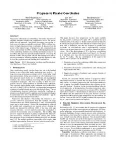
Figure 1: Illustrations of standard 2D parallel coordinates (left) and multi-relational 3D parallel coordinates (right). In standard parallel coordinates it is only possible to examine the relationship between variables mapped to adjacent axes. In multi-relational 3D parallel coordinates a simultaneous analysis between a focus variable (A) and all other variables is possible.
The standard 2D parallel coordinates technique has previously been compared with multi-relational 3D parallel coordinates with the objective to identify classes of user tasks for which each representation is best suited [4]. The 3D layout was shown to be superior to the 2D layout in revealing relationships (patterns) in a multivariate data set. It has an obvious advantage for this task in that the configuration enables a simultaneous analysis of the relationships between the focus axis and all other axes, but this comes at the cost of having the relationships distorted by perspective effects [5]. This is, however, of no hindrance as long as the patterns have properties that are invariant under affine transformations. These properties are qualitative in nature and based on structures that are easily picked up by the visual system regardless of the perspective [6, 7]. This work extends the investigation of the usability of multi-relational 3D parallel coordinates. In particular it investigates how many variables in a data set can, from a users’ point of view, be meaningfully shown in one view of the visualization. The work also presents a first effort to investigate the ability of the users to analyse noisy data, perceiving patterns subject to noise. This is an important visual quality metric to be considered when assessing the usability of a visualization since a visualization of a real, large multivariate data set is likely to contain noise that distorts the patterns. These issues are addressed in two steps. The first experiment investigates the threshold of acceptable noise present in data for a frontoparallel viewing condition which represents the use of a standard 2D parallel coordinates visualization. The second experiment tests whether different angles between the outer axes (corresponding to visualizing different numbers of variables) in multi-relational 3D parallel coordinates have any effect on the threshold, as compared to standard 2D parallel coordinates. Finding if there is a breaking point at which the noise threshold significantly decreases, will help in determining the limit on the number of variables that can be used in multi-relational 3D parallel coordinates. In summary, the major contributions of this article are: • the introduction of a visual quality metric, acceptable distortions of patterns, to be used as a measurement tool in evaluation • the determination of an upper limit of noise for which a pattern can be recognized in standard 2D parallel coordinates
• the determination of how the angle of viewing in multi-relational 3D parallel coordinates affects the acceptable noise level • the establishment of an upper limit on the number of variables that can be meaningfully displayed in multi-relational 3D parallel coordinates The remainder of this article is structured as follows. The next section presents and discusses recent related work on 2D and 3D extensions of parallel coordinates relevant to the research issues of this article. The following section describes the general experimental method used in this study and the visual quality metric used to measure performance. The next two sections describe the two experiments performed. The final sections discuss the general results and outline some issues for future research.
2
Background and related work
The parallel coordinates technique [1] is extensively used within a wide range of domains and has many applications. Some recent examples include using parallel coordinates for analysing multichannel EEG data [8], as a user interface to facilitate exploration of volume data [9] and as an integrated tool in a larger system for analysing spatio-temporal and multivariate patterns [10]. To increase its applicability, standard 2D parallel coordinates has been subject to many extensions which can broadly be categorized into two main areas: clutter reduction approaches and axis configuration approaches. The parallel coordinates technique is not well suited to visualization of large data sets. The limit on how many data items can be displayed simultaneously varies from application to application but is usually in the range of hundreds. Visualizing a larger data set will inevitably result in a cluttered image which impairs the analysis process. Reducing clutter in parallel coordinates has, therefore, attracted the attention of many researchers and several interesting approaches have been proposed [11, 12, 13, 14, 15]. Another aspect that affects the visual result is the order in which axes are positioned. In standard 2D parallel coordinates it is only possible to analyse the relationships between variables mapped to adjacent axes and to completely investigate all relationships within a multivariate data set using such a visualization requires substantial interaction and memorization between different views. For standard 2D parallel coordinates this can primarily be addressed in two ways: using an algorithm to calculate all permutations needed in order to visualize all possible pairwise combinations [2], or ordering axes according to certain features in the data, for example by minimizing outliers [16]. By changing the standard 2D parallel axis layout to a circular 2D arrangement [17], a simultaneous analysis between a single focus variable and all other variables is made possible. However, in this axis configuration the outer variables are not all parallel to the focus axis. This limits the analysis process since it may be difficult to interpret the appearance of patterns. A 3D version of this approach that deals with this limitation was proposed by Johansson et al. [3]. In this multi-relational 3D configuration all axes are parallel. The technique has been found [4] to significantly decrease the time required to find relationships within multivariate data sets compared with standard 2D parallel coordinates. Another example of extending 2D parallel coordinates into 3D uses planes, instead of lines, as axes [18, 19]. This approach does not directly deal with the issue of how to order axes but, since an extra spatial dimension is added, more variables can be displayed simultaneously. This advantage is weakened, however, by the fact that 3D visualizations often suffer from perspective distortions, making comparison of individual data items at different positions in depth difficult and distorting the perception of patterns in data. The advantages of the multi-relational 3D parallel coordinates technique, as compared with the other 2D and 3D extensions discussed above, are primarily: (1) that it reduces visual complexity, interaction and mental effort required to fully analyse all possible pairwise relationships within a multivariate data set, and (2) that each pairwise relationship under analysis is rendered between two parallel axes and so all lines are coplanar, no comparison between lines within planes at different depths is required.
Figure 2: The five stimulus patterns used in the study. From left to right: negative linear relationship, negative linear relationship with a discontinuity, sinusoidal relationships with one, two and three periods respectively.
Despite these advantages, when using a 3D layout for data representation the possibility of misleading distortions caused by the perspective view has to be taken into consideration. Current theory and empirical findings [20, 21, 22] claims that the suitability of 3D visualizations is restricted to qualitative judgements since only a class of qualitative properties of structure in 3D space are easily perceived, namely those invariant under affine transformations. Metric judgements, however, are ambiguous and such properties are not accurately perceived. Hence, 3D visualization is well suited to aid user tasks that require the determination of the nature of relationships between variables rather than the strength of relationship (for example, the correlation). This has been successfully shown by Forsell and Johansson [4] and the work presented in this article continues to focus on parallel coordinates as an aid for users in determining the nature of relationships in data.
3
General experimental method
This section describes the general method used in the study and outlines some of the issues in experimental theory motivating the operational definitions used. The specific experiments are explained in more detail in the subsequent sections describing experiments 1 and 2.
3.1
Task
To evaluate the ability to perceive patterns subject to noise a judgement situation to be performed as a discrimination task was created. The participants were asked, in any individual experimental trial, to identify a stimulus pattern displayed for a certain duration. In this context, a pattern means a relationship in data created between a single pair of axes in a parallel coordinates visualization.
3.2
Patterns
Evaluating performance of the perceptual issues considered in this study requires clearly defined answers, thus the data set employed must contain a well-defined set of patterns that the participants can identify without interference from other factors [23]. In order to have full control of the patterns present in the study five mathematical relationships were used (the test data set and the mathematical relationships were constructed in an earlier work and are described in detail by Forsell and Johansson [4]). The five stimulus patterns depicted the following mathematical relationships: a negative linear relationship, a negative linear relationship with a discontinuity, and sinusoidal relationships with one, two and three periods (see figure 2). The participants in the study were not required to learn anything about the identity and nature of the variables or the relationships. They only had to recognize and discriminate between the patterns. All patterns were formed by the totality of 300 lines between two adjacent axes in the parallel coordinates display. The lines were rendered using transparency in order to make overlaps
Figure 3: A negative linear relationship formed between two variables mapped to adjacent axes in parallel coordinates. Each image shows the relationship with different amounts of added Gaussian noise. From left to right the pattern is displayed with: 0.0, 3.0, and 6.0 percent noise added to both variables.
more visible. This is a common technique which is extensively used today and was first explored together with parallel coordinates by Wegman and Luo [12]. Depending on how two axes were positioned with respect to each other, a stimulus pattern could be mirrored. These two different patterns (the stimulus pattern and its mirror reflection) were to be regarded as one and the same pattern. They differ only in orientation.
3.3
Noise
In each experimental trial one single pattern, subject to a certain level of noise, was presented. This means that the pattern was distorted when compared with its standard reference (zero noise as in figure 2). For some level of noise identification based on qualitative (affine) properties is no longer possible and that point represents the threshold noise value. The distortions in the patterns were introduced by adding Gaussian noise with mean value zero and varying standard deviation, σ, to both variables creating the pattern. The level of noise was defined as the ratio between σ and the range of the variables, hereinafter referred to as the percentage of noise. For example, adding Gaussian noise with σ = 0.01 to a variable having values between −0.5 and 0.5 gives one percent noise. Figure 3 illustrates a linear negative relationship subject to different levels of noise.
3.4
Pattern groups
The patterns were divided into two groups having three patterns each (one pattern belonged to both groups) that were tested in two separate experimental sessions, see figure 4. The main purpose for the grouping was to make the task less complicated for the participants in not having all five patterns as response alternatives at once. But, it also provides an opportunity to statistically test if there were any effects of the different patterns, that is, if one group of patterns were more easy or difficult to identify with respect to the amount of distortion (however the study did not aim to explicitly measure any differences between the individual patterns). In accordance with the grouping, each experiment followed the three alternatives forced choice (3 AFC) paradigm [24]. Consequently, the participants’ task was always to select one out of three possible response patterns, that is to discriminate between and decide which of the three possible stimulus patterns was presented. As an aid for the identification task the participants had instructional materials where the three standard reference patterns, for the specific group examined, were illustrated. The patterns were labelled from 1–3 and these numbers were used to record the response.
3.5
Adaptive procedure
To reach a threshold estimation of performance an adaptive staircase-procedure was used [25, 26, 27]. In this psychophysical method an observer’s ability to identify a stimulus is manipulated by varying the
Figure 4: Illustrations of the two pattern-groups used. Pattern-group A consists of a negative linear relationship, a negative linear relationship with a discontinuity and a sinusoidal relationship with one period (left). Pattern-group B consists of sinusoidal relationships with one, two and three periods (right).
intensity of the stimulus (here the level of noise) over a number of tasks (the staircase). The objective is to find the intensity level that corresponds to a prescribed response probability. This percentage point of certainty estimates the intensity level on the basis of the rule used to move up or down the staircase [27]. In the present study, the following rule was used: if the participant chose the wrong pattern once, the following task was made easier by decreasing the amount of noise (a down sequence); if the participant responded accurately two times in a row, the task was made more difficult by increasing the amount of noise on the subsequent task (an up sequence). The staircase converges on the stimulus level at which the probability of an up sequence equals the probability of a down sequence, that is a probability of 0.5. For the chosen two-up one-down staircase method a positive response (+) followed by another positive response give an up sequence (++). A positive response followed by a negative response (−) or a single negative response gave a down sequence (+− or −). The probability of an up sequence is therefore 2 (P (x)) , where P (x) is the probability of a positive response at stimulus level x, and the probability 2 of a down sequence is P (x) (1 − P (x)) + (1 − P (x)). Setting (P (x)) = 0.5 gives P (x) = 0.707 which means that the two-up one-down staircase procedure will converge on that level of noise at which the participants can correctly identify the patterns with a certainty of 70.7 percent. This decision rule was applied in combination with the 3AFC response procedure, described above, which is recommended since forced-choice procedures with more than two alternatives provide more satisfactory measurements of psychometric performance [28]. For further details on this procedure, and the specific operational definitions described here and in the detailed methods section below, the interested reader is referred to, for example, Cornsweet [25], Leek [26] and Levitt [27].
3.6
Usability criterion — evaluating the efficiency of visualizations
When evaluating a visualization by means of a user study the aim is to measure a possible effect of the visualization. What to measure against is an important question that can be approach by using the concepts of effectiveness and efficiency as defined in the ISO-standard 9241-11 [29]. The effectiveness of a visualization refers to the extent to which a task or goal is achieved, regardless of the effort spent. Efficiency is determined by the cost to solve the task and is most often measured in terms of the time needed to extract the relevant information contained in the visualization. This will largely be determined by the number of repeated fixations a viewer needs in order to accomplish the task. Hence, concerning the evaluation of visualizations this is a very important metric to consider. Such an approach was used by Lightner [30] who used the following model to calculate the minimum time, Tmin , in milliseconds (ms) needed for a viewer to accurately investigate a visualization: Tmin = 200 + 230(A − 1) where A is the number of areas (for example an object or parts of an object) that has to be fixated upon in a visualization to solve the task (where no re-fixations take place). The rationale behind the model is that a fixation usually lasts for around 200 ms and that an average saccade (movement of the eye) takes
about 30 ms. Since these figures are, of course, only approximations [31] the model can therefore be further simplified into Tmin = A/4, Tmin now measured in seconds [32]. Despite these approximations this estimate can be a useful guide to user performance efficiency [32, 33]. An important theoretical issue to consider when applying the model is that high-accuracy vision is restricted to a small foveal region surrounding the current fixation. This focal point has a fine grain resolution over only about two degrees of visual angle [34] with acuity dropping off rapidly away from the fovea. Consequently, the amount of high-quality information in a visualization that can be encoded in one glance is limited. Hence a judgement situation that, theoretically, has a stimulus exposure duration restricted to one fixation per part of a stimulus will give an estimate of the ability to efficiently decode (perceive) the important structural information in a visualization indicating that no re-fixations are necessary. This usability criterion of efficiency is taken into consideration when deciding on stimulus presentation in the two experiments that will be described in detail below.
4
Experiment 1
The purpose of experiment 1 was to begin an investigation of acceptable distortions in data. This perceptual ability was tested with patterns judged from a frontoparallel viewing position which corresponds to using a standard 2D parallel coordinates visualization. The result from this 2D viewing condition will also serve as a reference value when interpreting the performance of different 3D views of the patterns in experiment 2.
4.1
Method
This section describes the remaining details regarding the method chosen and the design of the experiment (not covered in the general method section). 4.1.1
Stimuli
The stimulus patterns (figure 2) in the present study were square shaped with a side of 3.6 cm and so having an area of 12.96 cm 2 . They were presented on a display placed at a standard viewing distance of approximately 57.0 cm so that 1.0 cm of the screen corresponded to 1.0 degree of visual angle. The square area can thus be divided into four subparts of 1.8 × 1.8 cm each. Considering the theoretical concerns given above, a reasonable approximation is that a subpart of a pattern can be identified with certainty within an angle in the visual field having a diameter of roughly 2 cm. This experimental setup means that the number of fixations needed by an observer to successfully investigate a stimulus pattern, where no re-fixations are necessary, can be predicted to be around 4. Hence the minimum expected time to solve the task, and an efficient measure of performance, indicating that no re-fixations are necessary in order to identify a pattern would be 1.0 second (4 fixations, each 250 ms per 1.8 × 1.8 subpart). 4.1.2
Apparatus and viewing setup
The experiment was carried out on a PC running Microsoft Windows with an Nvidia GeForce 4 graphics card. The stimulus patterns were shown on a 17” TFT monitor set at a resolution of 1280 × 1024 pixels. The patterns were produced through a program that showed each pattern against a white background. Each participant was seated in front of the monitor. The viewing position was unrestricted, however, the chair was adjustable and the participants were assisted to adjust their viewing position such that their eyes were centred at the screen. The participants interacted with the program by means of a keyboard.
4.1.3
Experimental design
The study was designed as a two factor, mixed factorial design with group of target pattern (patterngroup A and B) as within-subject factor and the order of presentation of the two groups as betweensubject factor. Half of the participants started with the three patterns that belonged to pattern-group A and the other half of the participants started with the three patterns that belonged to pattern-group B. The participants were randomly assigned to this sequence of tasks. The two-up one-down staircase method, together with the 3AFC response procedure described earlier, was used to obtain the two threshold estimates, one for each pattern-group. Each staircase was covered by 75 trials and the three patterns included appeared 25 times each in a randomized order of presentation. This design yielded a total of 150 trials per participant (75 trials×2 pattern-groups). Some preliminary runs with the authors and naive participants led to an expectation of a threshold value in the vicinity of 10 percent noise. This value was used as the start value in the staircase. In accordance with the up-down method chosen, a negative response decreased the noise level by one step and two correct responses increased it by one step. Distortion (one step) was introduced in units of 1.0 percent noise. 4.1.4
Procedure
Before the start of the experiment the participants reviewed written instruction material. The administrator explained the task, demonstrated the apparatus and then the experiment commenced. The experiment consisted of two sessions, one for each pattern-group. Each session, in turn, was divided into two parts: an introduction and training session for familiarizing the participant with the task and the experimental trials part. The participants were shown printed images representing the three patterns included in the task. They were extensively instructed about the specifics of each standard reference pattern and how distortions affect their appearance in order to understand the concept. They also completed a block of practice trials. The administrator helped participants when needed during the training session to resolve any confusion about how to operate the software and carry out the task before the experimental trials part began. The participants’ task in any individual trial was to respond to which of the three possible standard reference patterns was the target pattern of each trial. The sequence of trials was self-paced and the participants controlled the screen by pressing the space bar when they wished a trial to begin. Each trial comprised a sequence of images. A fixation cross was first presented at the centre of the screen. When the participant pressed the space bar a pattern was presented for a duration of 1.0 second followed by a blank screen. The blank screen was displayed until a response was given. This completed a trial and the fixation cross reappeared and the experiment continued. The response keys used were the numbers 1–3 on the numerical keyboard. Each number corresponded to one of the three possible standard reference patterns. These were depicted (without noise) and enumerated on instructional materials. Responses and noise level were recorded for each trial. No feedback was provided. Total participation time in the experiment was approximately 20 minutes (including the introductory parts). 4.1.5
Participants
Twelve participants took part in the experiment, seven men and five women. They were all students or staff at Link¨ oping University, campus Norrk¨oping, aged between 23 and 42 years. The participants had no prior knowledge of the purpose of the experiment. All of the participants declared that they had normal or corrected to normal vision. They received a small compensation for taking part in the experiment.
Figure 5: The five relationships used as stimulus patterns are illustrated with a noise level of 13 percent. From left to right: negative linear relationship, negative linear relationship with a discontinuity, sinusoidal relationships with one, two and three periods respectively. As a comparison, below each stimulus pattern, the corresponding scatter plot is shown. The signal-to-noise ratios of the variables are also presented in table 1.
Negative linear relationship Negative linear relationship with a discontinuity Sinusoidal relationship with one period Sinusoidal relationship with two periods Sinusoidal relationship with three periods
Variable 1 (ratio) 4.3:1 4.3:1 4.3:1 4.3:1 4.3:1
Variable 2 (ratio) 4.3:1 5.6:1 6.4:1 6.4:1 6.4:1
Table 1: Signal-to-noise ratios of the variables that give rise to the five patterns used in the experiment for a noise level (as defined above) of 13 percent. The five patterns are visualized in figure 5.
4.2
Results
Data from all 12 participants were analysed. For each of them the mean threshold value was calculated from the noise levels of the final four reversal points on the 75 trial staircase for each pattern-group. A reversal means that there is a change in direction of stimulus change, from an up sequence to a down sequence, or vice versa. This calculated mean threshold value was used as the dependent measure. A mixed ANOVA was carried out using a decision criterion of 0.05. Within-subject factor was group of patterns (group A and group B). Between-subject factor was order of presentation of pattern-group (AB and BA). There was no significant effect of pattern-group (F (1, 10) = 3.263, p = 0.11) and no significant effect of the ordering factor (F (1, 10) = 1.675, p = 0.225). Since no effect of pattern-group was obtained each participant’s data was collapsed over the two pattern–groups. The global mean value of the noise was 13.01 percent with a standard deviation of 2.73.
4.3
Discussion
The aim of this experiment was to investigate users’ perceptual ability to recognize different relationships in data when these were visualized with added noise. At a certain level of noise identification is no
α
α
β
Figure 6: Illustrations of rotations of stimulus patterns in multi-relational 3D parallel coordinates seen from above (left) and seen from the front (right). Three different angles of α were used; 30, 18 and 10 degrees corresponding to 7, 11 and 19 variables. β was fixed to 45 degrees to simulate the appearance of the multi-relational 3D parallel coordinates visualization.
longer possible and the objective was to find this threshold value. The result suggests that for the given reliability of 70.7 percent, this computed threshold value for an acceptable noise level is around 13 percent. See figure 5 for an illustration of the five patterns with 13 percent noise added. Also, as a comparison with the visual representations, the signal-to-noise ratios (SNRs) of the corresponding five pairwise variables are presented in table 1. One variable is included in all relationships and has an SNR of 4.3:1. For pattern-group A the SNRs of the second variable in the relationships has ratios between 4.3:1–6.4:1. For pattern-group B all SNRs are the same. Despite the difference in SNRs between the pattern groups no significant difference in threshold value was found between the groups. Since our experiment is based on the percentage of noise in the data, and since the SNR in the pattern groups does not show any significant differences this will not be discussed any further.
5
Experiment 2
Using the same basic paradigm as in the first experiment, this second experiment was aimed at finding the noise threshold values for different perspective views in multi-relational 3D parallel coordinates. The goal was to examine whether differences in viewing angle (α in figure 6), caused by different numbers of axes, would translate into actual performance differences in perceiving noisy patterns. An answer to this question will help in determining the upper limit on the number of axes, and so the number of variables contained in a data set, that can be meaningfully shown in a single rendering of the visualization. Three different viewing angles, equivalent to three possible numbers of axes, were measured and compared. The patterns were also rotated (β = 45 degrees) around a horizontal axis to simulate the actual appearance in 3D multi-relational parallel coordinates. This angle was chosen since most users that have interacted with the visualization and experienced the ability to freely rotate it, not only viewed its appearance as in the present study, have rotated it to between 30 and 60 degrees.
Figure 7: Multi-relational 3D parallel coordinates visualizing a data set consisting of 7 (left), 11 (middle) and 19 (right) variables.
5.1
Method
This section describes the remaining details regarding the method chosen and the design of the experiment (not covered in the general method section). 5.1.1
Stimuli
The five patterns and the two pattern groups from experiment 1 were used. The patterns were visualized at three different viewing angles (α in figure 6): 30, 18 and 10 degrees. These angles in turn represent the worst case viewing scenario, that is the smallest viewing angles in visualizations having 7, 11 and 19 variables respectively (figure 7). A viewing angle of 30 degrees creates a visualization having a total of 7 variables. One variable is placed as the focus variable and the 6 outer variables are placed, equally spaced with an angle of 2α = 60 degrees. Similarly a viewing angle of 18 degrees creates a visualization having a total of 11 variables and a viewing angle of 10 degrees creates a visualization having a total of 19 variables. Only two axes were shown for each trial (the focus axis and one of the outer axes), rather than the complete set of axes (7, 11 or 19). Regarding the size of the stimulus patterns, for the 30 degree condition it was the same as in experiment 1, that is 12.96 cm 2 . For the other two conditions, 10 and 18 degrees, the decreasing angle obviously results in slightly smaller areas for the stimulus patterns. Regardless of these minor differences the same prediction in terms of search time for efficient performance was made to create a comparability between all conditions. The presentation time for each stimulus was again 1.0 second. All viewing conditions, including the 2D view from experiment 1, are illustrated in figure 8. 5.1.2
Apparatus and viewing setup
The same type of apparatus, computer program and viewing setup as in experiment 1 was used. 5.1.3
Experimental Design
This study was designed as a three factor mixed factorial design with two within-subject factors: viewing angle (10, 18 and 30 degrees) and group of target patterns (group A and group B). The between-subject factor was the order of presentation of the two groups (AB and BA). Every second participant started with the patterns that belonged to group A, the rest started with the patterns that belonged to group B. The participants were randomly assigned to this sequence of tasks. The two-up one-down staircase used in experiment 1 was used to obtain the six threshold estimates, one for each of the three different angles of 10, 18 and 30 degrees within each pattern-group. Each angle constituted one condition and
Figure 8: An illustration of the different viewing conditions used in both experiments. From left to right: an angle (α) of 90 degrees corresponds to the 2D display used in experiment 1, and angles of 30, 18 and 10 degrees were used in experiment 2. These correspond to 7, 11 and 19 variables in multi-relational 3D parallel coordinates (figure 7). Here the patterns were also rotated with β = 45 degrees to simulate their actual appearance in multi-relational 3D parallel coordinates.
each condition was covered by a staircase with 50 trials. Within each experimental session (patterngroup), the three separate staircases were run concurrently and picked randomly on each trial. The number of trials for each staircase was less than in experiment 1. The rationale behind this was economy in mental effort and time and the difference should not have any effect on the assessment of a fairly reliable threshold-value. For each of the conditions an equal number of patterns were presented and they appeared in a randomized order of presentation. Thus each trial presented a stimulus consisting of either pattern 1, 2 or 3 presented by a viewing angle of 10, 18 or 30 degrees. Interleaving several independent staircases reduces the predictability of the stimulus presentation in the next trial [27]. Also, assessing the three thresholds simultaneously, rather than sequentially avoids the possibility of practice biasing the result. Finally effects of fatigue or boredom are also removed. To summarize, each participant judged a total of 300 stimuli (50 trials×3 angles×2 pattern-groups). Again, some preliminary runs with the authors and two naive participants led to an approximate threshold value of approximately 10 percent. In this case it was obtained for the narrowest viewing condition, that is 10 degrees. This value was used as the start value in the staircase algorithm for all conditions. As in the previous experiment, a negative response decreased the noise level by one step and two correct responses increased the noise level by one step. 5.1.4
Procedure
The same procedure as in experiment 1 was used. Each participant completed a total of 30 practice trials, 300 experimental trials (3×50×2) and a full experiment lasted approximately 40 minutes (including the introductory parts). 5.1.5
Participants
13 participants took part in the experiment, seven men and six women. They were all undergraduate or graduate students at Uppsala University, aged between 23 and 35 years. None of the participants
Angle 10 degrees 18 degrees 30 degrees
Mean 8.69 11.14 10.46
Standard deviation 3.05 2.65 2.63
Table 2: The main findings from experiment 2.
had any prior knowledge of the purpose of the experiment. All participants had normal or corrected to normal vision. They received a small compensation for taking part.
5.2
Results
Data from all 13 participants were analysed. For each participant the mean threshold value was calculated from the noise levels of the final four reversals on the 50 trial staircase for each angle and each patterngroup. This mean threshold value was used as the dependent measure. An ANOVA was carried out using a decision criterion of 0.05. Within-subject factors were viewing angle and group of patterns. Betweensubject factor was order of presentation. There was a significant effect of viewing angle, (F (2, 22) = 7.373, p < 0.01). No significant effect of pattern-group was found (F (1, 11) = 0.00110, p = 0.974) and no effect of the ordering factor (F (1, 11) = 0.450, p = 0.516). To further investigate the difference between the three angle conditions a post-hoc analysis for pairwise comparison using Tukey (HSD) was performed (again using a decision criterion of 0.05). Since no effect of pattern-group was obtained each participant’s data was collapsed over each angle condition. The global mean value of the noise level in the 10 degree condition was 8.69 percent with a standard deviation of 3.05. In the 18 degrees condition it was 11.14 percent with a standard deviation of 2.65 while in the 30 degrees condition it was 10.46 percent with a standard deviation of 2.63, see table 2. The analysis revealed that there was a significant difference between the angle of 10 degrees and the angles of 18 degrees (p < 0.025) and 30 degrees (p < 0.01). There was no significant difference between the angle of 18 degrees and 30 degrees (p = 0.551). Therefore the mean value of noise for these two conditions were calculated to be 10.80 percent.
5.3
Discussion
This experiment investigated the distortion threshold for different viewing angles with the objective to reach an estimate of the number of variables that it is possible to meaningfully display in one view of the multi-relational 3D parallel coordinates visualization. According to the results there is no significant difference between 18 and 30 degrees, However, there is a breaking point below 18 degrees. Down to this viewing angle the level of acceptable distortions is in the neighbourhood of the threshold obtained in the 2D condition (90 degrees) from experiment 1. Naturally, these data have not been tested statistically since they were obtained in two different experiments. The change in noise level per degree between 90 and 18 degrees is only 0.03 as illustrated in figure 9 compared to 0.26 between 18 and 10 degrees. Again no effect of group was found. As long as the patterns are defined by qualitative properties, and so are invariant under affine transformations, it seems fair to assume that they will be equally identifiable by observers when noise is present in the data.
6
General discussion and conclusions
The study conducted in this article has investigated human ability to perceive relationships (patterns) between variables in parallel coordinates visualizations. It has introduced a visual quality metric, acceptable distortions of patterns, which measures the level of noise that can be present in data while
noise (%) 13 12 11 10 9 8 7 6 5 4 3 2 1 10
20
30
40
50
60
70
80
90 α
Figure 9: Illustration of the relationship between viewing angle (α) and noise level. Since there was no significant difference between the conditions of 18 and 30 degrees, the mean noise level of 10.80 is used in the graph. However, a significant difference was found between 10 and 18 degrees. The 90 degree condition, from experiment 1, is also included as a comparison. Down to a viewing angle of 18 degrees, corresponding to a visualization of 11 variables, the ability to recognize a distorted pattern seems to be comparable with that in the 2D condition.
allowing accurate identification of patterns. This metric was used to assess performance of two different parallel coordinates visualizations: standard 2D parallel coordinates and multi-relational 3D parallel coordinates. The time allowed to perform the tasks in the experiments was calculated such that it ensured an efficient decoding of the patterns. For standard 2D parallel coordinates, the noise threshold was found to be 13.01 percent for a probability of an accurate response of 70.7 percent (the percentage of noise was defined as the ratio between the standard deviation of added Gaussian noise and the range of the variables). As illustrated in figure 5 a level of 13 percent noise alters the appearance of the patterns substantially. The different patterns become more and more similar and the difficulty of the discrimination task increases. According to the findings of this experiment, using parallel coordinates to visualize real multivariate data sets containing a higher level of noise than the 13 percent found in this study may result in an increase in false conclusions about the nature of the relationships in the data. The threshold value of 13 percent in 2D was used as a reference value in the second experiment where the aim was to establish an upper limit of how many axes (variables in a data set) can meaningfully be displayed in multi-relational 3D parallel coordinates. The finding from the 3D viewing conditions was that there is a significant difference between a viewing angle of 10 degrees and 18 degrees. The tolerable level of noise for 10 degrees was 8.69 percent as compared to 10.46 percent for 18 degrees. However, the difference between 18 degrees and 30 degrees was negligible (mean value of 10.80 percent). This means that down to an angle of 18 degrees, corresponding to a data set having 11 variables (see figure 8), there is no dramatic change in the threshold value, as compared with standard 2D parallel coordinates, indicating that only a small amount of information is lost due to the narrowing angle. Thereafter the task gets more difficult and the threshold value decreases. Hence, below 18 degrees there is a breaking point in
perceptual performance. The change in noise percent per degree between 90 and 18 degrees is only 0.03 as illustrated in figure 9. Thereafter it increases to 0.26 percent noise per degree. A visual examination of the three different visualizations corresponding to the three angles (10, 18 and 30 degrees) used shows that the maximum number of axes examined in this study, that is 19 axes, produces a visualization that exhibits a great deal of clutter and would most likely require substantial interaction and be difficult to use both in terms of effectiveness and efficiency, see figure 7. Overall, it can be proposed that the multi-relational 3D parallel coordinates visualization is best suited for data sets consisting of about 11 variables or less. Extensions such as fading of relations and unequal spacing [3] between the outer axes could increase this number. This would produce a focus+context view that may be beneficial for users but would not increase the number of pairwise relationships that could be simultaneously analysed. An important aspect to consider regarding the result is that the study did not allow unlimited viewing time and that efficiency was considered. It could reasonably be argued that spending longer time in completing the task might be motivated by a higher noise level. However, with the huge amount of data available today it is of great importance that the analysis process is time efficient. This is emphasized in this study which demonstrates the need to separate the two objective measures of usability (effectiveness and efficiency) when predicting and assessing the usefulness of a visualization technique. It should be pointed out that the results for these synthetically generated patterns and the participants in this study cannot be generalized to all other data sets and other users. However, it seems fair to argue that, as long as the relationships to be judged are qualitative in nature and the same criterion for efficiency is used, the result may generalize. The validity of the results is further supported since the parallel coordinates technique is primarily used in information visualization to analyse qualitative aspects of data sets, such as finding outliers, trends and correlations.
7
Future work
The two experiments conducted have been designed to test the effect of noise on pattern identification in 2D parallel coordinates and the subsequent effect of viewing angle in multi-relational 3D parallel coordinates. To achieve this a certain data size, 300 data items, was used throughout. The combined effect of noise with varying data size has not been considered and may be examined in future work. To further investigate the use of parallel coordinates in supporting the perception of patterns they could be compared, by user studies, with standard scatter plots. Such comparison should address the issue of how identifiable different types of relations are in scatter plots in comparison with parallel coordinates displays in general as well as the problem studied in the experiments here—how well different types of visualizations help a user to perceive patterns distorted by noise. Future studies also include empirical validation on tasks performed on real data sets with feedback from domain expert users that will provide valuable insight into the usability and appeal of the multi-relational 3D parallel coordinates visualization. These future investigations could also include other types of relationships and other types of visual quality metrics.
References [1] Inselberg A. The plane with parallel coordinates. The Visual Computer 1985; 1: 69–91. [2] Wegman EJ. Hyperdimensional data analysis using parallel coordinates. Journal of the American Statistical Association 1990; 85: 69–91. [3] Johansson J, Cooper M, Jern M. 3-dimensional display for clustered multi-relational parallel coordinates. 9th IEEE International Conference on Information Visualization 2005 (London, UK, 2005), IEEE Computer Society: Los Alamitos, CA; 188–193.
[4] Forsell C, Johansson J. Task-based evaluation of multi-relational 3D and standard 2D parallel coordinates. IS&T/SPIE’s International Symposium on Electronic Imaging, Conference on Visualization and Data Analysis 2007 (San Jose, USA, 2007), SPIE: Bellingham and IS&T: Springfield; 64950C1–12. [5] Ellis SR. On the design of perspective displays. 44th Annual Meeting of the Human Factors and Ergonomics Society, IEA 2000/HFES 2000 (Santa Monica, USA, 2002), Human Factors and Ergonomics Society; Santa Monica; 411–414. [6] Todd JT, Norman JF. The visual perception of 3-D shape from multiple cues: are observers capable of perceiving metric structure? Perception and Psychophysics 2003; 1: 31–47. [7] Todd JT. The visual perception of 3-D shape. Trends in Cognitive Science 2004; 8: 115–121. [8] ten Caat M, Maurits NM, Roerdink JBTM. Design and evaluation of tiled parallel coordinate visualization of multichannel EEG data. IEEE Transactions on Visualization and Computer Graphics 2007; 13: 70–79. [9] Tory M, Potts S, M¨ oller T. A parallel coordinates style interface for exploratory volume visualization. IEEE Transactions on Visualization and Computer Graphics 2005; 11: 71–80. [10] Guo D, Chen J, MacEachren AM, Liao K. A visualization system for space-time and multivariate patterns (VIS-STAMP). IEEE Transactions on Visualization and Computer Graphics 2006; 12: 1461–1474. [11] Hinterberger H. Data density: a powerful abstraction to manage and analyze multivariate data. Informatik-Dissertationen 1987, ETH, Zurich; No.4. [12] Wegman EJ, Luo Q. High dimensional clustering using parallel coordinates and the grand tour. Computing Science and Statistic 1997; 28: 352–360. [13] Fua Y-H, Ward MO, Rundensteiner EA. Hierarchical parallel coordinates for exploration of large datasets. IEEE Visualization 1999 (San Fransisco, USA, 1999), IEEE Computer Society Press: San Fransisco; 43–50. [14] Johansson J, Ljung P, Jern M, Cooper M. Revealing structure within clustered parallel coordinates Displays. IEEE Symposium on Information Visualization 2005 (Minneapolis, USA, 2005), IEEE Computer Society Press: Los Alamitos; 125–132. [15] Novotn´ y M, Hauser H. Outlier-preserving focus+context visualization in parallel coordinates. IEEE Transactions on Visualization and Computer Graphics 2006; 12: 893–900. [16] Peng W, Ward MO, Rundensteiner EA. Clutter reduction in multi-dimensional data visualization using dimension reordering. IEEE Symposium on Information Visualization 2004 (Austin, USA, 2005), IEEE Computer Society Press: Piscataway; 89–96. [17] Tominski C, Abello J, Schumann H. Axes-based visualizations with radial layouts. ACM Symposium on Applied Computing 2004 (Nicosia, Cyprus, 2004), ACM Press: New York; 1242–1247. [18] Wegenkittl R, L¨ offelmann H, Gr¨ oller E. Visualizing the behaviour of higher dimensional dynamical systems. IEEE Visualization 1997 (Phoenix, USA, 1997), ACM Press: New York; 119–125.
[19] R¨ ubel O, Weber GH, Ker¨ anen SVE, Fowlkes CC, Hendriks CLL, Simirenko L, Shah NY, Eisen MB, Biggin MD, Hagen H, Sudar D, Malik J, Knowles DW, Hamann B. PointCloudXplore: visual analysis of 3D gene expression data using physical views and parallel coordinates. Eurographics /IEEE-VGTC Symposium on Visualization 2006 (Lisbon, Portugal, 2006), Eurographics Association, Aire-la-Ville; 203–210. [20] Todd JT, Tittle JS, Norman JF. Distortions of three-dimensional space in the perceptual analysis of motion and stereo. Perception 1995; 24: 75–86. [21] Norman JF, Todd JT, Perotti VJ, Tittle JS. The visual perception of three-dimensional length. Journal of Experimental Psychology: Human Perception and Performance 1996; 22: 173–186. [22] Lind M, Bingham GP, Forsell C. Metric 3D structure in visualization. Information Visualization 2003; 8: 51–57. [23] Keim DA, Bergeron D, Pickett R. Test data sets for evaluating data visualization techniques. In: Grinstein G, Levkowitz H (Eds). Perceptual Issues in Visualization 1995; Springer–Verlag; Berlin. 9–22. [24] Rose D. Psychophysical methods. In: Breakwell GM, Fife-Schaw C, Hammond S (Eds) Research Methods in Psychology. Sage Publications: London; 1999. 140–159. [25] Cornsweet TN. The staircase-method in psychophysics. The American Journal of Psychology 1962; 75: 485–491. [26] Leek MR. Adaptive procedures in psychophysical research. Perception & Psychophysics 1994; 8: 1279–1292. [27] Levitt H. Transformed up-down methods in psychoacoustics. The Journal of the Acoustical Society of America 1971; 2: 467–477. [28] Schlauch RS, Rose RM. Two-, three-, and four-interval forced-choice staircase procedures: estimator bias and efficiency. The Journal of the Acoustical Society of America 1990; 88: 732–740. [29] ISO 9241-11. Ergonomic requirements for office work with visual display terminals, Part 11: Guidance on usability. Geneva: International Organisation for Standardization; 1998. 467–477. [30] Lightner N. Model testing of users’ comprehension in graphical animation: The Effect of Speed and Focus Areas. International Journal of Human-Computer Interaction 2001; 13: 53–73. [31] Hochberg J. Perception as purposeful inquiry: we elect where to direct each glance and determine what is encoded within and between glances. Behavior and Brain Sciences 1999; 22: 619–620. [32] Forsell C, Seipel S, Lind, M. Surface glyphs for efficient visualization of spatial multivariate data. Information Visualization 2006; 5: 112–124 [33] Forsell C, Seipel S, Lind M. Simple 3D glyphs for spatial multivariate data. IEEE Symposium on Information Visualization (Minneapolis, USA, 2005), IEEE Computer Society Press: Piscataway; 119–124. [34] Kowler E. Eye movements and visual attention. In: Wilson RA, Keil FC (Eds) The MIT Encyclopedia of the Cognitive Sciences. MIT Press: Cambridge; 1999. 306–309