Meta Parallel Coordinates For Visualizing Features in Large, High-Dimensional, Time-Varying Data Aritra Dasgupta∗
Robert Kosara†
Luke Gosink‡
UNC Charlotte
UNC Charlotte
Pacific Northwest National Lab
A BSTRACT Managing computational complexity and designing effective visual representations are two important challenges for the visualization of large, complex, high-dimensional datasets. Parallel coordinates are an effective technique for visualizing high-dimensional data, but do not scale well to very large datasets. The addition of the temporal dimension leads to more uncertainty due to clutter on screen. Consequently, this poses a significant challenge for visually finding trends and patterns that maximize insight about the underlying time-varying properties of the data. To address these problems, we present meta parallel coordinates, a parallel coordinates display that is guided by perceptually motivated visual metrics. These metrics describe the visual structures typically found in parallel coordinates and thus aid the user’s analysis by providing meaningful views of the data. Since they are computed in screen space, our metrics are computationally more efficient than data-based metrics. Our choice of metrics is driven by the different analytical tasks that a user typically wants to perform with time-varying multivariate data. In particular, we have worked with domain scientists who performed simulations of bioremediation experiments, and use their data and results to demonstrate the usefulness of our approach. 1 I NTRODUCTION Visualization of high-dimensional, time-varying data, involves addressing the trade-off between data fidelity and visual quality: on one hand we need computationally efficient solutions for developing data abstractions that minimize information loss, and on the other hand, we want effective visual representations that facilitate user interpretation of the time-varying properties. Parallel coordinates are an effective technique for multivariate data analysis. But for large, high-dimensional datasets, they are known to degrade for thousands of data points and also beyond 10 to 15 dimensions. For temporal parallel coordinates, current solutions are unable to convey both overview and details of the changing semantics of the underlying data properties. To address these problems, we propose meta parallel coordinates, a framework for integrating dimensionlevel and record-level analysis of time-varying data by focusing on quantification of the different visual structures. 1.1 Meta Parallel Coordinates (MPC) For a time-varying dataset D with n records, d dimensions and t time steps, the cardinality of the dataset is given by |D| = n ∗ d ∗ t. In the context of the bioremediation dataset that we use in this work, n = 96000, d = 10 and t = 120. So |D| = 115, 200, 000. For such a high cardinality, a conventional parallel coordinates representation [10] of data dimensions on the vertical axes and the records as poly-lines is not a good fit due to clutter and scalability issues. ∗ e-mail:
[email protected]
† e-mail:
[email protected] ‡ e-mail:
[email protected]
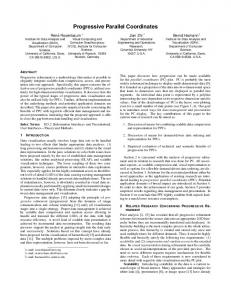
Figure 1: Meta Parallel Coordinates show the dimension-level view: The vertical axes represent the metrics while each polyline represents the value of the metrics for a given data dimension at any given timestep. Users can filter by a single dimension or multiple dimensions by making selections in the left panel. Specific time steps can also be selected by brushing.
To overcome these problems, we use visual abstraction in the form of screen-space metrics for creating an effective temporal summary that conveys the salient time-varying behavior with respect to all the data dimensions. Using these metrics, we build a meta parallel coordinates view (Figure 1) in which the metrics are represented by the vertical axes and each poly-line represents the values of those metrics for a color-coded data dimension, for a particular time step. Thus this view serves as a meta view for the conventional parallel coordinates display. We thus reduce the number of data points in the meta view, to d ∗ t = 1200 data points and thus we alleviate the scalability problem. The MPC is coordinated with the conventional parallel coordinates view (Figure 3) that shows the data plot for a particular time step. Interaction between the MPC and the conventional view enables a user to explore the data at multiple levels of granularity by seamlessly switching between exploring temporal changes at the dimension level, and then looking at the details, at the record level. This approach of separating the dimension level view (meta parallel coordinates) and the record level view (conventional parallel coordinates) is similar to that proposed by Turkay et. al. [16] who suggested a dual analysis model involving the dimension space and item space, by using standard statistical measures computed in the data space. In this work we use screen-space metrics, as they are computationally more efficient than purely data-based metrics. This is because after the initial data transformation the screen-space metrics are affected by only pixel resolution and are independent of the data cardinality.
Low entropy
High entropy
(a) Axis entropy indicates uniformity of a distribution.
High median density
Low median density
(b) Density median shows whether higher values or lower values dominate on an axis.
Clumped subspace
No clumping
(c) Clumped subspaces with high relative density on the left.
Figure 2: Semantic characteristics of visual structures that we quantify with screen-space metrics.
in coordination with the actual data view, the user can relate directly to the semantics of what the he/she sees on screen. In case of time-varying data, where one has to face multiple unknowns, this helps in accentuating the salient features in the data [1]. Several parallel coordinates variants have been proposed to deal with timevarying data [2, 4, 5, 11]. Our goal is to build derived, meta parallel coordinates views that guide the configuration of the conventional multivariate view.
Figure 3: Conventional Parallel Coordinates provide a record-level view: Here color gradient applied between a selected pair of axes (in this case, So kinetic Fe + + and kinetic S − −) and this serves as reference frame for analyzing the dominance of low and high values on the other dimensions.
1.2 Analytic Questions The following high-level questions guide the design and integration of the metrics and multiple views: • Q1 Can we visually detect dimensions that show the most salient patterns over a period of time? • Q2 How do we convey temporal change and integrate that information in different views of the data? 2 R ELATED W ORK A typical problem with traditional dimension reduction techniques like multi-dimensional scaling [13] is that transformation of data to a different space makes it difficult for users to understand the different patterns with respect to the original space. To preserve data fidelity better, we adopt the approach of Turkay et. al. [16] who suggested a dual analysis model involving the dimension space and item space. Quality metrics [15, 12], mostly based on the data space, in conjunction with axes-parallel projection techniques like parallel coordinates and the scatterplot matrix have been proposed to make the dimension selection/reduction process a user-centered one. We propose the use of screen-space metrics [7, 18] for investigating the properties of temporal data. Screen-space metrics are perceptually more beneficial as they are visually driven. The use of screen-space metrics belongs to the explicit encoding category [9] of enabling visual comparisons across objects. When used
3 M ETRICS The choice of metrics is motivated by Amar et al.’s recommendation [3] of general analysis tasks that a user performs with a visualization. Among those, characterizing univariate distribution and detecting hidden clusters in subspaces are relevant to this paper. Q1 and Q2 outlined in Section 1.2 are addressed by the metrics which are the basis for designing coordinated multiple views. The computation of the metrics is based on pixel-space axis histograms, in which the frequency of a pixel bin represents the number of lines starting or ending in the bin. The applicability of the metrics is not restricted to parallel coordinates, they can be applied directly to point-based representations like scatter plots. Axis Density: Two key indicators of the nature of a univariate data distribution are density (where, on the axis, most data values are located) and randomness (amount of disorder among the values). For the first criterion we compute the density median from the pixel histogram by finding the pixel coordinate of the bin that indicates the median value of the distribution. Higher density median indicates dominance of higher values on the axis, and correspondingly for lower values (Figure 2b). In terms of dispersion or data disorder, entropy [6] and variance are popular statistical measures. While there is no direct correlation between entropy and variance, it has been shown that entropy is more flexible in capturing dispersion as its location is independent of the mean, unlike variance [8]. The axis entropy is computed based on the frequency of each pixel bin in an axis histogram. In Shannon’s entropy formula [6] we use this frequency as the probability value to calculate entropy. The higher the entropy, the less informative is the distribution, as it implies most values have the same probability. The lower the entropy, the lesser uncertainty there is, and properties, like skewness of values in certain regions can be detected (Figure 2a). Subspace Density: If a distribution is multimodal, the median is not an accurate estimator of density. A multimodal distribution means data has a higher likelihood of being clumped (Figure 2c), i.e. highly concentrated at certain subspaces. The clumping factor helps indicate the subspace density. To compute the clumping factor we set first set a threshold value equal to the average over-plotting for a data dimension [7]. Then we iterate over all the pixel bins on an axis: if the frequency of a bin is equal to or greater than the threshold, we assign the bin to a cluster; when an adjacent pixel bin is found with frequency lower than the threshold, the
FeS UO2 FeS UO2 FeS UO2 FeS
1
FeS
kineticS-- FeS
11
kineticS-- FeS
2
kineticS--
3
Figure 4: Temporal variation of entropy for FeS (iron sulfite). First one shows uniform distribution implying high entropy, second one shows skewness signifying low entropy and the third one shows increasing randomness implying higher entropy.
FeS kineticFe
kineticFe
1
FeS kineticFe
2
FeS
3
Figure 5: Temporal variation of density median for kinetic Fe. Dominance of low values in the first one, followed by a mixture of low and high values in the second and then again a dominance of low values in the third one is captured by the density median.
2
3
4
UO2
Figure 6: Illustration of variation of clumping factor for different time steps: initially low clumping pattern between iron sulfide (FeS) and uraninite (UO2 ) changed to higher clumping at subsequent time steps indicated by the brushed lines.
cluster is cut off. Thus we get contiguous groups of clusters indicating dense subspaces. The clumping factor is then calculated by the sum of the number of pixel bins in all the clusters divided by the number of such clusters. The clumping metric is illustrated in Figure 6 where the clumped subspaces are shown by brushing. We can see that iron sulfide (FeS) initially shows low clumping factor, which increases in the subsequent time steps, as demonstrated by the dense clusters. 4 M ETA V IEW In contrast to the conventional parallel coordinates plot that serves as the data view, the meta view shows the values of the computed metrics and enables the user to build data views from them. The design of these views follows the visual information seeking mantra [14]: the meta view provides a global overview of the dimensions, and can be used to gain insights into the data before the user even looks at the details of the data view (conventional parallel coordinates) themselves. Henceforth, we will refer to the axes in the MPC as the metric dimensions and those in the conventional parallel coordinates view as the data dimensions. The three metric dimensions in the MPC are axis entropy, density median and clumping factor; while the last one is the time dimension. As shown in Figure 1, the different colors represent the different dimensions. Metrics are scaled globally so that values for different dimensions are comparable: the minimum and maximum for a given dimension for all time steps is computed first and then among those, we find the global minimum and maximum, that are used for scaling. There are 120 ∗ 10 = 1200 data points in the MPC. The user can reduce the number of data points in this view by selecting only a few data dimensions, as shown in Figure 6. The user can also load a specific number of time steps and filter through time steps of interest as shown in Figure 7. These interactive mechanisms help reduce clutter due to crossing of the lines and color-mixing among the lines. Some temporal trends are immediately visible in the MPC (Figure 1), like kinetic sulfate exhibiting very high density and variable clumping throughout and kinetic sulfide exhibiting high degree of variation on the entropy and density median axes. Dimensions selected from this view can be added to the time-varying conventional parallel coordinates plot (Figure 3). In the latter view, we use a con-
Figure 7: Brushing by time steps of interest in the MPC shows the behavior of the data dimensions with respect to multiple metrics. At a selected time step, high clumping between kinetic sulfate, sulfide and iron can be observed, as also the dominance of higher values on the sulfate and lower values on the sulfide.
tinuous color gradient from blue to orange, to indicate the transition from low to high values on an axis. The color gradient is applied on the left axis of an axis pair selected by a user, e.g., between the sorbed kinetic iron (So kinetic Fe++) and kinetic sulfide axes. The axis pairwise color gradient serves as a starting point for multivariate analysis: it enables one to see the multivariate behavior of the high and low values in one axis pair, with respect to all the other axes. 5 D ISCUSSION In this section, we describe some of the findings by the scientists (bioremediation experts), using our tool with respect to the analytic questions, Q1 and Q2. Finding dimensions of interest with respect to salient temporal patterns (Q1): The scientists were particularly interested in finding patterns for the sulfide compounds. The variations in entropy and density median helped them form and confirm many of their hypotheses. Figures 4 and 5 illustrate those for iron sulfide (FeS). As observed in Figure 4, an initial uniform distribution on the FeS axis is denoted by a high entropy value. Subsequently, the entropy drops, indicated by the skewness of the values. Then again, entropy begins to rise owing to more random patterns. The variations in density median are shown in Figure 5 where we see the rise and fall
of the median clearly depicted by the patterns. Lower data values dominate in the initial time steps, followed by the dominance of higher values, and then again a drop, all of which are indicated by the median. Conveying both overview and details of multivariate temporal patterns (Q2): To visualize multivariate patterns for the dimensions of interest, the scientists selected specific dimensions from the MPC to configure the conventional parallel coordinates plot. Moreover they filtered the data points by time steps in the MPC and visualized the behavior of multiple dimensions at a single time step. This is shown in Figure 7. The dimensions of interest are kinetic sulfate, kinetic sulfide, iron sulfide, kinetic iron, urananite, and tracer bromide. In particular, the scientists were interested in the interactions among kinetic sulfate, sulfide and iron, as indicated by the arrows. Towards the initial part of the reaction, as shown in Figure 7, both kinetic sulfate, sulfide iron show high clumping. This is reflected in the dense clusters in the parallel coordinates view. Also high sulfate values correspond to low sulfide and low tracer bromide values, and the dominance of the low values on the latter two dimensions is reflected by the low density median in the MPC. Advantages and Disadvantages: The advantages of using screenspace metrics are that after the initial histogram generation, they are only dependent on the screen size and independent of the data cardinality. Therefore for a time-varying dataset with high cardinality such as the bioremediation dataset, the computational complexity is significantly lowered. Moreover, compared to most of the earlier works in the area of time-varying data visualization, our approach is perceptually more beneficial as the visual structures are quantified by the metrics, and any structural change is also captured. The ability to investigate properties of subspaces is another added advantage of our approach. The user is an integral part of the analysis process as the MPC and the conventional parallel coordinates views can be used for a seamless transition between overview and details of temporal behavior. One drawback of our approach is that it is currently restricted to time-varying datasets with less than 10-15 dimensions, as a larger number of colors for the different dimensions would be difficult to differentiate. For datasets in which the number of dimensions is much higher, similar colors for dimensions could be picked based on similarity metrics [17]. Groups of dimensions that exhibit similar behavior would thus still be easy to spot in the meta views. 6
C ONCLUSION
In this paper, we have proposed a framework for meta parallel coordinates with multiple views that serve as an information-assisted model for facilitating a user-centric approach towards analyzing large, time-varying, high-dimensional data. Quantification of the visual structures and their integration with coordinated multiple views provides a perceptually beneficial approach towards facilitating efficient visual search for temporal patterns. As a next step we will incorporate more interactive features and apply the MPC framework on high-dimensional time-varying data from other domains. 7
ACKNOWLEDGEMENT
The research described in this paper is part of the Carbon Sequestration Initiative at Pacific Northwest National Laboratory (PNNL). It was conducted under the Laboratory Directed Research and Development Program at PNNL, a multiprogram national laboratory operated by Battelle for the U.S. Department of Energy. The authors thank Steve Yabusaki for providing the variably saturated flow and biogeochemical reactive transport simulations used in this paper. The data set used in this research was provided by the U.S. Department of Energy, Office of Science, Subsurface Biogeochemical Research Program through the Integrated Field Research
Challenge Site (IFRC) at Rifle, Colorado. The Rifle IFRC is a multi-institutional, multi-disciplinary project on subsurface biogeochemistry managed by the Lawrence Berkeley National Laboratory (LBNL). LBNL is operated for the U.S. Department of Energy by the University of California under contract DE-AC02-05CH11231 and Cooperative Agreement DE-FC02ER63446. R EFERENCES [1] W. Aigner, S. Miksch, W. Muller, H. Schumann, and C. Tominski. Visualizing time-oriented data–a systematic view. Computers & Graphics, 31(3):401–409, 2007. [2] H. Akiba and K. Ma. A tri-space visualization interface for analyzing time-varying multivariate volume data. In Proceedings of Eurographics/IEEE VGTC Symposium on Visualization, pages 115–122, 2007. [3] R. Amar, J. Eagan, and J. Stasko. Low-level components of analytic activity in information visualization. IEEE Symposium on Information Visualization, pages 111–117, 2005. [4] J. Blaas, C. Botha, and F. Post. Extensions of parallel coordinates for interactive exploration of large multi-timepoint data sets. Transactions on Visualization and Computer Graphics, 14(6):1436–1451, 2008. [5] M. Caat, N. Maurits, and J. Roerdink. Design and evaluation of tiled parallel coordinate visualization of multichannel eeg data. Visualization and Computer Graphics, IEEE Transactions on, 13(1):70–79, 2007. [6] T. Cover and J. Thomas. Elements of information theory. Wiley, 2006. [7] A. Dasgupta and R. Kosara. Pargnostics: Screen-space metrics for parallel coordinates. IEEE Transactions on Visualization and Computer Graphics, 16(6):1017–26, 2010. [8] N. Ebrahimi, E. Maasoumi, and E. Soofi. Ordering univariate distributions by entropy and variance. J. Econometrics, 90(2):317–336, 1999.
[9] M. Gleicher, D. Albers, R. Walker, I. Jusufi, C. Hansen, and J. Roberts. Visual comparison for information visualization. Information Visualization, 10(4):289–309, 2011. [10] A. Inselberg and B. Dimsdale. Parallel coordinates: A tool for visualizing multi-dimensional geometry. In IEEE Visualization, pages 361–378, 1990. [11] J. Johansson, P. Ljung, and M. Cooper. Depth cues and density in temporal parallel coordinates. In EuroVis, pages 35–42, 2007. [12] S. Johansson and J. Johansson. Interactive dimensionality reduction through user-defined combinations of quality metrics. Visualization and Computer Graphics, IEEE Transactions on, 15(6):993–1000, 2009. [13] I. Jolliffe. Principal component analysis, volume 2. Wiley, 2002. [14] B. Shneiderman. The eyes have it: A task by data type taxonomy for information visualizations. In Proceedings Visual Languages, pages 336–343, 1996. [15] A. Tatu, G. Albuquerque, M. Eisemann, J. Schneidewind, H. Theisel, M. Magnork, and D. Keim. Combining automated analysis and visualization techniques for effective exploration of high-dimensional data. In Symposium on Visual Analytics Science and Technology, pages 59– 66, 2009. [16] C. Turkay, P. Filzmoser, and H. Hauser. Brushing dimensions; a dual visual analysis model for high-dimensional data. Visualization and Computer Graphics, IEEE Transactions on, 17(12):2591–2599, 2011. [17] J. Wang, W. Peng, M. Ward, and E. Rundensteiner. Interactive hierarchical dimension ordering, spacing and filtering for exploration of high dimensional datasets. In IEEE Symposium on Information Visualization, 2003., pages 105–112. IEEE, 2003. [18] L. Wilkinson, A. Anand, and R. Grossman. High-dimensional visual analytics: Interactive exploration guided by pairwise views of point distributions. Visualization and Computer Graphics, IEEE Transactions on, 12(6):1363–1372, 2006.