Performance Improvement of Machine Learning via Automatic Discovery of Facilitating Functions as Applied to a Problem of Symbolic System Identification John R. Koza Computer Science Department Margaret Jacks Hall Stanford University Stanford, California 94305
[email protected] 415-941-0336
Martin A. Keane
James P. Rice
Third Millennium Venture Capital Limited 5733 Grover Chicago, Illinois 60630 312-777-1524
Abstract—The recently developed genetic programming paradigm provides a way to genetically breed a population of computer programs to solve problems. The technique of automatic function definition enables genetic programming to define potentially useful functions dynamically during a run – much as a human programmer writing a computer program creates subroutines to perform certain groups of steps which must be performed in more than one place in the main program. This paper finds an approximation to the impulse response function, in symbolic form, for a linear time-invariant system and demonstrates the value of automatic function definition in enabling genetic programming to accelerate the solution to this illustrative problem.
I. INTRODUCTION AND OVERVIEW A key goal in machine learning and artificial intelligence is to facilitate the solution of a problem by automatically and dynamically decomposing the problem into simpler subproblems. When a human programmer writes a computer program to solve a problem, he often creates a subroutine (procedure, function) enabling a common calculation to be performed without tediously rewriting the code for that calculation. For example, if a programmer needed to write a program for Boolean parity functions of several different orders, he might find it convenient first to write a subroutine for some lowerorder parity function. He would call on the code for this loworder parity function at different places and in different ways in his main program and combine the results to produce the desired higher-order parity function. Specifically, if the programmer were using the LISP programming language, he might first write a function definition for the odd-2-parity function xor (exclusive-or) as follows: (defun xor (arg0 arg1) (values (or (and arg0 (not arg1)) (and (not arg0) arg1)))).
This function definition (called a "defun" in LISP) does four things. First, it assigns a name, xor, to the function being defined thereby permitting subsequent reference to it. Second, this function definition identifies the argument list of the function being defined, namely the list (arg0 arg1) containing two dummy variables (formal parameters) called arg0 and arg1. Third, this function definition contains a
Stanford University Knowledge Systems Laboratory 701 Welch Road Palo Alto, California 94304
[email protected] 415-723-8405
body which performs the work of the function. Fourth, this function definition identifies the value to be returned by the function. In this example, the single value to be returned is emphasized via an explicit invocation of the v a l u e s function. This particular function definition has two dummy arguments, returns only a single value, has no side effects, and refers only to the two local dummy variables (i.e., it does not refer to any of the actual variables of the overall problem contained in the "main" program). However, in general, defined functions may have any number of arguments (including no arguments), may return multiple values (or no values), may or may not perform side effects, and may or may not explicitly refer to the actual (global) variables of the main program. Once the function x o r is defined, it may then be repeatedly called with different instantiations of its arguments from more than one place in the main program. For example, if the programmer needed the even-4-parity at some point in his main program, he might write (xor (xor d0 d1) (not (xor d2 d3))).
Function definitions exploit the underlying regularities and symmetries of a problem by obviating the need to tediously rewrite lines of essentially similar code. A function definition is especially efficient when it is repeatedly called with different instantiations of its arguments. However, the importance of function definition goes well beyond efficiency. The process of defining and calling a function, in effect, decomposes the problem into a hierarchy of subproblems. The ability to extract a reusable subroutine is potentially very useful in many domains. Consider the problem of discovery of a neural network to recognize a pattern presented as an array of pixels. Suppose the solution of a pattern recognition problem requires discovery of a particular feature (e.g., a line end) within the 3 by 3 pixel region in the upper left corner of an 8 by 8 array of pixels and also requires discovery of that same feature within a 3 by 3 pixel region in the lower left corner of the overall array. Existing neural net paradigms can successfully discover the useful feature among the nine pixels p11 , p12 , p13 , p21 , p22 , p23 , p31 , p32 , p33 in the upper left corner of a 8 by 8 array of pixels and can independently rediscover the same useful feature among the nine pixels p61 , p62 , p63 , p71 , p72 , p73 , p81 , p82 , p83 in the lower left corner of the overall array. But existing neural net paradigms do not provide a way to discover the common feature just once, to generalize the feature so that it is not
rigidly associated with particular pixels but is, instead, parameterized, and to then reuse the generalized feature detector to recognize occurrences of the feature in different 3 by 3 pixel regions within the array. That is, existing paradigms do not provide a way to discover a function of nine dummy variables just once and to call that function twice (once with p11, ..., p33 as arguments and once with p61, ..., p 83 as arguments). Such an ability would amount to discovering a nine-input subassembly of connections with appropriate weights, making a copy of the entire subassembly, implanting the copy elsewhere in the overall neural net, and then connecting nine different pixels as inputs to the subassembly in its new location in the overall neural net. Genetic programming provides a way to search the space of all possible functions composed of certain terminals and primitive functions to find a function which solves a problem. Automatic function definition enables genetic programming to define potentially useful functions, automatically and dynamically, and to then call them during a run – much as a human programmer creates subroutines (procedures, functions) to perform certain groups of steps which are repeatedly called from more than one place in the main program with different instantiations of its arguments. In this paper, we use genetic programming with automatic function definition to find the symbolic form of the impulse response function for a linear time-invariant system using only the observed response of the system to a particular known forcing function. The solution so discovered is then cross-validated with a number of other forcing functions not used during the learning process. Automatic function definition enables genetic programming to find an impulse response function with less computational effort. II. BACKGROUND ON GENETIC METHODS Since the invention of the genetic algorithm by John Holland [1975], the genetic algorithm has proven successful at finding an optimal point in a search space for a wide variety of problems [Goldberg 1989, Belew 1991, Davis 1987, Davis 1991, Michalewicz 1992]. However, for many problems the most natural representation for the solution to the problem is an entire function (i.e., a composition of primitive functions and terminals), not merely a single numerical point in the search space of the problem. The size, shape, and contents of the composition needed to solve the problem is generally not known in advance. In genetic programming, the individuals in the genetic population are compositions of primitive functions and terminals appropriate to the particular problem domain. These compositions of primitive functions and terminals correspond directly to the parse tree that is internally created by most compilers and to the programs found in programming languages such as LISP (where they are called symbolic expressions or S-expressions). The book Genetic Programming: On the Programming of Computers by Means of Natural Selection [Koza 1992a] describes the recently developed genetic programming
paradigm and demonstrates that populations of computer programs (i.e., compositions of primitive functions and terminals) can be genetically bred to solve a surprising variety of different problems in a wide variety of different fields. A videotape visualization of 22 applications of genetic programming can be found in the Genetic Programming: The Movie [Koza and Rice 1992]. III. STEPS REQUIRED TO EXECUTE GENETIC PROGRAMMING Genetic programming, like the conventional genetic algorithm, is a domain independent method. Genetic programming proceeds by genetically breeding populations of compositions of the primitive functions and terminals (i.e., computer programs) to solve problems by executing the following three steps: (1) Generate an initial population of random computer programs composed of the primitive functions and terminals of the problem. (2) Iteratively perform the following sub-steps until the termination criterion has been satisfied: (a) Execute each program in the population and assign it a fitness value according to how well it solves the problem. (b) Create a new population of programs by applying the following two primary operations. The operations are applied to program(s) in the population selected with a probability based on fitness (i.e., the fitter the program, the more likely it is to be selected). (i) Reproduction: Copy existing programs to the new population. (ii) Crossover: Create two new offspring programs for the new population by genetically recombining randomly chosen parts of two existing programs. The genetic crossover (sexual recombination) operation (described below) operates on two parental computer programs and produces two offspring programs using parts of each parent. (3) The single best computer program in the population produced during the run is designated as the result of the run of genetic programming. This result may be a solution (or approximate solution) to the problem. A. Crossover Operation The genetic crossover (sexual recombination) operation operates on two parental computer programs selected with a probability based on fitness and produces two new offspring programs consisting of parts of each parent. For example, consider the following computer program (LISP symbolic expression): (+ (* 0.234 Z) (- X 0.789)),
which we would ordinarily write as 0.234 Z + X – 0.789. This program takes two inputs (X and Z) and produces a floating point output. In the prefix notation used in Lisp, the
multiplication function * is first applied to the terminals 0.234 and Z to produce an intermediate result. Then, the subtraction function – is applied to the terminals X and 0.789 to produce a second intermediate result. Finally, the addition function + is applied to the two intermediate results to produce the overall result. Also, consider a second program:
+
*
+ Y
– X
*
* 0.789
Z
* Y
0.234
Z
(* (* Z Y) (+ Y (* 0.314 Z))),
which is equivalent to ZY (Y + 0.314 Z). In Fig. 1, these two programs are depicted as rooted, pointlabeled trees with ordered branches. Internal points (i.e., nodes) of the tree correspond to functions (i.e., operations) and external points (i.e., leaves, endpoints) correspond to terminals (i.e., input data). The numbers beside the function and terminal points of the tree appear for reference only. 1
1
+
*
2 3
4
0.234
Z
2
5
–
*
+
*
6
7
X
0.789
3
4
Z
6
Y
*
0.314
Z
9
ZY(Y + 0.314Z)
Fig. 1 Two Parental computer programs.
The crossover operation creates new offspring by exchanging sub-trees (i.e., sub-lists, subroutines, subprocedures) between the two parents. Assume that the points of both trees are numbered in a depth-first way starting at the left. Suppose that the point number 2 (out of 7 points of the first parent) is randomly selected as the crossover point for the first parent and that the point number 5 (out of 9 points of the second parent) is randomly selected as the crossover point of the second parent. The crossover points in the trees above are therefore the * in the first parent and the + in the second parent. The two crossover fragments are the two sub-trees shown in Fig. 2. +
*
Z 2
0.234Z Y
Y + 0.314Z + X – 0.789 Fig. 3 Two Offspring.
Thus, crossover creates new computer programs using parts of existing parental programs. Because entire sub-trees are swapped, this crossover operation always produces syntactically and semantically valid programs as offspring regardless of the choice of the two crossover points. Because programs are selected to participate in the crossover operation with a probability based on fitness, crossover allocates future trials to regions of the search space whose programs contains parts from promising programs.
7
Y 8
0.234Z + X – 0.789
5
0.314
IV. FINDING AN IMPULSE RESPONSE FUNCTION For many problems of control engineering, it is desirable to find a function, such as the impulse response function or transfer function (or an approximation to such functions), for a system for which one does not have an analytical model. The reader unfamiliar with control engineering should focus on the fact that we are searching the space of possible computer programs (i.e., functions) for a program which meets certain requirements. An approximation to the real target function is acceptable to the degree that the approximation generalizes. Fig. 4 shows a linear time-invariant system (plant) which sums the output of three major components, each consisting of a pure time delay element, a lag circuit containing a resistor and capacitor, and a gain element. For example, for the first component of this system, the time delay is 6, the gain is +3, and the time constant, R C , is 5. For computational simplicity and without loss of generality, we use the discrete-time version of this system in this paper. RC = 5
0.234
Z
Y
Delay = 6
*
Gain = +3 R C
0.314 0.234Z
Z
Y + 0.314Z
Input
RC = 12
These two crossover fragments correspond to the underlined sub-programs (sub-lists) in the two parental computer programs. The two offspring resulting from crossover are (+ (+ Y (* 0.314 Z)) (- X 0.789))
Gain = -8
Delay = 15
Fig. 2 Two Crossover Fragments
R C
Σ
Output
RC = 9 Delay = 25
Gain = +6
R C
and (* (* Z Y) (* 0.234 Z)).
The two offspring are shown in Fig. 3.
Fig. 4 Linear time-invariant system
In this problem, one is given the response of the unknown system to a particular specified forcing function – a unit
square input i(t) that rises from an amplitude of 0 to 1 at time 3 and falls back to an amplitude of 0 at time 23. The output of a linear time-invariant system is the discretetime convolution of the input i(t) and the impulse response function H(t). That is,
t
o(t) =
∑
i(t – τ ) H (τ ) . τ = –∞
The impulse response function H(t) for the system shown in Fig. 1 is known to be
0 if t < 6
0 if t < 1 5
0 if t < 2 5
Amplitude
+ + 1 1 1 3(1–5 )t– 6 –8(1–1 2) t– 15 6(1–9 ) t– 25 5 12 9 We now show how an approximation to this impulse response can be discovered via genetic programming using just the observed output from the square forcing function. The discrete-time version of the square input and the system's discrete-time response to it shown in Fig. 5 are the inputs for this problem; the goal is to find the impulse response shown in Fig. 6 or a good approximation to it. Plant Square Input Response 3
0 Plant Response Input -3 0
20
Time
40
60
Fig. 5 Plant square input response
Amplitude
0.6
0.0
-0.6 0
20
Time
40
60
Figure 6 Impulse response function
V.
PREPARATORY STEPS FOR USING GENETIC PROGRAMMING There are five major steps in preparing to use genetic programming, namely, determining (1) the set of terminals, (2) the set of primitive functions, (3) the fitness measure, (4) the parameters for controlling the run, and (5) the method for designating a result and the criterion for terminating a run. The first major step in preparing to use genetic programming is the identification of the set of terminals.
The individual impulse response functions in the population are compositions of the primitive functions and terminals. The single independent variable in the impulse response function is the time T. In addition, the impulse response function may contain various numerical constants. The ephemeral random floating point constant, ℜ, takes on a different random floating point value between –10.000 and +10.000 whenever it appears in the initial population and is explained in detail in Koza [1992a]. The second major step in preparing to use genetic programming is the identification of a sufficient set of primitive functions from which the impulse response function may be composed. For this problem, it seems reasonable for the function set to consist of the four arithmetic operations (addition, subtraction, multiplication, and division), the exponential function EXP, and the decision function IFLTE ("If Less Than or Equal"). Decision functions permit alternative calculations to be performed within a computer program and the exponential function seems relevant to this problem. Since genetic programming operates on an initial population of randomly generated compositions of the available functions and terminals (and later performs genetic operations, such as crossover, on these individuals), it is necessary to protect against the possibility of division by zero and the possibility of creating extremely large or small floating point values. Accordingly, the protected division function % ordinarily returns the quotient; however, if division by zero is attempted, it returns 1.0. The oneargument exponential function EXP ordinarily returns the result of raising e to the power indicated by its one argument. If the result of evaluating any function would be greater than 10 10 or less than 10-10 , then the nominal value 1010 or 10-10, respectively, is returned. The four-argument conditional branching function IFLTE evaluates and returns its third argument if its first argument is less than or equal to its second argument and otherwise evaluates and returns its fourth argument. The third major step in preparing to use genetic programming is the identification of the fitness measure for evaluating the goodness of an individual impulse response function in the population. For this problem, the fitness of an individual impulse response function in the population is measured in terms of the difference between the known observed response of the system to a particular forcing function and the response computed by convolving the individual impulse response function and the forcing function. The smaller the difference, the better. The exact impulse response of the system would have a difference of zero. The use of the convolution operation applied to the forcing function and the impulse response is a common technique used in control engineering to computer the time-doimain response. Specifically, each individual in the population is tested against a simulated environment consisting of N fc = 60 fitness cases, each representing the output o(t) of the given system for various discrete times between 0 and 59 when the square input i(t) described above is used as the forcing
function for the system. The fitness of any given genetically produced individual impulse response function G(t) in the population is the sum, over the Nfc = 60 fitness cases, of the squares of the differences between the observed response o(t) of the system to the forcing function i(t) (i.e., the square input) and the response computed by convolving the forcing function and the given genetically produced impulse response G(t). That is, the fitness is Nfc 2 t f(G) = o(t i ) – τ =∑– ∞i(t i – τ ) G (τ ) . i = 1
∑
The fourth major step in preparing to use genetic programming is the selection of values for certain parameters. Our choice of 4,000 as the population size and our choice of 50 as the maximum number of generations to be run reflect an estimate on our part as to the likely difficulty of this problem and the limitations of available computer time and memory. Our choice of values for the various secondary parameters that control the run of genetic programming (including the frequency of applying the genetic operations and our non-use of mutation) are the same default values as we have used on numerous other problems and are detailed in Koza [1992a]. Finally, the fifth major step in preparing to use genetic programming is the selection of the criterion for terminating a run and the method for designating a result. We designate the best-so-far individual as the result of a run. We terminate a run after 51 generations. VI. AUTOMATIC FUNCTION DEFINITION Automatic function definition can be implemented within the context of genetic programming [Koza 1992a, 1992d, Koza and Rice 1992]. This is accomplished by establishing a constrained syntactic structure for the individual S-expressions in the population. Each S-expression contains one or more function-defining branches and one or more "main" valuereturning branches. The value-returning branches may call the defined functions. The defined functions are defined in terms of dummy variables (formal parameters). For this problem, each individual S-expression in the population will have two branches. The first (leftmost) branch permits a one-argument function definition (defining a function called ADF0) and the second (rightmost) branch is the value-returning branch. Fig. 7 shows the overall structure of an S-expression with one function-defining branch and one value-returning branch. The first six types are invariant and appear above the horizontal dotted line in the figure. The function-defining branch appears in the left part of the figure and the valuereturning branch appears on the right. There are eight different "types" of points in this Sexpression. The first six types are invariant and appear above the horizontal dotted line in this figure. The eight types are as follows:
(1) the root of the tree (which consists of the place-holding PROGN connective function), (2) the top point, DEFUN, of the function-defining branch, (3) the name, ADF0, of the automatically defined function, (4) the argument list of the automatically defined function, (5) the VALUES function of the function-defining branch identifying, for emphasis, the value(s) to be returned by the automatically defined function, (6) the VALUES function of the result-producing branch identifying, for emphasis, the value(s) to be returned by the result-producing branch, (7) the body (i.e., work) of the automatically defined function ADF0, and (8) the body of the result-producing branch. PROGN DEFUN ADF0
Argument List
VALUES VALUES
Body of ADF0 Function Definition
Body of Value Returning Branch
Fig. 7 S-expression with one function-defining branch and one valuereturning branch
When the overall S-expression is evaluated, the PROGN sequentially evaluates the two branches. The first branch defines the automatically defined function ADF0 and does not return any value. The value returned by the overall Sexpression consists only of the value returned by the VALUES function associated with the value-returning branch. In preparing to use genetic programming with automatic function definition, we begin by deciding that there will be one defined function taking one dummy variable as its argument and that the independent variable of the problem, T, will be available to both the function definition and the valuereturning branch (i.e., it is a global variable). The terminal sets and function sets are different for the two branches of the structure. Specifically, the terminal set T 1 for the body of the function definition defining ADF0 (i.e., points of type 7) contains the dummy variable ARG0, so that T 1 = {T, ℜ, ARG0}, The function set F 1 for the function-defining branch is F1 = {+, -, *, %, EXP, IFLTE} taking 2, 2, 2, 2, 1, and 4 arguments, respectively. The terminal set T 2 for the body of the value-returning branch (i.e., points of type 8) does not contain the dummy variable ARG0 and is T 2 = {T, ℜ}. However, the function set F 2 for the value-returning branch contains the automatically defined function ADF0, so that F2 = {+, -, *, %, EXP, IFLTE, ADF0}.
Since a constrained syntactic structure is involved, we must create the initial random generation so that every individual Sexpression in the population has the syntactic structure presented above. Specifically, every individual S-expression must have the invariant structure represented by the six points of types 1 through 6 described above. The function-defining branch is a random composition of functions from the function set F 1 and terminals from the terminal set T 1 . The value-returning branch is a random composition of functions from the function set F 2 and terminals from the terminal set T 2. Moreover, since a constrained syntactic structure is involved, we must perform crossover so as to preserve the syntactic validity of all offspring as the run proceeds from generation to generation. Since each S-expression must have the invariant structure represented by the six points of types 1 through 6, crossover is limited to points from the body of the function definition of ADF0 (type 7) and points of the body of the value-returning branch (type 8). Structure-preserving crossover is implemented by allowing the selection of the crossover point in the first parent to be any point of types 7 or 8. However, once the crossover point in the first parent has been selected, the crossover point of the second parent must be of the same type. This restriction on the selection of the crossover point of the second parent ensures the syntactic validity of the offspring. In what follows, genetic programming will be allowed to evolve a function definition in the function-defining branch of each S-expression and then, at its discretion, to call the defined function in the value-returning branch. We do not specify what function will be defined in the function-defining branch. We do not specify what composition of terminals and functions will appear in the value-returning branch. We do not require that the defined function actually be invoked at all (it being possible to solve this problem via genetic programming without a function definition). We do not require that the function-defining branch actually use its available dummy variable. The structures of both the function-defining branch and the value-returning branch are determined by the combined effect, over many generations, of the selective pressure exerted by the fitness measure and by the effects of the operations of Darwinian fitness proportionate reproduction and crossover. VII. RESULTS FOR ONE RUN A review of one particular run will serve to illustrate how genetic programming progressively approximates the desired impulse response function. One would not expect any individual from the randomly generated initial population to be very good. In generation 0, the worst individual impulse response function among the 4,000 individuals in the population was equivalent to te3t. This sharply monotonically increasing function of T bears no resemblance to the correct impulse response of the system. Its fitness is the enormous value of 1.6 x 1077 (a low value being better). The median individual in the population was
equivalent to t + 8.354, a linear function of T, whose fitness is 2,249,945. The fitness of the best individual impulse response function was 101.03 (i.e., an average squared error of about 1.68 per fitness case). This best-of-generation individual program had 35 points (i.e., functions and terminals in the body of the function definition and body of the value-returning branch), has only one call to ADF0, and was (progn (defun adf0 (arg0) (values (* (+ (IFLTE T T ARG0 ARG0) (* T ARG0)) (* (EXP 4.152) (EXP 9.587))))) (values (% (IFLTE (% T 1.364) (EXP -2.113) (ADF0 T) (% -2.421 T)) (% (- T 6.653) (% T T))))).
When the defined function ADF0 is called with the argument T, it simplifies to 926370(t + t2), thereby making the value-returning branch equivalent to 1.0 if t = 0
-2.421 otherwise. t 2 – 6.653t By generation 15, the fitness of the best-of-generation individual had improved to 43.47. This individual has 36 points, has two calls to ADF0, and is shown below: (progn (defun adf0 (arg0) (values (% (- 7.732 ARG0) (* (IFLTE -5.295 -3.354 T 1.567) (EXP (* T -5.788)))))) (values (% (IFLTE (% T 1.364) (% (- T 6.653) (% T T)) (ADF0 T) (% -2.421 (ADF0 T))) (% T 1.364)))).
By generation 50, the best-of-generation individual shown below had 81 points, has two calls to ADF0, and a fitness value of 11.38 (i.e., an average squared error of only about 0.19 per fitness case) : (progn (defun adf0 (arg0) (values (% (- 6.511 T) (* (% (% (% (+ T ARG0) (- 5.141 -3.671)) (- 6.511 0.421)) (* (IFLTE -5.295 -3.354 T 1.567) (EXP (* T -5.788)))) (EXP (* T -5.788)))))) (values (% (IFLTE (% (- T 6.653) (% T (- T 6.653))) (% T 1.364) (IFLTE (% T 1.364) (% (- T 6.653) (% T T)) 1.364 (% -2.421 (ADF0 T))) (% -2.421 (ADF0 T))) (% (- T 6.653) (% T (% (% T 1.364) (% T (% T 1.364)))))))).
Since both calls to the defined function ADF0 are with the argument T, ADF0 simplifies to 1.0 if t ≥ 15
6.511 if t = 0
174.707 – 26.8328t otherwise thereby making the value-returning branch equivalent to 2.5377 if 25 < t < 4 7 t – 6.653
–4.5042 otherwise adf(t)[t – 6.653]
0
Fig. 10 presents two curves, called the "performance curves," relating to the problem of finding the impulse response function over a series of runs without automatic function definition. The curves are based on 18 runs with a population size M of 4,000 and a maximum number of generations to be run G of 51. 4 Generation 0 Square Input Response Amplitude
Amplitude
Note the subexpression (- 5.141 -3.671) which evaluates to 8.812. The needed value 8.812 was evolved, via subtraction, from the ephemeral random constants 5.141 and –3.671 over the generations. Fig. 8 compares (a) the genetically produced best-ofgeneration individual impulse response function from generation 50 and (b) the correct impulse response. As can be seen, the two curves are substantially similar. 1 Generation 50 Impulse Response
Correct Impulse Response Generation 50 Impulse Response
Plant Response Generation 0 -4 0 4
-1
20 Time 40 Generation 15 Square Input Response
60
60
Since the fitness measure (which is the driving force of genetic programming) is based on the response of the system to the square input, the performance of the genetically produced best-of-generation impulse response functions from generations 0, 10, and 50 can be appreciated by examining the time-domain response of the system to the square input. Fig. 9 compares (a) the plant response (which is the same in all three panels of this figure) to the square input and (b) the response to the square input using the best-of-generation individual impulse response functions from generations 0, 15, and 50. As can be seen in the first and second panels of this figure, the performance of the best-of-generation individuals from generations 0 and 15 was not very good, although generation 15 was considerably better than generation 0. However, as can be seen in the third panel of this figure, the performance of the best-of-generation individual from generation 50 is close to the plant response (the total squared error being only 11.38 over the 60 fitness cases). The ability of the genetically discovered impulse response function to generalize can be demonstrated by considering four additional forcing functions to the system – a ramp input, a unit step input, a shorter unit square input, and a noise signal. The best-of-generation individual from generation 50 produces a total squared error of only 6.38, 19.86, 12.59, and 6.40 over the 60 fitness cases to the plant response for these four different cross-validating forcing functions respectively. This evolved program therefore generalizes well. Note that since we are operating in discrete time, there is no generalization of the system in the time domain. FACILITATING VALUE OF AUTOMATIC FUNCTION DEFINITION Automatic function definition facilitates the finding of an impulse response function by reducing the amount of computational effort required to solve the problem. To demonstrate this, we first run this problem without automatic function definition over a series of runs to determine the computational effort necessary to yield a solution. We then make a series of runs of this problem with automatic function definition.
Amplitude
20 Time 40 Fig. 8 Generation 50 comparison
0 Plant Response Generation 15 -4 0 4
Amplitude
0
VIII.
0
20 Time 40 60 Generation 50 Square Input Response
0 Plant Response Generation 50 -4 0 20 Time 40 60 Fig. 9 Response of generations 0, 15, and 50 to square input
The rising curve in Fig. 10 shows, by generation, the experimentally observed cumulative probability of success, P(M,i), of solving the problem by generation i (i.e., finding at least one S-expression in the population which has a value of fitness of 20.00 or less over the 60 fitness cases). As can be seen, the experimentally observed value of the cumulative probability of success, P(M,i), is 11% by generation 25 and 61% by generation 46 over the 18 runs. The second curve (which first falls and then rises) in Fig. 10 shows, by generation, the number of individuals that must be processed, I(M,i,z), to yield, with probability z, a solution to the problem by generation i. I(M,i,z) is derived from the experimentally observed values of P(M,i). Specifically, I(M ,i,z) is the product of the population size M , the generation number i, and the number of independent runs R(z) necessary to yield a solution to the problem with probability z by generation i. In turn, the number of runs R(z) is given by log(1–z) R(z) = , log(1–P(M,i)) where the square brackets indicates the ceiling function for rounding up to the next highest integer. Throughout this paper, the probability z will be 99%.
[
]
Probability of Success (%)
100
8,000,000 46
P(M,i) I(M, i, z)
940,000
50
4,000,000
0
Individuals to be Processed
As can be seen, the I(M,i,z) curve reaches a minimum value at generation 46 (highlighted by the light dotted vertical line). For a value of P (M ,i) of 61%, the number of independent runs, R(z), necessary to yield a solution to the problem with a 99% probability by generation i is 5. The two summary numbers (i.e., 46 and 940,000) in the oval indicate that if this problem is run through to generation 46 (the initial random generation being counted as generation 0), processing a total of 940,000 individuals (i.e., 4,000 × 47 generations × 5 runs) is sufficient to yield a solution to this problem with 99% probability. This number, 940,000, is a measure of the computational effort necessary to yield a solution to this problem with 99% probability without automatic function definition. Fig. 11 shows performance curves for the same problem using automatic function definition based on 11 runs. The experimentally observed cumulative probability of success, P(M,i), is 18% by generation 25 and 82% by generation 47. The I(M,i,z) curve reaches a minimum value at generation 47. For a value of P(M,i) of 82%, the number of runs R(z) is 3. The two numbers in the oval indicate that if this problem is run through to generation 47, processing a total of 576,000 individuals (i.e., 4,000 × 48 generations × 3 runs) is sufficient to yield a solution to this problem with 99% probability using automatic function definition. The 576,000 individuals that must be processed to yield a solution using automatic function definition is considerably smaller than the 940,000 individuals required when automatic function definition is not used. That is, automatic function definition requires only about 61% as much computational effort.
0 0
25
50
Probability of Success (%)
100
8,000,000 P(M,i) I(M, i, z)
50
4,000,000 47
576,000
0
Individuals to be Processed
Generation Fig. 10 Performance curves showing that it is sufficient to process 940,000 individuals to yield a solution with 99% probability without automatic function definition
0 0
25
50
Generation Fig. 10 Performance curves showing that it is sufficient to process 576,000 individuals to yield a solution with 99% probability using automatic function definition
The average structural complexity of the 9 successful runs (out of the 11) with automatic function definition is 201 points as compared to an average of 224 points for the 11 successful runs (out of 18) without automatic function definition. IX. CONCLUSIONS We have demonstrated the use of genetic programming to genetically breed a good approximation to an impulse response function for a time-invariant linear system and also demonstrated that automatic function definition facilitated the solution of this problem. ACKNOWLEDGEMENTS Simon Handley of the Computer Science Department at Stanford University made helpful comments on this paper. REFERENCES Belew, Richard and Booker, Lashon (editors). Proceedings of the Fourth International Conference on Genetic Algorithms. San Mateo, CA: Morgan Kaufmann Publishers Inc. 1991. Davis, Lawrence (editor). Genetic Algorithms and Simulated Annealing. London: Pittman l987. Davis, Lawrence. Handbook of Genetic Algorithms. New York: Van Nostrand Reinhold 1991. Goldberg, David E. Genetic Algorithms in Search, Optimization, and Machine Learning. Reading, MA: Addison-Wesley l989. Holland, John H. Adaptation in Natural and Artificial Systems. Ann Arbor, MI: University of Michigan Press 1975. Revised Second Edition 1992 from The MIT Press. Koza, John R. Genetic Programming: On the Programming of Computers by Means of Natural Selection. Cambridge, MA: The MIT Press 1992. 1992a. Koza, John R. The genetic programming paradigm: Genetically breeding populations of computer programs to solve problems. In Soucek, Branko and the IRIS Group (editors). Dynamic, Genetic, and Chaotic Programming. New York: John Wiley 1992. 1992b. Koza, John R. Hierarchical automatic function definition in genetic programming. In Whitley, Darrell (editor). Proceedings of Workshop on the Foundations of Genetic Algorithms and Classifier Systems, Vail, Colorado 1992. San Mateo, CA: Morgan Kaufmann Publishers Inc. 1992. 1992d. Koza, John R. and Rice, James P. Genetic Programming: The Movie. Cambridge, MA: The MIT Press 1992. Michalewicz, Zbignlew. Genetic Algorithms + Data Structures = Evolution Programs. Springer-Verlag 1992.