PHASE-BASED GNSS DATA PROCESSING (PPP) WITH THE GPSTk. Salazar, D., Sanz-Subirana, J., and Hernandez-Pajares, M. Grupo de Astronomia y Geomatica (gAGE) Universitat Politecnica de Catalunya 08034 Barcelona Spain
[email protected]
Keywords: PPP GNSS data processing software GPSTk. Abstract The objective of this work is to show some of the advances made by the ’GPS Toolkit’ (GPSTk) project since the past “VII Semana Geomatica”, focusing in the data management strategy called ’GNSS Data Structures’ (GDS) and its associated data processing paradigm. The GDS allow for a clean, simple-to-read, simple-to-use software code that speeds up development and minimizes errors. Therefore, the geomatic researchers have a set of powerful but flexible tools at their disposal with which they can try novel approaches without devoting much time to data-management issues. The methodology to be used is to briefly describe the GDS paradigm, and to show how the different GNSS data ‘processing objects’ may be combined. The flexibility of this approach is then used to easily develop a fully working “Precise Point Positioning” (PPP) data processing chain, whose results favourably compare with other PPP-enabled software suites. 1
Introduction
The ”GPS Toolkit” (GPSTk) project is an advanced GNSS Open Source Software (GOSS) suite initiated by the Applied Research Laboratories of the University of Texas (ARL:UT), aiming to provide a world class GNSS library computing suite to the satellite navigation community. One of its main goals is “to free researchers to focus on research, not lower level coding” [1]. Currently it is actively maintained by more than a dozen developers around the world using the Internet as communication medium. Development facilities are provided by the popular SourceForge open source application repository. The initial code of the GPSTk was released in summer 2004 and presented at the ION-GNSS-2004 [2], and its functionality has been continuously improving. A very brief list of the tools provided by the GPSTk includes: Handling of observation data and ephemeris in RINEX and SP3 formats, antenna data in Antex format, mathematical, statistical, Matrix and Vector algorithms, time handling and conversions, ionospheric and tropospheric models, cycle slip detection and correction, solid tides, ocean loading and pole tides models, etc. As a typical Open Source project, it is open to any researcher or institution because it is released under the GNU LGPL license, which allows freedom to develop both commercial and non-commercial software. GPSTk is highly platform-independent because it uses ANSI C++. It is reported to run on operative systems like Linux, Solaris, AIX, MS Windows and Mac OS X. It may be compiled using several free and commercial compilers, both in 32 bits and 64 bits platforms. Also, some parts of it are reported to run in platforms such as the Nokia 770 Internet Tablet and the Gumstix line of full function minicomputers [3]. The GPSTk software suite consists of a core library and extra applications. The library provides several functions that solve processing problems associated with GNSS (for instance, using RINEX files), and it is the basis for more advanced applications distributed as part of the GPSTk suite. This work focus in library provisions to write clean, simple-to-read, simple-to-use software code that speeds up development
and minimizes errors, enabling at the same time to implement “Precise Point Positioning” processing [4]. 2
GNSS Data Structures approach and processing paradigm
After developing the basic code-based GNSS data processing, and starting to add phase-based capabilities to the GPSTk, several project developers came to the conclusion that some kind of hierarchy of data structures should be added in order to easily cope with frequent data management situations that were very difficult to deal with when using just vectors and matrices. For instance, let’s consider that the typical GNSS data post-processing starts reading data from Rinex files. In case this file is from observations, apart from C1, L1, etc, the programmer must take care of metadata such as epoch and cycle slip receiver flags. If the file contains ephemeris, these must be properly stored and organized. In the following processing steps, a lot of extra information must be computed from the original data: Observable combinations, satellite’s arc numbers, elevation, azimuth, relativistic, tropospheric and ionospheric corrections, wind-up effects and antenna phase center variations are just a few. Besides, all this extra information must be properly catalogued and cross-referenced according to, for instance satellite, receiver, data type and epoch each data piece is related to. Writing software that appropriately keeps track of all these relationships is no easy task, and the ensuing complexity makes it very difficult to debug, maintain, and enhance. As an answer to these data management issues, a new and flexible set of data structures, called the ’GNSS Data Structures’ (GDS) were added to the GPSTk. These structures hold several kinds of GNSS-related data, properly indexed by station, epoch, satellite and type, and store them efficiently. In this way, both the data and corresponding metadata is preserved, and data management issues are properly addressed. Details about the GDS design and implementation may be found on [5], as well as in the GPSTk project website [1]. In summary, GDS take advantage of the observation that several types of GNSS-related data structures share some common characteristics, and thence they can be modelled in an unified way, creating structures that index each data value with four different indexes. Those four indexes are implemented in the GPSTk as C++ classes SourceID, SatID, TypeID, and DayTime. Objects associated with these classes provide the GNSS programmer with a large set of methods to work with them in an easy way. Please refer to GPSTk Application Programming Interface (API) document for further details [6]. Apart from the GDS themselves, a “GDS processing paradigm” was also developed, where GNSS data processing becomes like an ’assembly line’, and the GDS are treated like ’white boxes’ that ’flow’ from one ’workstation’ to the next in this ’assembly line’. It is important to note here that most of the GDS-related classes presented in this work currently are only available in the development branch of the GPSTk. Please follow the instructions in the GPSTk website to download this branch. 3
Some simple GDS examples
In order to quickly harness the power of this approach, some simple examples are presented. In the first one, we’ll just extract a single epoch worth of data out of a Rinex observation file and get that data into a GDS: Line #1 declares an object of class RinexObsStream, which is used to handle Rinex observation files. That object receives in this case the name of rinexFile, and will take care of ‘ebre0300.02o’ Rinex file.
1 2
RinexObsStream rinexFile("ebre0300.02o"); gnssRinex gpsData;
3
rinexFile >> gpsData;
On the other hand, line #2 declares an object of class gnssRinex, which is a very handy GNSS Data Structure. Our data will be stored in this object, which will be called gpsData. Finally, line # 3 does the real work: It will take one epoch of data out of rinexFile (file ‘ebre0300.02o’, indeed), and will pour it into gpsData;. No more code is needed for this action, and line # 3 is referred to as the “processing line”. Please note how the C++ operator >> is used to convey the idea that data “flows” out of the Rinex file into the GDS “box” that will carry it around. The statement rinexFile >> gpsData; has the additional property that it is evaluated as TRUE if operation is completed without problems, and as FALSE otherwise (for instance, when end of Rinex file is reached). The aforementioned property allows us to slightly modify the former example to get a much more useful behavior: 1 2
RinexObsStream rinexFile("ebre0300.02o"); gnssRinex gpsData;
3
while( rinexFile >> gpsData ) { ... your GNSS data processing code here ... }
4
In this case the while loop will repeat itself until end of Rinex file is reached, and in each repetition a single epoch data set of Rinex observations is encapsulated into gpsData, and is fully available to the researcher to process it. 3.1
Code-processing example
Now a code-processing example will be presented. For space reasons most of the initialization phase is skipped, so you must refer to GPSTk API to get the fine details. Also, the GPSTk provides carefully explained examples: Look at “example6.cpp” and “example7.cpp” in “examples” directory for code-based processing with GDS and the GPSTk. We will start the example with the lines handling ephemeris data: 1 2 3
RinexNavStream rnavin("bahr1620.04n"); RinexNavHeader rNavHeader; rnavin >> rNavHeader;
4 5 6 7
IonoModel ioModel; ioModel.setModel(rNavHeader.ionAlpha, rNavHeader.ionBeta); IonoModelStore ionoStore; ionoStore.addIonoModel(DayTime::BEGINNING_OF_TIME, ioModel);
8 9 10 11 12
RinexNavData rNavData; GPSEphemerisStore bceStore; while (rnavin >> rNavData) { bceStore.addEphemeris(rNavData); }
Lines #1 to #2 declare objects to take care of ephemeris Rinex files and associated header. Line #3 then reads the header and store it. Please remember that Klobuchar ionospheric coefficients are stores in ephemeris Rinex header, so this step is important for lines #4 to #7.
The first two of them then declare an “ionospheric model” object (IonoModel) and fill it with Klobuchar coefficients, and after that declare a ionospheric model store (ionoStore) and push in the previously defined model. Please note that this approach allows to store models for multiple days. After that, the ephemeris data is read and stored in a proper object, which is filled with all available ephemeris data, one epoch at a time, in a way similar as was already explained for observation data. 13
Position nominalPos(3633909.1016, 4425275.5033, 2799861.2736);
14
MOPSTropModel mopsTM( nominalPos.getAltitude(), nominalPos.getGeodeticLatitude(), 162 );
15
ModelObs gpsModel( nominalPos, ionoStore, mopsTM, bceStore, TypeID::C1);
16
SolverLMS solver;
17 18
RinexObsStream rinexFile("ebre0300.02o"); gnssRinex gpsData;
Line #13 declares the nominal position of receiver, line #14 setup a tropospheric model (there are several available), and line #15 then takes care of a very interesting object: A “modeler”. This “modeler” object (gpsModel) takes as input the nominal receiver position, ionospheric and tropospheric models, ephemeris data and type of observable it will work with, and will carry up the tasks related with GPS data modelling, computing all the delays defined by the GPS standards and using them to compute the prefit residuals and geometric coefficients that will later be used by the solver. All this wealth of information will be inserted in the GDS at due time. Then, line #16 declares the “solver”, the object in charge of building and solving the equation system. In this case it uses a simple Least Mean Squares solving algorithm (there are others available). The function of lines #17 and #18 was already described. Finally, we present the final while loop that extracts Rinex data, runs the GPS model, solves the navigation equations and prints the results: 19
while( rinexFile >> gpsData ) {
20
gpsData >> gpsModel >> solver;
21 22 23
cout gpsModel becomes again gpsData, where the new gpsData is a superset of the original. Therefore, the second part of line #20 then becomes gpsData >> solver, and solver object will find in gpsData all the information it needs to build and solve the navigation equation system. This approach to GNSS data processing is called the “GDS processing paradigm”, where the GDS processing becomes akin to how a car is built in a car factory. The GDS (like the car) “flows from one “workstation” to the next, where in this particular case the “workstations” are represented by objects from “processing classes” ModelObs and SolverLMS. From the developer (and researcher) point of view, the GDS is just like a “box” (a “white box”, indeed) that holds and automatically organizes all the information needed, in his only concern is to push this “box” through all the “processing classes” he needs to. This process, which may seem computationally complex and convoluted at first sight, is however efficiently implemented using the C++ Standard Template Library (STL). A Rinex observation file (at 30 s data rate) of a full day processed in this way takes less than 0.2 seconds in an average laptop PC with Linux 1 . Coming back to our code-based processing example, the final lines #21 to #23 just take care of printing the solution to the screen, using the standard C++ cout printing object. Please take note of the handy way to get solution values out of solver objects, which represents the consistent way to refer to data types along all the GDS processing paradigm. 4
PPP data processing accessory classes
PPP implementation is a complex task, and issues like wind-up effect, solid, oceanic and polar tides, antenna phase centers, etc. must be taken into account. Also, precise satellite orbits and clocks are used in PPP, but these products are usually provided each 900 s, while observations are usually provided each 30 s. Thence, some time management issues also arise. We will start presenting some accessory classes that ease these complex issues. However, take into account that, again, most initialization details are skipped. For complete phase-based processing implementations please read “example8.cpp”, “example9.cpp” and “example10.cpp” in the GPSTk development repository. The GPSTk API is also a mandatory read. 4.1
Handling configuration files
Given the potentially high number of PPP processing parameters involved, reading configuration files is an important ability in order to avoid recompilation of source code each time we want to change a given parameter. The GPSTk provides ConfDataReader, a powerful class to parse and manage configuration data files. It supports multiple sections, variable descriptions and value descriptions (such as units), and a wide range of variable types. Given a configuration file named “configuration-file.txt”, whose content is:
1 The former figure disregards output time. Redirecting output to a file in the laptop hard disk raises the overall processing time to about 0.7 seconds.
# Default section tolerance, allowed difference between time stamps = 1.5, secs [BELL] reference = TRUE
Then a typical way to use this class follows: 1 2
ConfDataReader confRead; confRead.open("configuration-file.txt");
3 4 5
double tolerance = confRead.getValueAsDouble("tolerance"); cout > gpsData ) { try {
3
gpsData >> ... >> decimateData >> ...
4 5 6 7 8 9 10 11 12 13 14 15 16 17
5
} catch(DecimateEpoch& d) { continue; } catch(Exception& e) { cout
requireObs >> linear1 >> markCSLI >> markCSMW markArc >> decimateData >> basicModel >> eclipsedSV grDelay >> svPcenter >> corr >> windup computeTropo >> linear2 >> pcFilter >> phaseAlign linear3 >> baseChange >> cDOP >> pppSolver;
The GDS processing data chain is indeed a single C++ line, although in this case (for clarity sake) spans from line #1 to line #5. Also, all this line must be enclosed within a while loop to process all available epochs, and within a try - catch block to manage exceptions. Several of these objects need initialization, but that part is omitted here. Again, please consult GPSTk examples and API. Table 1 summarizes object names, classes they belong to, and purpose. Particular mention deserves object pppSolver, belonging to SolverPPP class. This object is preconfigured to solve the PPP equation system in a way consistent with [4]: Coordinates are treated as constants (static), receiver clock is considered white noise, and vertical tropospheric effect is processed as a random walk stochastic model. Figure 1 plots the results for former PPP processing code applied to station MADR, May 27th., 2008. As mentioned, the positioning strategy is the default one for SolverPPP objects: PPP with static coordinates. These results are consistent with what is expected from these processing strategies, showing a small residual bias in the “Up” coordinate of about 17 millimeters. Those pre-assigned stochastic models may be tuned and even changed at will, given that they are objects inheriting from general class StochasticModel. In this regard, a way to check how good GPSTk PPP modelling is consists in treating coordinates as white noise (kinematic). The former is achieved during initialization phase in a very simple way: 1 2
WhiteNoiseModel newCoordinatesModel(100.0); pppSolver.setCoordinatesModel(&newCoordinatesModel);
Now, pppSolver object will consider both coordinates and receiver clock as white noise stochastic variables, while vertical tropospheric effect is still treated as a random walk process. The coordinates’ model has an
OBJECT
CLASS NAME
PURPOSE
requireObs
RequireObservables
Check if required observations are present
linear1
ComputeLinear
Compute linear combinations used to detect cycle slips
markCSLI
LICSDetector2
Detect and mark cycle slips using LI combination
markCSMW
MWCSDetector
Detect and mark cycle slips using Melbourne-Wubbena combination
markArc
SatArcMarker
Keep track of satellite arcs
decimateData
Decimate
If not a multiple of 900 s, decimate
basicModel
BasicModel
Compute the basic components of a GNSS model
eclipsedSV
EclipsedSatFilter
Remove satellites in eclipse
grDelay
GravitationalDelay
Compute gravitational delay
svPcenter
ComputeSatPCenter
Compute the effect of satellite phase center
corr
CorrectObservables
Correct observables from tides, antenna phase center, etc.
windup
ComputeWindUp
Compute wind-up effect
computeTropo
ComputeTropModel
Compute tropospheric effects
linear2
ComputeLinear
Compute ionosphere-free combinations PC and LC
pcFilter
SimpleFilter
Filter out spurious data in PC combination
phaseAlign
PhaseCodeAlignment
Align phases with codes
linear3
ComputeLinear
Compute code and phase prefit residuals
baseChange
XYZ2NEU
Prepare data to use North-East-UP reference frame
cDOP
ComputeDOP
Compute DOP figures
pppSolver
SolverPPP
Solve equations with a Kalman filter configured in PPP mode
Table 1: PPP processing objects and classes.
assigned sigma of 100.0 meters (see last part of line # 1). Figure 2 presents the results for this type of processing, confirming the good quality of GPSTk model (results are consistently within +/- 10 cm from nominal value).
Figure 1: Static PPP positioning error regarding IGS nominal. MADR station, 2008/05/27. 5.1
Forward-Backward Kalman Filter
Previous results were obtained with a Kalman filter that only used information from the “past”. However, PPP is done in post-process, and thence the filter could also use information from the “future” as well from the past. This is usually done running the filter in forward-backward mode, where the filter takes advantage of ambiguity convergence achieved in the previous forwards run, and uses that information for the next backwards run. This process may be iterated at will. An object of class SolverPPPFB is used to achieve this. This class encapsulates SolverPPP class functionality and adds a data management and storage layer to handle the whole process. From the user’s point of view, the main change is to replace SolverPPP object (pppSolver) with a new SolverPPPFB object (fbpppSolver, for instance) inside the while loop reading and processing RINEX data file. After the first forwards processing is done (and data is internally indexed and stored), it is simply a matter of telling fbpppSolver object how many forward-backward cycles we want it to “re-process”. For instance, to carry out 4 forward-backward additional cycles: fbpppSolver.ReProcess(4);
After that, one last forwards processing is needed to get the time-indexed solutions out of fbpppSolver. Please note that in this case the solution is given in a NEU reference frame instead of ECEF. To achieve that we must tell so to the solver object when declaring it, and insert a XYZ2NEU object in the processing
Figure 2: Kinematic PPP positioning error regarding IGS nominal. MADR station, 2008/05/27. 1 2 3 4 5
while( fbpppSolver.LastProcess(gpsData) ) { cout