Physics-Based Modeling for Heterogeneous Objects - Computational

Physics-Based Modeling for Heterogeneous Objects Xiaoping Qian e-mail: [email protected]

Debasish Dutta e-mail: [email protected] Department of Mechanical Engineering, The University of Michigan, Ann Arbor, MI 48105

1

Heterogeneous objects are composed of different constituent materials. In these objects, material properties from different constituent materials are synthesized into one part. Therefore, heterogeneous objects can offer new material properties and functionalities. The task of modeling material heterogeneity (composition variation) is a critical issue in the design and fabrication of such heterogeneous objects. Existing methods cannot efficiently model the material heterogeneity due to the lack of an effective mechanism to control the large number of degrees of freedom for the specification of heterogeneous objects. In this research, we provide a new approach for designing heterogeneous objects. The idea is that designers indirectly control the material distribution through the boundary conditions of a virtual diffusion problem in the solid, rather than directly in the native CAD (B-spline) representation for the distribution. We show how the diffusion problem can be solved using the B-spline shape function, with the results mapping directly to a volumetric B-Spline representation of the material distribution. We also extend this method to material property manipulation and time dependent heterogeneous object modeling. Implementation and examples, such as a turbine blade design and prosthesis design, are also presented. They demonstrate that the physics based B-spline modeling method is a convenient, intuitive, and efficient way to model object heterogeneity. 关DOI: 10.1115/1.1582877兴

Introduction

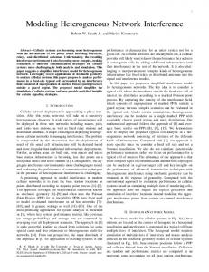
Heterogeneous objects are made of different constituent materials and/or have continuously varying material composition thus producing gradation in their material properties. They are sometimes known as functionally gradient materials 共FGM兲. In these objects, different materials can be mixed and varied to satisfy multiple or even conflicting design requirements, and they possess many desired material properties, which cannot be obtained otherwise. Over the past decade, the uses of heterogeneous objects have grown into many fields. When the FGM concept was first introduced, two dissimilar materials such as metal and ceramic were combined to relieve thermal stress. Now the applications of heterogeneous objects span from aerospace, nuclear energy, chemical plant, and biomedical engineering, to general commodities. For example, a graded interface for bone in orthopedic implants is shown in Fig. 1. Conventional methods of fixing an artificial bone and joint prosthesis to bone include the following steps: total close contact of the prosthesis to the bone, direct mechanical fixation with screws or spikes, and filling the space between the prosthesis and bone with polymethylmethacrylate 共PMMA兲 bone cement. However, this causes pain to the patient during weight bearing situations such as walking because there is micromotion of the prosthesis within the bone, and subsequently the prosthesis may even loosen in the bone. As a result, the breaking of such fixation frequently occurs. A more effective method for adhering prosthesis to the bone is to coat it with a porous metal because new bone ingrowth into the pores occurs after implantation. A graded layer of hydroxyapatite 共HAp兲 is coated on the porous metal. It bonds to the bone physicochemically, thereby increasing the adhesion strength and rate of binding to the bone. Therefore, porous metal with a HAp coating remedies the big drawbacks of cementless prosthesis. It prevents pain to the patient while walking caused by micromotion or loosening of a prosthesis fixed without bone cement, and also allows weight bearing earlier after implantation 关1兴. Contributed by the Design Automation Committee for publication in the JOURNAL OF MECHANICAL DESIGN. Manuscript received Aug. 2001; rev. Nov. 2002. Associate Editor: J. E. Renaud.

416 Õ Vol. 125, SEPTEMBER 2003

Figure 1 is a schematic structure of such an FGM interface. This FGM region is composed of porous titanium plus hydroxyapatite 共HAp兲. Ti has good mechanical toughness and HAp has good biocompatibility. The uniform combination of Ti and HAp would cause bio-incompatibility and weakened strength due to the material property differences. Such material property differences are resolved by using a mixture of Ti and HAp with varying proportions. The sharp interface between Ti and HAp is eliminated through a graded zone of Ti/HAp. The bending strength of the resulting material is similar to human bone. The figure also shows typical variation in properties due to the variation in material composition at the FGM region. As evidenced in the prosthesis design example, heterogeneous objects have many advantages over objects composed of uniform materials. Such advantages have brought to the forefront the research on heterogeneous objects realization. In the last decade, optimal design techniques such as the homogenization design method have been developed which create just such heterogeneous objects 关2兴. Also, in the last few years, layered manufacturing 共LM兲 has matured significantly and is capable of fabricating heterogeneous objects 关3兴. In layered manufacturing, a part is built by selectively depositing materials layer-by-layer under computer control. A critical link between the design and fabrication of such heterogeneous objects is heterogeneous object modeling, a task creating the heterogeneous object model that can be used for the design, analysis and fabrication of heterogeneous objects. The recent research on heterogeneous object modeling has been primarily focused on the representation schemes, i.e., using mathematical model and computer data structures to represent the geometry and material composition of heterogeneous objects. Nonetheless, limited means are available for specifying and controlling the material composition in the heterogeneous object model. One of the main challenges lies in the fact there exist a large number of degrees of freedom to completely define a heterogeneous object. For example, for a 3d object with m types of materials and n number of variations for each material, the modeling space is E 3 ⫻n m dimensional. To specify material composition within such a complex space, an effective and efficient method is crucial. This paper presents a diffusion process based method for het-

Copyright © 2003 by ASME

Transactions of the ASME

Table 1 Comparison of heterogeneity modeling methods Methods Control points Analytical functions Voxel Implicit functions

Fig. 1 Schematic structure of an FGM interface within prosthesis

erogeneous object modeling. It provides a convenient, intuitive and efficient way to specify material compositions within the heterogeneous objects. In the rest of this paper, Section 2 reviews the previous research on heterogeneous object modeling. Section 3 presents the volumetric B-spline representation for heterogeneous objects. Section 4 describes the mathematical model for a diffusion process. Section 5 details the mathematical formation for the diffusion based B-spline heterogeneous object modeling. Section 5.2 extends the method to time dependent heterogeneous objects. Method for imposing constraints on the diffusion model is presented in Section 6. The implementation and examples are shown in Section 7. Finally, the paper is concluded in Section 8. 2 Previous Research. Kumar and Dutta proposed R-m sets could be used for representing heterogeneous objects 关4兴. Jackson proposed another modeling approach based on subdividing the solid model into sub-regions and associating the analytical composition blending functions with each region 关5兴. Some other modeling and representation schemes, utilizing either voxel model, implicit functions or texturing, have also been proposed 关6 – 8兴. Unlike the above research focusing on geometry/material representation schemes, in this paper, we specifically focus on the methods for specifying material variation. In each of the aforementioned representation schemes, they used different modeling methods. In terms of material specification, we classify these methods into the following four categories: control points based, analytical functions based, implicit functions based, and voxel based modeling methods. It should be noted that these methods do Journal of Mechanical Design

Model Coverage

Operation Convenience

Excellent Poor Excellent Poor

Poor Excellent Poor Excellent

not necessarily associate with a particular representation scheme. For example, both control points based and analytical functions based methods can be applied in R-m set based representation scheme for heterogeneous objects. Therefore, the advantages and disadvantages of heterogeneity specification methods do not naturally reflect the advantages and disadvantages of each representation scheme. A comparison of these object heterogeneity specification methods is shown in Table 1. In this table, model coverage refers to the coverage of geometry and material variation each method can model. The convenience refers to the convenience level for users to specify and change the material heterogeneity. A control point based method models the object heterogeneity by specifying values of a set of control points and interpolating them with the shape functions, such as B-spline 关9兴, Bezier 关5,10兴, or NURBS 关6兴. Due to the large number of control points, such a method has excellent representation coverage, but for the same reason it is not convenient to use. An analytical function based method represents the object heterogeneity by explicit functions rather than control point based functions 关4,11兴. This method is particularly popular in functionally gradient materials research community where an explicit function, e.g., linear, parabolic, or exponential, is used to represent the volume fraction at each point of an object 关12兴. Using such a method, it is easy to manipulate the material composition but it has limited model coverage. A voxel based method represents material heterogeneity in terms of discretized voxel in the object. For example, voxel-based multi-material object is proposed in 关6兴. Such a method has advantages, such as relatively wide representation coverage. It is also good for visualization. However, due to its large size of voxels in 3 dimensional objects, it is inconvenient and inefficient to manipulate and control the heterogeneity. An implicit function based method models the heterogeneity in the form of implicit functions. i.e., f (m)⫽0. For example, implicit functions can be constructed for an R-function method 关7兴. For complicated or arbitrary geometry boundary, it is difficult to construct such implicit functions. Due to the implicit nature, such methods are not good for anticipating the heterogeneity variation during design modifications, a task that needs to be supported. Therefore, the current methods for specifying material composition face a trade-off between the model coverage and operation convenience. To obtain overall desirable performance in model coverage, convenience and efficiency of heterogeneous object modeling, we propose physics-based heterogeneous object modeling. In this paper, we use a virtual diffusion process to model the heterogeneity at each point. Mathematically, we extend the B-spline to represent the heterogeneous objects. We use the second order differential equation for the diffusion process to generate the material composition distribution. Conceptually, only a few parameters, carrying physical implications, and constraints are used to intuitively manipulate the material composition. For the interests of simplicity, we refer to object heterogeneity as material composition in this paper, even though the method presented in this paper applies to other object heterogeneity as well, such as temperature distribution and stress field. It should be noted that this work was in part inspired by the physics based modeling of geometry 关13–15兴, where the Lagrange dynamic model is used for modeling the geometry deformation. SEPTEMBER 2003, Vol. 125 Õ 417

Fig. 2 Tensor product B-spline volume

3

B-Spline Representation for Heterogeneous Objects

Tensor product solid representation has been widely used in computer aided geometric design community. Under the context of heterogeneous objects, relevant proposals based on tensor product volumes have also been reported 关5,6,9兴. In this paper, B-spline tensor representation is used to represent material composition and material properties in heterogeneous objects. It is also extended to represent the time dependent heterogeneous objects. We choose B-spline representation for heterogeneous objects simply to shorten the computational time. There is no technical difficulty to extend the methodology to a NURBS volume. 3.1 B-Spline Tensor Solid Representation for Heterogeneous Objects. For each point (u, v ,w) in the parametric domain of a tensor product B-spline volume V 共Fig. 2兲, there is a corresponding point V(u, v ,w) at Cartesian coordinates (x,y,z) with material composition M, noted as (x,y,z,M ). We define such a B-spline volume as: n

V 共 u, v ,w 兲 ⫽

m

l

兺兺兺N i⫽0 j⫽0 k⫽0

i, p 共 u 兲 N j,q 共 v 兲 N k,r 共 w 兲 P i, j,k

(1)

Where P i, j,k ⫽(x i, j,k ,y i, j,k ,z i, j,k ,M i, j,k ) are control points for the heterogeneous solid volume. N i, p , N j,q , and N k,r are the pthdegree, qth-degree, and r th-degree B-spline functions defined in the direction of u, v , w respectively. For example, N i, p (u), the i-th B-spline basis function of p-degree 共order p⫹1), is defined as: N i,0共 u 兲 ⫽ N i,p 共 u 兲 ⫽

再

1

if u i ⭐u⭐u i⫹1

0

otherwise

u⫺u i u i⫹ p⫹1 ⫺u N N 共 u 兲⫹ 共u兲 u i⫹ p ⫺u i i, p⫺1 u i⫹ p⫹1 ⫺u i⫹1 i⫹1,p⫺1

3.2 Representation for Material Properties of Heterogeneous Objects. Due to the material gradation in heterogeneous objects, the material properties also exhibit variation. For designers, controlling heterogeneous object’s properties is more useful and intuitive than controlling the material composition. In order to control material properties, an effective representation is needed. The relationship between material properties and the composition has been extensively studied 关12兴. For example, Eq. 共2兲 and Eq. 共3兲 give the approximate relationships of thermal conductivities and mechanical strengths versus material composition. In these equations, M a , M b are volume fractions of two composite materials at each point, ␭ a , ␭ b are the thermal conductivities, and S a , S b are strengths for two materials a and b, respectively. 418 Õ Vol. 125, SEPTEMBER 2003

␭⫽␭ a M a ⫹␭ b M b ⫹M a M b

␭ a ⫺␭ b 3/共 ␭ b /␭ a ⫺1 兲 ⫹M a

S⫽S a •M a ⫹S b •M b

(2) (3)

Such property variations can be tailored to achieve useful functionality under various loading conditions as evidenced in many functionally gradient materials. We generalize the relationship of material property versus material composition as follows: E⫽ f 共 E a ,E b ,M a ,M b 兲

(4)

where E is the material property of interest, E a and E b are material properties of material a and b and M a , M b are volume fractions. Combining the material property equation and Eq. 共1兲, we can have the B-spline representation for material properties: n

E 共 u, v ,w 兲 ⫽

m

l


i, p 共 u 兲 N j,q 共 v 兲 N k,r 共 w 兲 E i, j,k

(5)

where E i, j,k is material property at each control point. It can be obtained from Eq. 共4兲. In this paper, we assume the same set of geometric control points can be used for both material composition model and property model. For a complex heterogeneous object, a single approximation function often does not hold. Several sub-functions are needed to describe the relationship between property and volume fraction. However, with the existing rich algorithms for control points and knots inserting for B-spline representation, the same set of control points can still be used to represent both material composition and property variation. Therefore, the assumption still holds. 3.3 Time Dependent Heterogeneous Objects. The B-spline heterogeneous object representation can also be extended to represent time dependent heterogeneous objects. Time dependent heterogeneous objects are useful in at least the following two types of applications: 共1兲 They can simulate dynamic physical processes where material composition changes over time. For example, when a bio-implant is inserted into a human body, it degrades over time, or takes a different shape over time. 共2兲 Time dependent heterogeneous objects can offer a spectrum of heterogeneity variations over time for one heterogeneous object. From such a spectrum of heterogeneity, designers can choose a desired material profile. We represent the time dependent heterogeneous objects in Eq. 共6兲: n

V 共 u, v ,w,t 兲 ⫽

m

l


i, p 共 u 兲 N j,q 共 v 兲 N k,r 共 w 兲 P i, j,k 共 t 兲

(6)


The control points P i, j,k (t)⫽(x(t),y(t),z(t),M (t)) are now functions of time t. So the volume V(u, v ,w,t) becomes a time dependent heterogeneous object.

4

Mathematical Model for Diffusion Processes

With the B-spline as the representation for heterogeneous objects, we can now proceed to the investigation of material composition distribution generation. In this section, we describe how a virtual diffusion process generates different material composition profile. Diffusion is a common physical process for the formation of material heterogeneity: • in integrated circuit fabrication, diffusion has been the primary method for introducing impurities such as boron, phosphorus, and antimony into silicon to control the type of majority carrier and the resistivity of layers formed in the wafer 关16兴. • in biological mass transport, diffusion is a typical way to transport the solute across the membrane due to the difference in chemical potential for the solute between two sides of the membrane 关17兴. • in the drug delivery from a polymer, the drug release can be described in most cases by diffusion 关18兴. In all these diffusion processes, the volume ratios 共or particle concentration in some context兲 throughout the problem domain are controlled to be certain profiles to achieve the respective objectives. Such is the rationale we chose the diffusion process as the underlying physical process for the heterogeneous object modeling. We can use a virtual diffusion process to intuitively control the volume ratios in the heterogeneous objects. The mathematical modeling of controlled material composition in these processes is based on the Fick’s laws of diffusion. Fick’s first law of diffusion states that the particle flow per unit area, q 共called particle flux兲, is directly proportional to the concentration gradient of the particle: q⫽⫺D•

⳵ M 共 x,t 兲 ⳵x

(7)

where D is the diffusion coefficient and M is the material composition 共particle concentration兲. Fick’s second law of diffusion can be derived using the continuity equation for the particle flux: ⳵ M / ⳵ t⫽⫺ ⳵ q/ ⳵ x. That is, the rate of increase of concentration with time is equal to the negative of the divergence of the particle flux. Combining these equations, we have Fick’s second law:

⳵M ⳵2M ⫽D• ⳵t ⳵x2

(8)

For a given volume, the amount of material is conserved during the diffusion process. In other words, the rate of change of the material M within the volume must equal to the local production of M within the volume plus the flux of the material across the boundary. Mathematically, d dt

冕

⍀

M d⍀⫽

冕

Qd⍀⫺

⍀

冕

q i n i dS

(9)

S

where Q is the material generated per unit time. Applying Fick’s laws into the above equation and using the divergence theorem, we have d/dt 兰 ⍀ M d⍀⫽ 兰 ⍀ Qd⍀ ⫺ 兰 ⍀ ⳵ q i / ⳵ x j d⍀. After dropping the integral over volume, we have

冉

dM ⳵ ⳵M Di j• ⫽Q⫹ dt ⳵xi ⳵x j Journal of Mechanical Design

冊

Fig. 3 B-spline control point and point on the B-spline volume

5

Diffusion-Based Heterogeneous Object Modeling

In this section, we combine B-spline representation and diffusion equations and derive the equations for diffusion based B-spline heterogeneous object modeling. To model a heterogeneous object using a diffusion process, we first concentrate on the steady state of the diffusion process 共a static volume兲. We then extend it to the time dependent objects. In a static volume, there is no material change over time, i.e., dM /dt⫽0. So Eq. 共10兲 becomes Q⫹

冉

(11)

which has essentially the same format as many other steady-state field problems governed by the general ‘‘quasi-harmonic’’ equation, the particular cases of which are the well-known Laplace and Poisson equations. The range of physical problems falling into this category is large. To name a few, there are heat conduction and convection, seepage through porous media, irrotational flow of ideal fluid, distribution of electrical or magnetic potential, and torsion of prismatic shaft 关19兴. 5.1 Finite Element Approximation for Steady State Equation. If we abbreviate Eq. 共1兲 as V(u, v ,w)⫽N• P, and we substitute the material composition M component from Eq. 共1兲 into Eq. 共11兲, we have the diffusion equation for the B-spline model: Q⫹

冉

冊

⳵ ⳵ 共 N• P 兲 Di j• ⫽0 ⳵xi ⳵x j

(12)

For any given B-spline volume V, there are (n⫹1)⫻(m⫹1) ⫻(l⫹1) control points. In Eq. 共12兲, we assume the position (x,y,z) of each control point for the solid V is given. Our objective is to calculate the material composition M at each point. That is, there are (n⫹1)⫻(m⫹1)⫻(l⫹1) degrees of freedom for Eq. 共12兲. Solving Eq. 共12兲 leads to the solution to material composition for a heterogeneous object. Direct analytical solution for such a second order differential equation is difficult to obtain. Instead, we use finite element technique to solve the above equation. What differs this method from most standard FE methods are: 共1兲 The unknowns are control points rather than points on the volume. As shown in Fig. 3, the points on the B-spline volume and the control points are different. 共2兲 The shape functions are B-spline rather than typical FEM shape functions. 共3兲 The elements are formed according to the knot span in the parametric domain as opposed to by an extra meshing process. The following is a brief presentation of finite element approximation for diffusion based B-spline heterogeneous object modeling. 5.1.1 Weak form of Quasi-Form Equation. We present Eq. 共12兲 in the following form for finite element approximation: Governing field equation:

(10)

冊

⳵ ⳵M Di j• ⫽0 ⳵xi ⳵x j

Q⫹

共 i兲 Forced boundary condition:

冉

冊

⳵ ⳵M Di j• ⫽0 (13) ⳵xi ⳵x j

␾ ⫽ ␾ 0 on ⌫ 1

(14)

SEPTEMBER 2003, Vol. 125 Õ 419

Fig. 4 Element in B-spline solid

共 ii兲 Natural boundary condition:

q n ⫽qជ •nˆ on ⌫ 2 (15)

To create the finite element approximation for Eq. 共13兲, we need to convert the partial differential equation into its weak form. The 2nd order differential equation can be turned into its weak form for an arbitrary function ⌿ by using integration by parts.

冕

⍀

D i j 共 ⵜ⌿ 兲 •

⳵M d⍀⫽⫺ ⳵x j

冕

⌫2

⌿q n d⌫⫹

冕

⍀

⌿Qd⍀

(16)

5.1.2 Galerkin Approximation. By the Galerkin approximation, the weighting function ⌿ is defined with the aid of the element interpolation function 共B-spline function兲 N ␣ such that ⌿ ⫽N ␣ ⌿ ␣ , where ⌿ ␣ is the value of the function ⌿ at the control node ␣. So we have

冕

⍀

⳵M d⍀⫽ ⳵x j

N ␣ ,i D i j

冕

⍀

N ␣ Qd⍀⫺

冕

⌫2

N ␣ q n d⌫

n

m

N⫻1

5.1.4 Transformation of Differential Operator. To calculate the partial differential equation, e.g., ⳵ N i / ⳵ x in the matrix K, we need to use differential property of B-spline basis function and the chain rule of partial differential. n l Let P⫽ 兺 i⫽0 兺 mj⫽0 兺 k⫽0 N i, p (u)N j,q ( v )N k,r (w) P i, j,k , from B-spline basis function property 关20兴, we know

冦

i⫽0 j⫽0 k⫽0

i, p 共 u 兲 N j,q 共 v 兲 N k,r 共 w 兲 M i, j,k

册冕

⳵ N ␣m ⳵ N ␤m d⍀ M ⫽ •D i j • ⳵x j ⍀ ⳵xi

⍀

N ␣m Qd⍀⫺

冕

⌫2

N ␣m q n d⌫ (19)

冋冕冉冋冕

N⫻N

⍀e

(20)

冊册

⳵Ni ⳵N j ⳵Ni ⳵N j ⳵Ni ⳵N j d⍀ • ⫹ • ⫹ • ⳵x ⳵x ⳵y ⳵y ⳵z ⳵z

ជ

Be ⫽ N⫻1

Ve

册

N m QdV ,

ជ

Se ⫽ N⫻1


冋冕

⌫e

N m q n d⌫

n

j⫽0 k⫽0 m l

n

j⫽0 k⫽0 m l

⳵N ⫽ ⳵ v i⫽0

i, p

兺兺兺N

⳵N ⫽ ⳵ w i⫽0

兺兺兺N j⫽0 k⫽0

j,q 共 v 兲 N k,r 共 w 兲

i, p 共 u 兲 N ⬘j,q 共 v 兲 N k,r 共 w 兲

⬘ 共w兲 i, p 共 u 兲 N j,q 共 v 兲 N k,r

⳵N ⳵N ⳵x ⳵N ⳵y ⳵N ⳵z ⫽ • ⫹ • ⫹ • ⳵u ⳵x ⳵u ⳵y ⳵u ⳵z ⳵u ⳵N ⳵N ⳵x ⳵N ⳵y ⳵N ⳵z ⫽ ⫹ ⫹ • • • ⳵v ⳵x ⳵v ⳵y ⳵v ⳵z ⳵v ⳵N ⳵N ⳵x ⳵N ⳵y ⳵N ⳵z ⫽ • ⫹ • ⫹ • ⳵w ⳵x ⳵w ⳵y ⳵w ⳵z ⳵w ⳵ x/ ⳵ u

⳵ y/ ⳵ u

⳵ x/ ⳵ w

⳵ y/ ⳵ w

⳵ z/ ⳵ u

J⫽ ⳵ 共 x,y,z 兲 / ⳵ 共 u, v ,w 兲 ⫽ 关 ⳵ x/ ⳵ v ⳵ y/ ⳵ v ⳵ z/ ⳵ v 兴 , ⳵ z/ ⳵ w

冋册冋册冋册冋册

we have

KM ⫽Bជ ⫺Sជ

Ke ⫽ k

l

If we note Jacobian matrix as

where M is control point M i, j,k ⫽(x,y,z) i, j,k . In matrix form, Eq. 共19兲 becomes

where

m

兺兺兺 N⬘ 共 u 兲N

冦

(18)

as M (u, v ,w)⫽NM i, j,k . Here we let N be the shape function, and M be the material composition control points. Through finite element approximation, Eq. 共17兲 becomes

冋冕

n

⳵N ⫽ ⳵ u i⫽0

According to the chain rule of partial differential equation, we can write

l

兺兺兺N

N⫻1

ជe is the element body K e is the element stiffness matrix, and B force and ជ S e is the element surface force. It is not difficult to prove that the element stiffness matrix is symmetric and positive definite. Solving Eq. 共20兲 would give the unknown values M i, j,k —the material composition control points in the solid.

(17)

5.1.3 B-Spline Heterogeneous Volume Discretization. We represent the B-spline heterogeneous solid as a set of elements where each element is associated with a set of degrees of freedom. The element boundaries are defined by the known locations within the underlying B-spline basis functions and the degrees of freedom are the B-spline’s geometric and material control points. For example, in Fig. 4, a cubic in parametric domain corresponds to a 3d volume in the physical coordinate system. Let us note M 共 u, v ,w 兲 ⫽

With function Q and q interpolated in terms of its nodal values, ជe ⫽ 关兰 ⍀ N im N mj d⍀ 兴 Q j , and ជ S e ⫽ 关兰 ⌫ e N im N mj d⌫ 兴 q j . we have B e

册

(21) (22)

⳵N ⳵u ⳵N ⫽ ⳵v ⳵N ⳵w

⳵x ⳵u

⳵y ⳵u

⳵z ⳵u

⳵x ⳵v

⳵y ⳵v

⳵z ⳵v

⳵x ⳵w

⳵y ⳵w

⳵z ⳵w

⳵N ⳵x

•

⳵N ⳵y

⳵N ⳵z

⳵N ⳵x ⳵N ⫽ J• ⳵y ⳵N ⳵z

(23)

So ⳵ N/ ⳵ x, ⳵ N/ ⳵ y, ⳵ N/ ⳵ z can be obtained from the following: Transactions of the ASME

冋册冋册 ⳵N ⳵x ⳵N ⫽ J ⫺1 • ⳵y ⳵N ⳵z

⳵N ⳵u ⳵N ⳵v ⳵N ⳵w

6 Heterogeneous Object Modeling by Imposing Constraints (24)

5.2 Time-Dependent Heterogeneous Objects. In Eq. 共11兲, we dropped the time dependent item dM /dt to model the heterogeneous objects. However, as described earlier, there are situations where the object heterogeneity varies over time. In this section, we extend the diffusion equation to model time dependent B-spline heterogeneous objects. The most commonly used time integration method for equations such as Eq. 共10兲 is normally referred to as the ␪ method. It approximates the time derivative by the difference: dM 1 ⬇ 共 M n⫹1 ⫺M n 兲 dt ⌬t

where M ⫽M (x,y,z,t n ) is the material heterogeneity at the time t n . The heterogeneity can be defined by the relaxation parameter ␪, i.e., (26)

␪ is a value between 0 and 1 and is used to control the accuracy and stability of the algorithm. Substituting the two equations into Eq. 共10兲, we have

冋

册

冋

min p

冐

册

1 1 C⫹K M n⫹1 ⫽ C⫺ 共 1⫺ ␪ 兲 K M n ⫹ ␪ Q n⫹1 ⫹ 共 1⫺ ␪ 兲 Q n ⌬t ⌬t (27)

with C⫽ 兰 ⍀ cN i N j d⍀ where c is a coefficient for controlling the speed of heterogeneity variation over time. Therefore, for any given initial condition, Eq. 共27兲 gives a onestep method for time-dependent heterogeneous object modeling.

1 T M KM ⫺M T B 2

冐

(28)

where P is the control point set for the B-spline solid. Here, we consider a set of linear constraints:

(25)

n

M ⫽ ␪ M n⫹1 ⫹ 共 1⫺ ␪ 兲 M n

The above formulation has provided a methodology to calculate the material composition for a diffusion process. It can be generalized to manipulate material composition of B-spline heterogeneous solid objects by imposing constraints, i.e., boundary conditions. The constraints that are imposed on the B-solid include the heterogeneity information on the boundary, or the heterogeneity at specific location (u, v ,w), or any other type of constraints that can be transformed into a set of equations. Equation 共20兲 can be mathematically transformed into a linearly constrained quadratic optimization problem:

A•M ⫽E

(29)

To accommodate the constraints in Eq. 共29兲, solution methods generally transform this to an unconstrained system 关21兴: ¯ T KM ⫺M ¯ T ¯B 储 , in which solutions M ¯ , when transformed min储1/2M back to M, are guaranteed to satisfy the constraints. The unconstrained system is at a minimum when its derivatives are 0, thus ¯. we are led to solve the system KM ⫽B Specifically, we introduce a Lagrange multiplier for each constraint row A i , and we then minimize the unconstrained minp储1/2M T KM ⫺M T B⫹(AM ⫺F)G 储 . Differentiating with respect to M leads to the augmented system:

冋

K

AT

A

0

册冋册冋册 •

M B ⫽ G F

(30)

Solving the above linear equations leads to the solution to the constrained system. Note, in this paper, for the sake of saving computational time, only linear constraints are considered. How-

Fig. 5 Flowchart of Physics based heterogeneous object modeling

Journal of Mechanical Design


Fig. 6 Material composition from a diffusion process

ever, it is not difficult to generalize the method to accommodate nonlinear constraints by enforcing Lagrange multiplier techniques.

7

Implementation and Examples

7.1 Prototype System. A prototype system of a diffusion process based heterogeneous object modeling is implemented on a SUN Sparc workstation. Figure 5 shows the flowchart of a physics-based B-spline heterogeneous object modeling process. The input of the system is a B-spline solid, consisting of a set of control points with known geometry. The output is the material variation at each control point. The user interacts with system in two ways. First, the user can change system parameters, such as Q, the material source 共material/unit time兲 and D, the material diffusion coefficient. Second, the user can impose constraints. The two types interaction processes continue until the user is satisfied with the result. When constraints are changed, the system matrices remain the same. Only when the system properties are changed, should the system stiffness matrix and body force matrix be recalculated. Corresponding to the flowchart in Fig. 5, this system includes the following modules: input module, display module, matrix calculation module, and equation solving module. The input for the system is a B-spline solid, which gives the control points of the volume, and B-spline knot vectors. At each control point, the material value may or may not be known. If it is,

it serves as an initial value. If not, the system can automatically derive it when the users interact with the system. The data structure for the B-spline volume also records the system parameters and imposed constraints. The display module essentially discretizes the B-spline volume into a field model and connects the output to the Application Visualization System 关22兴, which displays the resulting geometry and material heterogeneity. The matrix calculation module includes the element matrix calculation and assembly processes. In its implementation, to avoid the ambiguous physical implication of q under the context of heterogeneous object modeling, we substituted natural boundary with forced boundary. That is, we only calculate K, B, and C 共for the time dependent heterogeneous objects兲. Gaussian integration is used in the element matrix calculation. For example, assuming the parametric domain of the element is 关 u 0 ,u 1 兴 ⫻ 关v 0 , v 1 兴 ⫻ 关 w 0 ,w 1 兴 , the K matrix for each element is Ki j⫽

冕冕冕冉 u1

u0

⫻

v1

v0

w1

D 共 u, v ,w 兲

w0

冊

⳵Ni ⳵N j ⳵Ni ⳵N j ⳵Ni ⳵N j ⫹ ⫹ det共 J 兲 dud v dw ⳵x ⳵x ⳵y ⳵y ⳵z ⳵z

(31)

Gaussian integration is used trice to calculate the above integration. That is, the above equation under some trans-

Fig. 7 Heterogeneous object modeling by diffusion equations



Fig. 8 Manipulating both geometry and material composition

formation can be changed into the following approxima1 1 1 tion: 兰 ⫺1 兰 ⫺1 兰 ⫺1 f ( ␰ , ␩ , ␨ )d ␰ d ␩ d ␨ ⬇ 兺 iI 兺 Jj 兺 Kk w i w j w k f ( ␰ i , ␩ j , ␨ k ) where I, J, and K are the number of Gaussian points in u, v , and w directions. Given these numbers, we can find Gaussian weights w i , w j , w k and abscissas ␰ i , ␩ j , ␨ k . Matrix calculation is a time consuming process. Since all the matrices are symmetric 共and positive definite兲, only half of the elements in the matrices are needed. All the element matrices are then assembled and turned into a set of linear equations. An equation solver then solves the equations and gives the control point values for the B-spline volume. 7.2 Examples. In all of the following examples, the diffusion coefficient D are assumed to be uniform and has a unit value. The color variation in the pictures reflects the material composition variation. Example 1: Diffusion processes Two diffusion processes are shown in Fig. 6, one with concentration source from top face, one with concentration source from top/right edge. We obtained the heterogeneous objects by imposing the concentration source constraints on the face and the edge respectively. Example 2: Modeling heterogeneous objects by diffusion equations Figure 7 shows two examples of heterogeneous objects modeled by changing system parameters and imposing constraints. In both Figs. 7共a兲 and 7共b兲 two B-spline volumes undergo different constraints, which lead to different material heterogeneity distributions. In the left of Fig. 7共a兲, two boundary face constraints and one point constraint are imposed. In the right of Fig. 7共a兲 these constraints are replaced with a new point constraint. Similarly, Fig. 7共b兲 shows how a turbine blade model changes under different constraints. Figure 7共b兲 also includes a meshed model for the turbine blade. Example 3: Manipulating both geometry and material composition Figure 8 shows an example of changing both geometry and material composition. In the top of Fig. 8 is an initial B-spline solid, imposed with constraints on two boundary surfaces. Figure Journal of Mechanical Design

8共a兲 is the result. We can change the geometry of the solid and get the new solid in Fig. 8共b兲 and then impose composition constraints. This leads to a new solid in Fig. 8共d兲. We can also impose the material composition constraints first 共Fig. 8共c兲兲 and then manipulate the geometry 共Fig. 8共d兲兲. This alteration of geometry and material composition manipulation sequence leading to the same result demonstrates the robustness of the diffusion based heterogeneous object modeling method. Example 4: Torsion bar modeling An optimal torsion bar was modeled by the system 共Fig. 9兲. It has been proved that the cross- section of a torsion bar like Fig. 9 gives the optimal rigidity. In this case, there are two materials with two different elastic moduli. During the modeling of this torsion bar, four constraints are imposed at the four corners and one constraint is imposed at the center. By adjusting the constraint values and the system parameters, one can get the desired profiles of the volume fraction of the two materials. Example 5: Time dependent heterogeneous object modeling Figure 10 shows a time dependent heterogeneous object. Figure

Fig. 9 Cross section of torsioned bar designed to maximize the rigidity


Fig. 10 Time dependent heterogeneous object

10共a兲 shows the initial state and Fig. 10共h兲 the final state. Based on Eq. 共27兲, such time-dependent heterogeneous objects are automatically derived. Example 6: Heterogeneous object design „turbine blade… An ideal turbine blade is designed to possess the following properties: heat resistance and anti-oxidation properties on the

high temperature side, mechanical toughness and strength on the low temperature side, and effective thermal stress relaxation throughout the material 关23兴. A heterogeneous object 共turbine blade兲 with materials, SiC and Al6061 alloy, is shown in Fig. 11. The thermal conductivities of the two materials are 180 W/mK and 25 W/mK. The strengths are

Fig. 11 Turbine blade



Fig. 12 Turbine blade after modification

⫹145/⫺145 Mpa and ⫹0/⫺8300 Mpa. Using Eq. 共2兲, Eq. 共3兲 and Eq. 共5兲, we can have the thermal conductivity and tensile/ compression stress for each control point. These properties are respectively shown in Fig. 11. Figure 11 also shows the values at the tip. Note, the notation a/(b,c) in the figure means the value at the tip point is a while the minimal value of the whole volume is b, and the maximum value is c. Suppose the designer is not satisfied with the strength at the tip of turbine blade, the designer can choose to strengthen the tip by imposing constraints at the tip. The revised model is shown in Fig. 12, where the thermal conductivity has been changed from 25 to 140.94, tensile strength from 0 to 116.92 and compression strength from 8300 to 1724.37.

Using this method, the designers directly interact with the system with familiar concepts 共the material properties兲 rather than material composition. We believe this direct quantitative feedback of material properties is particularly useful for a designer during the design evolution process. Example 7: Constructive design of a prosthesis Physics based B-spline volume provides an efficient way to model object heterogeneity. It can not only model material gradation within each separate volume. It can also be extended to the constructive design approach for complex heterogeneous object design. The following example of a prosthesis design demonstrates such a design process. Figure 13 shows a flowchart for the prosthesis design process.

Fig. 13 Flowchart of design process for a new prosthesis



Fig. 14 Graded interface within a prosthesis

It is a flowchart enhanced from the current development process 关23兴. In our approach, starting from design functions, users select materials and form the heterogeneous material features, each of which is a B-spline volume. A feature combination algorithm combines these features into a heterogeneous object 关24兴. After the mechanical and biological properties are known from the database for each individual material, these properties at each point in this prosthesis can then be evaluated. If users are not satisfied with the properties, they can select new material for each volume or change volume fractions. These steps of changing materials of each feature in a constructive process form a feature based design process. After the property evaluation, property in vitro tests and animal tests are then conducted. In the example of Fig. 14 is a prosthesis designed following the flow chart in Fig. 13. Titanium is selected as the base material due to its better overall mechanical strength and biocompatibility. Graded pore is needed for the bone ingrowth into Titanium so that titanium can be bonded to bone. Graded HAp helps to bond the bone chemically to titanium. It also precludes the pain for patient due to a connectivity tissue membrane between the Titanium and bone. Each of these design intents is represented as a separate B-spline volume 共heterogeneous feature兲, such as in Region 2 and

Region 7 in Fig. 14. In these two regions, pore and HAp are modeled as one material, while the Titanium is the other material. Once the volume fraction for pore and HAp is known, another fraction is used to separate pore and HAp. This fraction is constant throughout the region. Figures 14共a兲 and 14共b兲 show the graded porous structure and graded HAp respectively with the M pore /M HAp⫽0.5. Figure 14共c兲 shows the construction history. The partition in the construction history is similar to union operation but with the intersection region’s material redefined. A direct face neighborhood alteration method is adopted during the constructive operations 关24兴. After the heterogeneous prosthesis model is constructed, the mechanical and biological properties are evaluated. We use the biofunctionality (BF) BF⫽ ␴ b /E, a quotient of the 共bending兲 fatigue strength ␴ b for Young’s modulus E, as a characterization of mechanical strength for biomedical purposes 关25兴. We have ␴ b ⫽550 MPa and E⫻103 ⫽105 MPa 关23兴. The Young’s modulus can be calculated from E m ⫽E 0 (1⫺1.21M 2/3) for the graded region, where E m is the modulus of the graded material and E 0 is the modulus of the bulk material. If we do not consider the bending strength of HAp, we can calculate the BF for any point in the

Fig. 15 Variation of Young’s modulus and biofunctionality due to Q change



prosthesis, as shown in Fig. 15. Modification to the material composition can lead to different Young’s modulus and BF distribution throughout the region. In Fig. 15, we show the properties variation due to the change of Q 共material generation source兲. These values are measured at different distance points from the inner surfaces of the graded regions. This example demonstrates that the physics based B-spline modeling method not only provides an intuitive way to control the material composition but also provides means to directly control the material properties. This is an enhancement to the existing design methods for prosthesis design where material composition design and material property evaluation are conducted separately and sequentially.

8

Conclusion

This paper presents a virtual diffusion process based B-Spline heterogeneous object modeling method. It enables designers to use only a few parameters to intuitively control material heterogeneity. It uses B-spline function to represent heterogeneous objects and diffusion equations to generate the material heterogeneity. The finite element method is utilized to solve the constrained diffusion equations with the control points of the B-spline solid as unknown. The implementation of the physics based heterogeneous object modeling demonstrates that this synergy of B-spline representation and the diffusion process leads to a convenient, efficient and effective scheme for heterogeneous object modeling. Even further, it enables the direct modeling and manipulation of material properties of heterogeneous objects. It allows object heterogeneity to be modeled in a time dependent fashion. It also supports the constructive design approach as exemplified in the example of a prosthesis design.

Acknowledgment We gratefully acknowledge the financial support from NSF 共grant MIP-9714751兲. The authors are also thankful for feedback from the anonymous reviewers.

References 关1兴 Miyamoto, Y., 1997, ‘‘Applications of FGM in Japan,’’ Ghosh, A., Miyamoto, Y., Reimanis, I., and Lannutti, J., eds., Ceram. Trans., 76, pp. 171–187. 关2兴 Bendose, M. P., and Kikuchi, N., 1988, ‘‘Generating Optimal Topologies in Structural Design Using a Homogenization Method,’’ Comput. Methods Appl. Mech. Eng., 71, pp. 197–224. 关3兴 Weiss, L. E., Merz, R., and Prinz, F. B., 1997, ‘‘Shape Deposition Manufacturing of Heterogeneous Structures,’’ J. Manuf. Syst., 16共4兲, pp. 239–248.


关4兴 Kumar, V., and Dutta, D., 1998, ‘‘An Approach to Modeling and Representation of Heterogeneous Objects,’’ ASME J. Mech. Des., 120共4兲, pp. 659– 667. 关5兴 Jackson, T., Liu, H., Patrikalakis, N. M., Sachs, E. M., and Cima, M. J., 1999, ‘‘Modeling and Designing Functionally Graded Material Components for Fabrication With Local Composition Control,’’ Materials and Design, Elsevier Science, Netherland. 关6兴 Wu, Z., Soon, S. H., and Lin, F., 1999, ‘‘NURBS-Based Volume Modeling,’’ International Workshop on Volume Graphics, pp. 321–330. 关7兴 Rvachev, V. L., Sheiko, T. I., Shaipro, V., and Tsukanov, I., 2000, ‘‘Tranfinite Interpolation Over Implicitly Defined Sets,’’ Technical Report SAL2000-1, Spatial Automation Laboratory, University of Wisconsin-Madison. 关8兴 Park, Seok-Min, Crawford, R. H., and Beaman, J. J., 2000, ‘‘Functionally Gradient Material Representation by Volumetric Multi-Texturing for Solid Freeform Fabrication,’’ 11th Annual Solid Freeform Fabrication Symposium, Austin, TX. 关9兴 Marsan, A., and Dutta, D., 1998, ‘‘On the Application of Tensor Product Solids in Heterogeneous Solid Modeling,’’ 1998 ASME Design Automation Conference, Atlanta, GA. 关10兴 Liu, H., Cho, W., Jackson, T. R., Patrikalakis, N. M., and Sachs, E. M., 2000, ‘‘Algorithms for Design and Interrogation of Functionally Gradient Material Objects,’’ Proceedings of 2000 ASME Design Automation Conference September, 2000, Baltimore, Maryland, USA. 关11兴 Shin, K., and Dutta, D., 2000, ‘‘Constructive Representation of Heterogeneous Objects,’’ Submitted to ASME Journal of Computing and Information Science in Engineering. 关12兴 Markworth, A. J., Tamesh, K. S., and Rarks, Jr., W. P., 1995, ‘‘Modeling Studies Applied to Functionally Graded Materials,’’ J. Mater. Sci., 30, pp. 2183–2193. 关13兴 Celniker, G., and Gossard, D. C., 1991, ‘‘Deformable Curve and Surface Finite-Elements for Free-Form Shape Design,’’ Comput. Graph., 25共4兲, pp. 257–266. 关14兴 Metaxas, D., and Terzopoulos, D., 1992, ‘‘Dynamic Deformation of Solid Primitives With Constraints,’’ Comput. Graph., 26共2兲, pp. 309–312. 关15兴 Terzopoulos, D., and Qin, H., 1994, ‘‘Dynamic NURBS With Geometric Constraints for Interactive Sculpting,’’ ACM Trans. Graphics, 13共2兲, pp. 103–136. 关16兴 Jaeger, R. C., 1988, Introduction to Microelectronic Fabrication, AddisonWesley Modular Series on Solid State Devices, Addison-Wesley Publishing Company, Inc. 关17兴 Friedman, M. H., 1986, Principles and Models of Biological Transport, Springer-Verlag. 关18兴 Peppas, N. A., 1984, ‘‘Mathematical Modeling of Diffusion Processes in Drug Delivery Polymeric Systems,’’ Controlled Drug Bioavailability, Smolen V. F. and Ball L., eds., John Wiley & Sons, Inc. 关19兴 Cheung, Y. K., Lo, S. H., and Leung, A. Y. T., 1996, Finite Element Implementation, Blackwell Science Ltd. 关20兴 Piegl, L., and Tiller, W., 1997, The NURBS Book, 2nd Edition, Springer. 关21兴 Welch, W., and Witkin, A., 1992, ‘‘Variational Surface Modeling,’’ Comput. Graph., 26共2兲, pp. 157–166. 关22兴 Application Visualization System, Users’s Guide from Advanced Visual Systems. 关23兴 Qian, X., and Dutta, D., 2003, ‘‘Design of Heterogeneous Turbine Blade,’’ Computer-Aided Design, 35共3兲, pp. 319–329. 关24兴 Qian, X, 2001, ‘‘Feature Methodologies for Heterogeneous Object Realization,’’ Ph.D. dissertation, Mechanical Engineering, University of Michigan. 关25兴 Breme, J. J., and Helson, J. A., 1998, ‘‘Selection of Materials,’’ Materials as Biomaterials, Helsen, J. A. and Breme, J. H., eds., John Wiley & Sons, ISBN 0 471 96935 4.
