design, into the physical design stage. We start with ... The physical design is divided into partitioning, .... The Figure 2 is an extract of a complete EDIF file; we.
Placement and Routing of Boolean Functions in constrained FPGAs using a Distributed Genetic Algorithm and Local Search. Manuel Rubio del Solar1, Juan Manuel Sánchez Pérez1, Member, IEEE, Juan Antonio Gómez Pulido1, Miguel Ángel Vega Rodríguez1 1
Dep. de Informática. Escuela Politécnica, Avda de la Universidad S/N 10071 Cáceres, Spain. {mrubio | sanperez | jangomez | mavega}@unex.es
Abstract In this work we present a system for implementing the placement and routing stages in the FPGA cycle of design, into the physical design stage. We start with the ISCAS benchmarks, on EDIF format, of Boolean functions to be implemented. They are processed by a parser in order to obtain an internal representation which is able to be processed by a Genetic Algorithm (GA) tool. This tool develops the Placement and Routing tasks, considering possible restricted area into the FPGA. In order to help to the GA to make the Routing stage we have added a local search procedure. That local search gets a path between two points without considering neither their placement nor the restricted areas among them. The GA is fully customizable, featuring the ability to work with one or several islands. The experiments have verified that using distributing execution improves the costs and speeds up the convergence towards better results in smaller slots of time.
1. Introduction FPGA [1] are integrated devices used to implement Boolean Functions or logic circuits. Some FPGA manufacturers are [2][3][4][5]. In this work we use the FPGA island model [6]. (Figure 1). This FPGA model consists of three main kind of elements: Configurable Logic Blocks (CLB), with carries with the logic of the circuits, Input/Output Blocks (IOB), with joins the FPGA with external devices and the Interconnection Resources (IR): interconnection wires (programmable nets) and interconnection switchs (SW), for connecting the CLBs between them and with the IOBs.
1-4244-0054-6/06/$20.00 ©2006 IEEE
Fig.1. Island FPGA structure. In order to obtain an FPGA that operates according to a logic of certain complexity it is necessary to fulfil all the stages of the cycle of design of FPGA. Briefly, this cycle consists on seven stages: 1.Specification: A definition of the main characteristics together with the economical viability of the system is obtained. 2. Functional design. The functional units and the interconnection requirements are obtained. 3. Logical design. The inner logic of the system is defined. 4. Electrical design. An electrical representation of the circuit is obtained, considering the results of previous stages. 5. Physical design. The logic of the circuit is geometrically and physically written on the FPGA. That stage it’s one of the most complex of all. 6. Fabrication. Considering the physical design the silicon wafers are obtained. 7. Encapsulation and verification. All chips obtained are encapsulated and a final verification is made in order to check all specifications are fulfilled. A more detailed description of this cycle can be found on [7]. The physical design is divided into partitioning, placement and routing. This works deals with placement and routing. In the placement stage the partitioned modules are organized in the FPGA in order to minimize
(edif ... (edif version) (edif level) (cell...) (view...) (interface (port ... (direction ...)) (port ... (direction ...)) (port ... (direction ...)) ) (contents (instance ...) (instance ...) (instance ...) (net ... (joined ..)) (net ... (joined ..)) (net ... (joined ..)) )
)
Fig 2 Main structure of an EDIF file the occupied area and the nets length. In the routing stage the module terminals are joined according to the circuit structure, wire density and multi-FPGA design. The problems described in that stage can be considered a multiobjective problem of hard resolution. These problems are strongly related and may be solved together with the goal of finding a good balance between area occupation and wire density factors derived by the two mentioned stages. GAs are a good problem resolution model for this kind of NP issues. This is because GAs finds good solutions to complex optimization problems [8][9]. For this reason, in this work we propose a methodology that uses distributed GA for solving the above mentioned problems, keeping a good balance between area occupation and wire density according to the requirements of each situation. The FPGA model in we are based to is the XC4VLX80 model of the Virtex 4 family by Xilinx [10]. The circuit structure corresponding to a Boolean function is given by an schematic file in EDIF [11] format. EDIF stands for “Electronic Design Interchange Format” and its format is designed to ease the interchange of designs and projects between CAD tools and designers. In order to read and process EDIF files we’ve developed a parser to convert the .edf (EDIF extension) file to an internal representation used by the GA. We have written the parser using the Flex [12] and Bison [13] tools, and the grammar in BNF [14] of the EDIF 2 0 0 specification [15]. The developed GA is based on DGA2K tool [16]. DGA2K is a set of libraries to build tools using GAs. In order to do that it is necessary to define some basic components such as the chromosome representation, the fitness function and other parameters to obtain the desired GA based tool. A very important feature is the number of islands to work with the distributed GA. Each island will represent an entire population. The communications among islands are managed by the designed tool, according to an specified migration interval and migration rate [17].
Fig.3. Schematic described by the above Previous works in this field are [7], with a parallel GA using the MPI tool, and supports area and density constraints. Its main lack is short fault tolerance and direct management of communication directives. Also it presents short flexibility on the definition and use of restricted areas. Other work is [18], with pin assignment, and fully integrated in the design cycle managed by the Xilinx toolset. This work uses only one population and does not allow constraint definition. The work in [6] approaches the problems of placement, routing and pin assignment by using Genetic Programming (GP) [19] instead of GAs. This work is structured as follow. In section 2 the data managed by the GA are described. In section 3 we explain the chromosome structure and how the fitness function make the evaluation. In section 4 our local search algorithm for the routing stage is explained. In section 5 we explain with more detail the DGA2K tool. Section 6 explains the experiments made to probe the tool, and section 7 shows the obtained results. Finally, sections 8 and 9 show the conclusions and future line-work, respectively.
2. Data description. The system data input is given by EDIF files obtained from ISCAS [20]. The EDIF format has been developed to reach easy parsing by any CAD tool, so it is strongly structured and modularized. EDIF syntax is based on LISP syntax, and the main elements of this syntax can be seen on Figure 2. The first line specifies the EDIF version and the representation level. Next section is dedicated to the module: the scheme, and the interface, on which the input and output ports are defined. Next the instances are declared. Each instance represents a partitioned CLB, so each instance will be placed by the tool. Finally all the nets, specifying the start and the end, of the circuit that is being described are shown. These nets will be routed in the routing stage. The Figure 2 is an extract of a complete EDIF file; we only have shown the necessary parts to get the internal
representation for the GA. As an example, the following code describes the schematic on Figure 3. (edif simple (edifVersion 2 0 0 ) (edifLevel 0) (cell s3p (cellType GENERIC) (view Netlist_representation (viewType NETLIST) (interface (port I0 (direction INPUT )) (port I1 (direction INPUT )) (port I2 (direction INPUT )) (port O1 (direction OUTPUT)) ) (content (instance B0)(instance B1) (instance B2 ) (net I0 (joined (portRef I0) (portRef I1 (instanceRef B0)) ) ) (net I1 (joined (portRef I1) (portRef I3 (instanceRef B1)) ) ) (net I2 (joined (portRef I2) (portRef I2 (instanceRef B2)) ) ) (net N1 (joined (portRef O1 (instanceRef B0)) (portRef I1 (instanceRef B1)) (portRef I2 (instanceRef B1)) ) ) (net N2 (joined (portRef O1 (instanceRef B1)) (portRef I1 (instanceRef B2)) ) ) (net O1 (joined (portRef O1) (portRef O1 (instanceRef B2)) ) ) ) ) ) )
The developed parser processes the EDIF file in order to transform it into an internal representation compatible with our GA. After the process a list of CLBs and other of nets are obtained and inserted on a data structure with the following form. (See figure 4) The parser has been written according to the BNF grammar of EDIF 2 0 0 specification. That grammar has been rewritten by adding semantic actions to the parser, according to the format of BISON tool. (BISON is a parser generator). The semantic actions have been added only to the necessary grammars rules needed to process the ISCAS files; that are the rules mentioned on Figure 2. The semantic actions insert in the data structure the module interface, the instances (CLB) and the nets of the file. When all semantic actions are made, the internal representation to the AG is generated.
3. Chromosome and fitness function design. As it was mentioned in the Introduction section, the user must customize the DGA2K tool to solve a specific problem. So it is necessary to define the chromosome structure and the fitness function, setting some criteria in order to decide the adaptability of all chromosomes. Some genetic operators, such as crossover, mutation, encoding, decoding, migration, etc. are predefined by the DGA2K
tool. The encoded structure of the chromosomes consists of a bit string, with a length proportional to the problem size. (Number of CLB and Nets, size of FPGA, etc.) The decoded chromosome consist of a set of coordinates (Xn, Yn), which represents each CLB position on the FPGA. So each gene corresponds to one CLB. Each Xn, Yn pair is codified with 20 binary digits. Because of this problem nature non valid chromosomes can arise with some frequency after some specific operations as random generation of the population, crossover and mutation operation and a replacement due to an area constraint. A chromosome is non valid if any of these three conditions are true: 1. The same position is assigned to two or more CLBs. 2. A CLB it is located outside of FPGA limits. 3. A CLB it is located into an area defined by an area constraint. For that reason we must assure any gene position is repeated, it is outside the limits or inside constraints. For each non valid gene we change its position of pseudorandom form, in order to guarantee the correct form of the chromosome [21]. One of the main objectives of the fitness function it is to harness the proximity of the CLBs. To accomplish that premise we consider the Euclidean distance among each coordinate pair, taken from contiguous form in the chromosome; and considering also contiguous the first and last genes. If a chromosome presents the following structure: (x0,y0) (x1,y1)(x2,y2)
Their CLB proximity it is evaluated by calculating the formula (1) .
Į=
( X 1 − X 0 ) 2 + ( Y1 − Y0 ) 2 +
( X 2 − X 1 ) 2 + ( Y2 − Y1 ) 2 +
( X 0 − X 2 ) 2 + ( Y0 − Y2 ) 2
(1)
Seeing the formula becomes patent the necessity of avoiding gene position repetitions. In the opposite case the proximity value would be erroneous. The second main objective of the fitness function is to maintain relatively constant the density of the s3p B0 B1 B2 s3p B0 s3p B1 s3p B2 s3p B2 B0 B1 B0 B1 B1 B2
Fig.4. Internal representation example.
interconnection channels among the FPGA CLBs. For that reason we add to the fitness function a second term (additional to the proximity term). That term considers the wire density. In order to calculate it we use a memory structure which represents the FPGA. That structure is a matrix, with an associated density value. That value is obtained as follows: An internal connection is drown between each CLB source and destination pair. That connection joins both CLBs considering area and density constraints. To define the path of the connection we have designed a local search algorithm. (See section 4 for more details). When this connection crosses an SW (that is, interconnection switch), a weight associated to that SW is increased. To guarantee constant and homogeneous density we add a penalization when a SW is crossed by many connections. That penalization grows up not lineally with the number of connection over the SW; instead, an exponential calculation based on that number is made to obtain the penalization value. Finally, the value of the second term (density term, represented asβ) it is equivalent to the sum of all weights of all SW. The final value of the chromosome is obtained with this formula (2): f = α ⋅ dis + β ⋅ den (2)
α and β are the values corresponding to the placement and routing sub-stages, respectively. dis and den are weights added to customize the importance of both terms, so we can give more relevance to proximity than density, modifying a penalization factor associated to each term.
4. Local search routing. Our algorithm it is inspired in the first stage of the Lee Maze Router Algorithm [22]: the wave propagation. With a modification to this stage, we find a routing between
Fig.5. Wave propagation and selection of candidate point considering proximity.
two points. The algorithm works as follows: -
-
Knowing source and destination points a 4-point wave it is expanded from source point. One of the 4 points it is chosen to be an intermediate point, considering, in this order, the following factors (See Figure 5 and 6): o Area constraints. o Density constraints. o Destination nearby. The intermediate point is inserted in a list. Suppose the example of figure 6. The point at east of the Source now cannot be chosen because it’s into the area constraint. (First factor). Supposing no density constraints (second factor) the point is now chosen attending to third factor, destination nearby. The south point it’s now the nearest to the destination, so that it’s the new intermediate. The last chosen intermediate point it’s now the source point, and the algorithm is restarted, until the destination is reached.
To avoid area constraints, these areas must be drawn to our memory structure (matrix). All area constraints are defined in a file read to the beginning of the GA. For each area we have all points forming its perimeter. The area inside perimeter it’s filled with an established value using the seed algorithm. For each candidate point to be an intermediate point we check their coordinates. If the point of that coordinates already have the established value for the area that point cannot be an intermediate point and we chose any of the other candidate point. (Figure 6). Using this checking in conjunction with the nearby to destination factor our algorithm is able to find the shortest path between two points avoiding area constraints. At the ending of the process we have the complete list with the coordinates defining the path.
Fig.6. Wave propagation and selection of candidate point considering area constraint and proximity.
5. DGA2K main features. As it was mentioned in the Introduction, DGA2K is a set of libraries which can be used to build a GA by customizing the chromosome structure and the fitness function. (This is explained in previous section). The file built it’s an executable which accepts the following parameters: • • • • • •
Population size. Initial population generation. Max generations. Crossover rate. Mutation rate. Selection method.
If we are using a distributed algorithm we must also specify: • • • •
Nº of islands. Nº chromosomes per island. Migration rate. Migration interval.
The distributed algorithm can be run a multiprocessors environment, using MPI and in a Grid [23] environment. This is one of our future line work.
6. Experiments. For the experiments we have used a simplified circuit to ease the obtaining of results. This circuit consists of 13 CLBs and 27 nets. Its schematic can be seen on figure 7. The results have been calculated from the average of 15 executions for each parameter set proved. Firstly, we have made a fitness evolution test with 3 experiments. Secondly, we have made a study to see the number of generations that each one of the experiments has needed to reach the values of reference of 100, 50 and 30. (Some previous experiments determined we may consider reference fitness values of 50 and 30 as good solutions.) The fitness evolution test has been made as follows. First we use one population with 10 chromosomes, varying the number of generation from 50 to 1000 (1000 generations are enough to get good solutions). We can see this experiment on Figure 8. The next experiment is made with 5 islands of 10 chromosomes each one. The result of this experiment can be seen on Figure 9. The third experiment uses 5 islands of 25 chromosomes each
one. We can see it on Figure 10. The study of the necessary generation number to reach reference values of 100, 50 and 30 with one island and 10 chromosomes can be seen on Figure 11. In case of 5 islands with 10 chromosomes the generation number can be seen on Figure 12 and the case of 5 islands with 25 chromosomes it is reflected on Figure 13. The migration topology is a ring topology. A new ring is generated after each migration. On all experiments the crossover probability is 0, 5 and the mutation probability is calculated as the inverse of the length of the chromosome. The migration rate is each 5 generations.
7. Results. On Figure 8 fitness value starts over 300. On Figure 9 this same value it is slightly smaller, and on Figure 10 the reduction it is more significant (160 approximately). That shows us up that with only few generations the use of many islands benefits the global fitness. That benefit grows up when more generations are launched. However when the generation number reach higher values, the fitness value of our three first experiments tends to converge. (In 400 generations Figures 8, 9 and 10 have the fitness value on range 25-55). The more generations executed the more convergence of the graphics it is produced. In 1000 generations all fitness values oscillate on range 25-30. That would make us to conclude that using some islands does not have effect over the final result, since on after 1000 generations all fitness values are similar. Because of this, we have made our study of the necessary generations needed to reach some reference values. With this study the multiple island effects become patent. We can see this study on Figures 11, 12 and 13. On Figure 11, using one population with 10 chromosomes, 200 generations have been needed to reach
Fig.7. Circuit experiments.
schematic
used
in
the
Fig.8. Fitness Evolution over one Island.
Fig.9. Fitness evolution over 5 islands with 10 chromosomes per island. the reference value of 100. On Figure 12 the value it is similar to reach the value of 100. The third experiment (Figure 13) shows us the benefits of using distributed populations: only 40 generations have been needed for 100 level. The more reduced it is our reference value of fitness, the more significant are the differences between the generations needed on each case. So to reach the value of 50 we have needed 400, 200 and 80 respectively on each experiment. On the lower reference value, 30, the needed generations has been 1600, 70 and 80 respectively, for each experiment. Seeing that, we can verify the following: Although all experiments have reached low fitness value (30-50), those experiments with many islands and many chromosomes per island reached those values with a much smaller number of generations than the experiment with one island, saving computation time and resources. [24][25].
an EDIF parser, used to produce the input to our Genetic Algorithm, starting with the EDIF file representing the circuit. The GA has been developed using the DGA2K Genetic Algorithms libraries, customizing it to our problem. Therefore we have a Distributed GA tool which is able to solve the placement and routing problem. This tool it is ready to be adapted to a Grid environment. We have also probed the working of the tool using some experiments. Those experiments have been useful to demonstrate that our Distributed GA gets reaching good solutions in a very shorter time when using some populations than the time needed then using only one population.
Fig.10. Fitness evolution over 5 islands with 10 chromosomes per island.
Fig.11. Generations needed study over one island with 10 chromosomes.
8. Conclusions. We have presented on this work a system to implement a root stage on the FPGA design cycle. That is the physical design, concretely placement and routing. We work with real benchmark coming from ISCAS. To read and process the benchmarks we have also developed
Fig.12. Generations needed study over 5 islands with 10 chromosomes per island.
Fig.13 Generations needed study over 5 islands with 25 chromosomes per island.
9. Future work. We want to use the Distributed GA on a Grid environment [26], using some PCs geographically spread. To realise this we are going to use the facilities of the NetSolve / GridSolve tool [27], which is fully compatible with DGA2K. One population is launched on each PC. Doing this we hope saving an important amount of time to solve the problem, and we will have a great computing infrastructure without geographical barriers. Other of our future line work it is to include the partitioning substage into our Distributed GA. On the other hand, we will develop a graphical interface to manage all parameters needed by the tool, with the ability to show graphical solutions. Finally we want to compare the results obtained with our tool with those results obtained from typical CAD FPGA tools.
10. Acknowledgements. This work has been partially financed by the following coordinated project: OPLINK TIN2005-08818-C04-03.
References [1] [2] [3] [4] [5] [6]
http://www.acm.org/crossroads/espanol/xrds5-3/ntu.html www.xilinx.com www.altera.com www.actel.com www.latticesemi.com F.Fernández, “Modelos de programación genética distribuida con aplicación a la síntesis lógica de FPGAs. Universidad de Extremadura. 2000” [7] M. Rubio “Una metodología basada en algoritmos genéticos para la ubicación y conexionado de FPGAs”. PFC 2003.
[8] Z. Michalewicz “Genetic Algorithms + Data Structures = Evolution Programs” Springer Verlag, Heidelberg 1996 [9] David E.Goldberg “Genetic Algorithms in search, optimization and machine learning” Addison-Wesley 1989 [10] http://www.xilinx.com/xlnx/xweb/xil_publications_display. jsp?category=Publications/FPGA+Device+Families/Virtex4&iLanguageID=1 [11] www.edif.org http://edif-tc.cs.man.ac.uk/ [12] http://www.hispafuentes.com/hfdoc/temas/herramientas/flex/index.html [13] C. Donnelly, R.M. Stallman; Paperback “Bison: The YaccCompatible Parser Generator, September 2003, Bison Version 1.875” [14] http://cui.unige.ch/dbresearch/Enseignement/analyseinfo/AboutBNF.html [15] Electronic Industries Association, EDIF Steering Committee “Electronic Design Interchange Format (EDIF). Version 2 0 0 REFERENCE” [16] http://mikilab.doshisha.ac.jp/dia/research/pdga [17] http://neo.lcc.uma.es/TutorialGA/semEC/cap04/cap-4.html [18] W.Falcón, J.Altuna-Iraola “La Optimización de Rutado en FPGAs con Algoritmos Genéticos" [19] J.R.Koza. “Genetic Programming. On the programming of computers by means of natural Selection”. The MIT Press, 2000. [20] Internacional Symposium on Circuits and Systems. www.iscas2004.org, www.iscas05.org, etc. www.iscas2002.com, BENCHMARKS:http://www.fm.vslib.cz/~kes/asic/iscas/ [21] M. Rubio, J.M. Sánchez, J.A. Gómez, M.A.Vega “Genetic Algorithms for solving the placement and routing problem of an FPGA with Area constraints” ISDA 04. Proceedings pg 31-35 [22] An Introduction to VLSI Design. M. Sarrafzadeh, and C.K.Wong. MC Graw Hill, 1996 [23] http://www.gridcomputing.com/ [24] T.C. Belding. “The distributed Algorithm Revisited”. Proceedings of the 6th ICGA. Morgan Kaufmann 114-121. [25] E.Cantú-Paz. “A Survey of Parallel Genetic Algorithms” [26] http://icl.cs.utk.edu/netsolvedev/applications/ga.html [27] http://icl.cs.utk.edu/netsolve/