Platform-based Design: methodology refinement and

Platform-based Design: methodology refinement and application to Cyber-Physical Production Systems

Giacomo Barbieri University of Modena and Reggio Emilia Department of Sciences and Methods for Engineering

This dissertation is submitted for the degree of Doctorate in Industrial Innovation Engineering Ciclo XXVIII March 2016

Doctorate School Director: Prof. Mauro Dell’Amico Supervisor: Prof. Cesare Fantuzzi Dr.-Ing. Roberto Borsari

I would like to dedicate this thesis to myself

Acknowledgements

This thesis has many inputs coming from different domains. First of all, I want to thank professor Cesare Fantuzzi and Roberto Borsari for the possibility to be a PhD student and to work with different companies in challenging research projects. Moreover, their suggestions and guidelines have been fundamental during these years. Then, I want to thank the academic institutions I collaborated with: professor Birgit Vogel-Heuser at TUM and professor David Auslander at UC Berkeley. In this context, dr. Patricia Derler from NationalInstruments deserves a huge thank. She believed in me and spent time introducing Ptolemy by Skype, and then made my visiting period in Berkeley possible. Moreover, I want to thank prof. Alberto Sangiovanni-Vincentelli, prof. Edward Lee and prof. Stefano Zanasi for having taught me their approaches. Eventually, I want to thank all the people I spent the working days (and few weekends) with, throughout these three years: the colleagues and friends from Tetra Pak laboratory and university. Then, I want to thank people which particularly supported me in these years: Andrea, Davide and Alessandro, along with my family. Eventually, I would have hundred of people to cite but I try to make a resume. I want to thank my friends from Sassuolo and neighborhoods; all the people I met in Berkeley and made that experience unforgettable; all the people from my yoga studio; Andrea from Colombia for being a fantastic friend and for the good time spent together; and all the people I met last summer along El Camino de Santiago; in particular Eva and Vincenzo.

Abstract

In passato, i sistemi di produzione (le linee e le macchine automatiche delle aziende manifatturiere) erano costituite principalmente da componenti meccanici. Alcuni motori elettrici azionavano alberi a camma connessi a tools. In questo modo, i sistemi di produzione erano in grado di performare funzionalità cicliche. La progettazione di questi sistemi era sequenziale e guidata dalla progettazione meccanica. L’elettronica e l’informatica giocavano un ruolo marginale essenzialmente colmando i gap della meccanica. Oggigiorno sempre maggiori funzionalità e flessibilità sono richieste ai sistemi di produzione. Macchine principalmente meccaniche sono state sostituite dai cosidetti sistemi di produzione ”cyber-physical”. Ad esempio, le camme meccaniche sono state sostituite da profili di moto attuati tramite servomotori controllati attraverso software eseguito in controllori real-time. I tradizionali approcci di progettazione sequenziali si sono dimostrati inefficienti per questi sistemi. Per sfruttare appieno le potenzialità dell’elettronica e dell’informatica, approcci che integrano questi domini con la progettazione meccanica sono necessari. L’integrazione delle discipline è raggiunta attraverso l’utilizzo di modelli. Generalmente, ogni modello rappresenta solo un aspetto dell’intero sistema, e così solo parte del suo completo comportamento. Al fine di valutare il comportamento dell’intero sistema, questi modelli devono essere composti in modo tale che le loro proprietà possono essere considerate insieme. La composizione eterogenea proposta all’interno del software Ptolemy II è utilizzata e adattata ai sistemi di produzione, al fine di identificare un quadro di simulazioni disponibili per la progettazione. Le simulazioni forniscono risultati utili solamente se modelli in grado di predirre il comportamento di sistemi reali sono identificati. Le tecniche di modellazione energetiche costituiscono un approccio consolidato per la modellazione della dinamica dei sistemi fisici. La tecnica energetica Power-Oriented Graphs è utilizzata e adattata alla modellazione dei sistemi di produzione. Infine, tecniche di modellazione e simulazioni non sono sufficienti al fine di progettare

v sistemi. Infatti, questi strumenti devono essere utilizzati all’interno di una metodologia di progettazione: un workflow strutturato di attività di progettazione. La metodologia Platform-based Design è proposta a tale scopo: una metodologia di progettazione introdotta per sistemi embedded ma attualmente utilizzata in diversi domini. In questo lavoro, la metodologia Platform-based Design è revista e adattata alla progettazione dei sistemi di produzione cyber-physical. Un workflow per la progettazione di questi sistemi è definito dai requisiti degli stakeholder fino al sistema finale. Questo workflow è supportato dalle astrazioni di simulazione precedentemente identificate, al fine di investigare diverse soluzioni per eseguire una certa funzionalità e di configurare i gradi di libertà del sistema progettato. Questo lavoro di tesi dimostra come l’obiettivo di raggiungere una progettazione che integra le discipline coinvolte possa essere ottenuto tramite l’applicazione della metodologia proposta.

Abstract

Traditional production systems (i.e. production lines and automatic machines of manufacturing industries) consisted of mainly mechanical components. Few electrical motors drove cam shafts connected to physical tools. In this way, production systems were able to perform cyclic functionality. The design of these systems was sequential and driven by mechanics. Electronics and computer science played marginal roles filling needs and gaps of mechanics. Today, production systems are required more and more functionality and flexibility. Mechanics based systems have shifted to cyber-physical production systems. For example, mechanical cams were replaced by cam profiles actuated through servomotors which are controlled from software deployed in real-time controllers. Sequential approaches have been shown to be no longer efficient. To cope with the growing role of electronics and computer science, there is the need of concurrent design approaches which integrate physical and cyber design. Integration of disciplines can be reached through models. Each model typically represents only one aspect of the entire system, and thus only part of its total behavior. To evaluate the behavior of the system as a whole, these models must be composed so that their properties can be considered together. Heterogeneous composition proposed within Ptolemy II software is utilized and adopted to production systems, in order to identify a picture of simulations available for their design. Simulations provide valuable results as long as models able to predict the behavior of real systems are identified. Energetic modeling techniques are consolidated approaches for modeling the dynamic of physical systems. Power-Oriented Graphs energetic technique is utilized and adopted to the modeling of production systems. Eventually, modeling and simulation tools are not sufficient for designing systems. In fact, tools must be utilized within a design methodology: a structured workflow of design activities. Platform-based Design is selected: a design methodology introduced for embedded systems but currently utilized in different domains. Throughout this work, Platform-based Design is refined and adopted to the design of cyber-physical

vii production systems. A design workflow for cyber-physical production systems is defined from stakeholder requirements to the final system. This workflow is supported by the identified abstractions of simulations for performing design-space exploration and for configuring Degrees of Freedom of the designed system. This thesis demonstrates how the objective of reaching a design which integrates the involved disciplines can be obtained through the application of the proposed methodology.

Table of contents 1 Introduction 1.1 CPSs and CPPSs . 1.2 Design challenges . 1.3 Related approaches 1.4 Thesis outline . . .

. . . .

. . . .

. . . .

. . . .

. . . .

. . . .

. . . .

. . . .

. . . .

. . . .

. . . .

. . . .

. . . .

. . . .

. . . .

. . . .

. . . .

. . . .

. . . .

. . . .

2 Modeling and simulation 2.1 Role in the design . . . . . . . . . . . . . . . . . . . . . 2.2 Categories and definitions . . . . . . . . . . . . . . . . 2.3 Ptolemy II . . . . . . . . . . . . . . . . . . . . . . . . . 2.4 Aspect-oriented modeling . . . . . . . . . . . . . . . . . 2.5 Modeling energetic domains: Power-Oriented Graphs . 2.5.1 Basic blocks . . . . . . . . . . . . . . . . . . . . 2.5.2 Physical elements . . . . . . . . . . . . . . . . . 2.5.3 System modeling: composition of PEs and CEs 2.5.4 Application example and POG graphical rules . 3 Platform-based Design and metamodel for resources 3.1 Basic definitions . . . . . . . . . . . . . . . . . . . . . . 3.2 Design methodology . . . . . . . . . . . . . . . . . . . 3.3 Domains and types of resources . . . . . . . . . . . . . 3.4 The proposed metamodel . . . . . . . . . . . . . . . . . 3.5 Metamodel application to production domain . . . . .

. . . .

. . . . . . . . .

. . . . .

. . . .

. . . . . . . . .

. . . . .

. . . .

. . . . . . . . .

. . . . .

. . . .

. . . . . . . . .

. . . . .

. . . .

. . . . . . . . .

. . . . .

. . . .

. . . . . . . . .

. . . . .

. . . .

. . . . . . . . .

. . . . .

. . . .

. . . . . . . . .

. . . . .

. . . .

1 1 3 4 6

. . . . . . . . .

7 7 8 10 13 14 15 15 18 21

. . . . .

24 24 26 29 31 35

4 Simulations and abstraction layers for PBD 37 4.1 Simulations: cyber classification . . . . . . . . . . . . . . . . . . . . . . 37 4.2 Simulations: physical plant classification . . . . . . . . . . . . . . . . . 39 4.3 Simulations: big picture . . . . . . . . . . . . . . . . . . . . . . . . . . 41

Table of contents 4.4

ix

Domains and layers for PBD . . . . . . . . . . . . . . . . . . . . . . . .

5 Platform-based Design: 5.1 Production domain . 5.2 Energetic domain . . 5.3 Discussion . . . . . .

44

application to CPPSs 46 . . . . . . . . . . . . . . . . . . . . . . . . . . . . 48 . . . . . . . . . . . . . . . . . . . . . . . . . . . . 50 . . . . . . . . . . . . . . . . . . . . . . . . . . . . 53

6 Modeling patterns for cyber 6.1 Functional layers . . . . . 6.2 Implementation layers . . 6.3 Deployment layers . . . .

design 56 . . . . . . . . . . . . . . . . . . . . . . . . . 56 . . . . . . . . . . . . . . . . . . . . . . . . . 57 . . . . . . . . . . . . . . . . . . . . . . . . . 59

7 Modeling patterns for physical design 7.1 Production domain . . . . . . . . . . . 7.1.1 Functional layers . . . . . . . . 7.1.2 Implementation layers . . . . . 7.1.3 Deployment layers . . . . . . . 7.2 Energetic domain . . . . . . . . . . . . 7.2.1 Functional layers . . . . . . . . 7.2.2 Implementation layers . . . . . 7.2.3 Deployment layers . . . . . . .

. . . . . . . .

8 Application example 8.1 Line configuration: production domain . 8.1.1 Functional layers . . . . . . . . . 8.1.2 Implementation layers . . . . . . 8.1.3 Deployment layers . . . . . . . . 8.2 Machine configuration: energetic domain 8.2.1 Functional layers . . . . . . . . . 8.2.2 Implementation layers . . . . . . 8.2.3 Deployment layers . . . . . . . . 9 Results and conclusions 9.1 Results . . . . . . . . . . . . . 9.2 PBD: benefits . . . . . . . . . 9.3 PBD: utilization concerns . . 9.4 PBD for CPPSs: future work 9.5 CPPSs: future trends . . . . .

. . . . .

. . . . .

. . . . .

. . . . .

. . . . .

. . . . .

. . . . . . . .

. . . . . . . .

. . . . .

. . . . . . . .

. . . . . . . .

. . . . .

. . . . . . . .

. . . . . . . .

. . . . .

. . . . . . . .

. . . . . . . .

. . . . .

. . . . . . . .

. . . . . . . .

. . . . .

. . . . . . . .

. . . . . . . .

. . . . .

. . . . . . . .

. . . . . . . .

. . . . .

. . . . . . . .

. . . . . . . .

. . . . .

. . . . . . . .

. . . . . . . .

. . . . .

. . . . . . . .

. . . . . . . .

. . . . .

. . . . . . . .

. . . . . . . .

. . . . .

. . . . . . . .

. . . . . . . .

. . . . .

. . . . . . . .

. . . . . . . .

. . . . .

. . . . . . . .

. . . . . . . .

. . . . .

. . . . . . . .

. . . . . . . .

. . . . .

. . . . . . . .

. . . . . . . .

. . . . .

. . . . . . . .

62 62 62 63 68 73 73 74 74

. . . . . . . .

76 77 77 80 85 88 89 92 96

. . . . .

97 97 98 100 101 103

Table of contents Bibliography

x 104

List of figures 1.1

Example of CPPS: a Tetra Pak production line. . . . . . . . . . . . . .

2.1 2.2 2.3 2.4 2.5 2.6

3

Iterative process of modeling, design, and simulation [81]. . . . . . . . . A hierarchical model in Ptolemy II. . . . . . . . . . . . . . . . . . . . . Example of modal model with two modes. . . . . . . . . . . . . . . . . Communication aspect for modeling latency due to serial communication. POG basic blocks: a) elaboration block; b) connection block. . . . . . . POG representation of PEs: dynamic elements De and Df , and static element R. . . . . . . . . . . . . . . . . . . . . . . . . . . . . . . . . . . 2.7 The two POG block diagrams used for graphically describe the mathematical model of the considered PE. Two different orientations correspond to the integral and derivative causality models. . . . . . . . . . . 2.8 POG modeling of an electrical RC circuit. . . . . . . . . . . . . . . . . 2.9 A DC motor connected with an hydraulic pump. . . . . . . . . . . . . . 2.10 POG scheme of the DC motor with hydraulic pump of Figure 2.9. . . .

21 21 22 23

3.1 3.2 3.3 3.4

PBD: meet-in-the-middle design. . . . . . . . . . PBD process. . . . . . . . . . . . . . . . . . . . . Fractal nature of PBD. . . . . . . . . . . . . . . . SysML representation of the proposed metamodel.

. . . .

27 28 29 34

4.1 4.2

Simulations for cyber-physical and production domains. . . . . . . . . . Categories for horizontal layers and resulting PBD process. . . . . . . .

43 45

5.1 5.2

PBD for CPPSs: production domain. . . . . . . . . . . . . . . . . . . . PBD for CPPSs: energetic domain. . . . . . . . . . . . . . . . . . . . .

54 55

6.1 6.2 6.3

Model of periodic and event-based processes. . . . . . . . . . . . . . . . Example of a SW with two cores each one computing four processes. . . Deployment model of a periodic process. . . . . . . . . . . . . . . . . .

60 61 61

. . . .

. . . .

. . . .

. . . .

. . . .

. . . .

. . . .

. . . .

. . . .

. . . .

. . . .

8 11 13 14 16 19

List of figures

xii

7.1 7.2 7.3 7.4 7.5 7.6 7.7 7.8

Accumulator and stations DF composite actors. . . . . . . . Functional library of DF functional physical resources. . . . Accumulator and stations DE composite actors. . . . . . . . Functional library of DE implementation physical resources. Illustration of resource FSM. . . . . . . . . . . . . . . . . . . Precision and IdealDissipativeResource DE composite actors. Functional library of DE deployment physical resources. . . . Functional library of iP. . . . . . . . . . . . . . . . . . . . .

8.1 8.2 8.3 8.4 8.5 8.6 8.7 8.8 8.9 8.10

8.15

Definition of line controller operational modes. . . . . . . . . . . . . . . Functional line architecture of functional resources. . . . . . . . . . . . SysML diagram of the DoFs during functional physical design layer. . . Filling machine: nominal operational states of production modes. . . . Functional line architecture of implementation resources. . . . . . . . . SysML diagram of the DoFs during implementation physical design layer. Functional line architecture of deployment resources. . . . . . . . . . . SysML diagram of the DoFs during deployment physical design layer. . PackML state machine. . . . . . . . . . . . . . . . . . . . . . . . . . . . Functional architecture of the Sorter machine: screenshot from iP simulation. . . . . . . . . . . . . . . . . . . . . . . . . . . . . . . . . . . . . Linear actuators: control logic of execute state within production mode. Forward kinematic trajectory for linear actuators. . . . . . . . . . . . . SysML representation of the defined cyber functional blocks. . . . . . . Configuration of quantities of linear actuator and design of continuous regulator. . . . . . . . . . . . . . . . . . . . . . . . . . . . . . . . . . . Hybrid functional SIL model for discretizing continuous regulator. . . .

9.1

Possible company organization: technical functions. . . . . . . . . . . . 102

8.11 8.12 8.13 8.14

. . . . . . . .

. . . . . . . .

. . . . . . . .

. . . . . . . .

. . . . . . . .

. . . . . . . .

63 64 66 67 69 71 72 74 78 80 80 82 83 84 86 86 88 90 90 91 91 93 95

List of tables 2.1

Main energetic domains: physical elements De , Df and R; energy variables qe , qf ; power variables ve , vf . . . . . . . . . . . . . . . . . . .

19

3.1

Resources for application domain. . . . . . . . . . . . . . . . . . . . . .

32

4.1

Categories of analyses and simulations based on physical plant modeling abstractions. . . . . . . . . . . . . . . . . . . . . . . . . . . . . . . . . .

42

7.1

Resource logical interface. . . . . . . . . . . . . . . . . . . . . . . . . .

69

8.1

List of stakeholder requirements.

77

. . . . . . . . . . . . . . . . . . . . .

List of Abbreviation AE

Algebraic Equation

AIL

Algorithm in the Loop

AO

Aspect-Orientation

CE

Connecting Element

CFD Computational Fluid Dynamics CPPS Cyber-Physical Production Systems CPS Cyber-Physical Systems CT

Continuous Time

DAE Differential Algebraic Equation DE

Discrete Event

DES Discrete Event Simulation DF

Dataflow

DoF Degree of Freedom DS

Dynamic Simulation

DSM Domain-Specific Model FSM Finite State Machine GS

Geometrical Simulation

HIL

Hardware in the Loop

List of Abbreviation HMI Human-Machine Interface HS

Hybrid Simulation

HW

Hardware-based Controller

iP

industrialPhysics

KmS Kinematic Simulation KPI

Key Performance Indicator

KS

Kinetic Simulation

MBSE Model-based Systems Engineering MDD Model-Driven Development MoC Model of Computation MTBF Mean Time between Failure MTTR Mean Time to Repair ODE Ordinary Differential Equation PackML Packaging Machine Language PBD Platform-based Design PDE Partial Differential Equation PE

Physical Element

PLC Programmable Logic Controller PLM Product Lifecycle Management PN

Process Network

POG Power-Oriented Graph SE

Systems Engineering

SIL

Software in the Loop

SoS

Systems of Systems

xv

List of Abbreviation SR

Synchronous Reactive

SW

Software-based Controllers

SysML Systems Modeling Language UML Unified Modeling Language vFoF Virtual Factory of the Future

xvi

Chapter 1 Introduction The objective of this work is to define a methodology for the design of Cyber-Physical Production Systems. Cyber-Physical Production Systems are defined as assemblies of Cyber-Physical Systems for production of material goods (sec. 1.1). Therefore, many concepts typical of Cyber-Physical Systems design can be applied to Cyber-Physical Production Systems one, in order to face design challenges (sec. 1.2) that current approaches fail to overcome (sec. 1.3). The main innovations achieved with respect to the state of the art are to identify different abstraction layers in which break-down the design process and to provide a metamodel for populating libraries of reusable solutions. Moreover, for each layer: • starting and target information are defined; • simulations are provided for designing target functionality and for mapping functionality into an architecture of existing solutions; • modeling patterns are introduced for defining how simulations should be utilized.

1.1

CPSs and CPPSs

In nowadays market, competition has become the main factor that companies have to face. It pressures demand that the systems leverage technological advances to provide continuously increasing capability at reduced costs and within shorter delivery cycles. The increased capability drives requirements for increased functionality, interoperability, performance, reliability and smaller size, and determined the born of Cyber-Physical Systems. Cyber-Physical Systems (CPSs) are defined as systems of collaborating computational elements controlling physical entities [62]. Embedded computers and networks monitor

1.1 CPSs and CPPSs

2

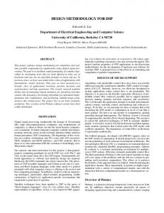
and control physical processes, usually with feedback loops where physical processes affect computations and vice-versa [59]. The application of CPSs in manufacturing determined the born of Cyber-Physical Production Systems (CPPSs) [70] and may lead to the 4th Industrial Revolution, frequently noted as Industry 4.0 [5]. In short, the difference between CPSs and CPPSs is that: CPSs are characterized by flow of information and energy, while CPPSs of information, energy and material. CPPSs work on production lines in which products undergo different manufacturing operations. An example of CPPS is reported in Figure 1.1. This illustrates a production line for filling, straw and shrink plastic application, and palletizing of carton packages. CPSs and CPPSs consist of [10]: • Software-based Controllers (SWs): implement functionality through control software executed by generic hardware; i.e. not tailored for special tasks. SWs have lower computation performance but more flexibility than hardware-based controllers; e.g. microcontrollers. • Hardware-based Controllers (HWs): implement functionality through specific task tailored hardware; e.g. ICs. • Physical plant: physical elements and power electronics; • Interface between controllers and physical plant: sensors, actuators, and communication buses and networks. CPSs design may involve HW/SW co-design. Whereas, built-in solutions are generally adopted for CPPSs. Therefore, the work of CPPSs designers involved in the cyber domain is to develop control algorithms and communication protocols, and to select specific physical means. Control algorithms consist of: • Control logic: generally described in terms of state machines and utilized for performing high-level functionality: controlling system nominal and exceptional behavior, implement Human Machine Interface (HMI) and supervision feedback control systems (e.g. define their set points etc.). • Feedback control systems: generally described in terms of algebraic equations (AEs) and utilized for performing low-level functionality: commanding actuators and sampling sensors.

1.2 Design challenges

3

Fig. 1.1 Example of CPPS: a Tetra Pak production line.

1.2

Design challenges

Design of CPPSs is challenging due to: • Multidisciplinary composition: design integrates a wide variety of heterogeneous disciplines, including control engineering, mechanics, thermodynamics, sensors, electronics, networking, and software engineering [48] [56]. The definition of methodologies and tools for achieving multi-domain co-design is challenging [97] [95] [50] [18]. • Market requirements: from one hand complexity is growing because increasing functionality, flexibility and performance are required. From the other hand, low costs and short time-to-market must be achieved. • Supply chain management: design is shifting more and more in the direction of composing ”Intellectual Properties” blocks designed and manufactured from external companies. However, the objective of having a seamlessly chain in order to minimize errors and time-to-market delays is still unaccounted for. Boundaries among companies are often not as clean as needed and design requirements move from one company to the next in nonexecutable and often imprecise forms, thus yielding misinterpretations and consequent design errors [84].

1.3 Related approaches

4

• Uncertainties: CPSs and CPPSs are characterized by elements whose behavior cannot be exactly modeled. Examples of uncertainties in the physical world are friction, chaos, backlash, flexibility etc. Whereas, uncertainties in the cyber world are mainly due to the not determinism of SWs [32] and communication networks [71]. Assuming that currently (and likely always) is impossible to exactly predict the behavior of physical and cyber elements, methods must be identified for providing a satisfactory design also in presence of uncertainties.

1.3

Related approaches

Systems engineering (SE) is an interdisciplinary field of engineering that focuses on how to design and manage complex engineering systems over their lifecycle [83]. SE techniques are used in complex systems spacing from systems of systems, spacecrafts, embedded systems, robotics, software integration, bridge building etc. In literature, there are several publications from different entities about the definition and description of SE concepts and approaches; e.g. INCOSE [44], NASA [86], US Department of Defense [75], Body of Knowledge and Curriculum to Advance Systems Engineering [82], etc. SE approaches define methodologies for lifecycle management of complex systems through the utilization of models. This thesis introduces a methodology for the design lifecycle of CPPSs. Platform-based Design (PBD) [84] will be adopted to CPPSs. PBD promotes: • separation of functionality and implementation; • reuse of existing solutions; • break-down of the design process in arbitrary abstraction layers. These are consolidated concepts in cyber-physical domains. For example, separation of functionality and implementation can be found in [77] [9], design through integration of existing solutions in [91], and break-down of the design process in abstraction layers in [94] [45] [17]. However, abstraction layers have been proposed based on the considered granularity of the designed system leading to application-dependent solutions. The main innovation achieved in this work is to define abstraction layers on the basis of design objectives and modeling assumptions; i.e. mathematical description of the system, solvers utilized for the resolution and assumptions on the reality. Model-based Design and in general Model-based System Engineering (MBSE) [36] promotes the utilization of models for the lifecycle management of complex systems.

1.3 Related approaches

5

Different works have shown potential benefits on the adoption of MBSE [35] [26]. MBSE implies the definition of: • metamodel: which categories of information the framework must contain; • syntax: how the information must be described; • semantics: how syntax must be interpreted. In order to provide syntax and semantics for MBSE, general-purposes modeling languages have been proposed; e.g. Unified Modeling Language (UML) [74], Systems Modeling Language (SysML) [73], Lifecycle Modeling Language [88], etc. For example, SysML-based design (lifecycle) methodologies can be found in [96] [90] [8] [25] [14], along with SysML-based MBSE frameworks [40] [85]. However, the proposed design methodologies and modeling languages were intentionally left ”loose” for embracing as much domains as possible. Design methodologies define workflow of activities without identifying tools for a practical implementation [9] [22]; e.g. simulations etc. Whereas, modeling languages were partially specified with respect to the semantics causing misunderstandings and emergent behaviors [34]. Profiles were introduced for specifying and extending modeling languages; e.g. [79] [52]. However, the purpose of having a unique language for all the disciplines involved in the lifecycle of complex systems remained unaccounted for. Currently, these languages are mainly utilized for conceptual design and for supporting communication among engineers. In fact, they have the ability to informally communicate design concepts among humans. Another approach for the realization of MBSE is the one proposed within AutomationML [30]: homogeneity. In place of having a central model which abstracts the information contained into Domain-Specific Models (DSMs) through a general-purpose language, DSMs are directly interconnected through neutral data formats and standards. Heterogeneity of DSMs is cut through the conversion into standards. However, standards may not share the same semantics and emergent behavior may appear. Throughout this work, we decided to embrace heterogeneity [81]. The idea is to have a coordination language able to deterministically compose heterogeneous DSMs without converting them into either standards or general-purpose modeling languages [57]. Whereas, nondeterminism is explicitly and judiciously introduced where needed. The contribution of this thesis on the MBSE side is to define a metamodel for implementing libraries of functional and existing elements.

1.4 Thesis outline

1.4

6

Thesis outline

This thesis is targeted to the design of CPPSs. However, the defined concepts may apply to different domains and applications. For this reason, we illustrate the approach through general terms, and then we instantiate it for the design of CPPSs. Modeling and simulations are fundamental tools for the design of complex systems. Chapter 2 introduces the theoretical concepts about modeling and simulation which will be utilized throughout this work. Modeling and simulation need to be utilized within a design methodology in order to bring effective results for the design. Chapter 3 introduces and refines Platform-based Design methodology. Chapter 4 illustrates and sorts the main simulations utilized for CPSs and CPPSs, in order to identify a unique big picture of simulations. Eventually, abstraction layers in which break-down the design process are defined based on the concepts behind the different categories of simulations. Then, the presented tools and approaches are adopted in chapter 5 for the definition of a design methodology for CPPSs. Whereas, modeling patterns for cyber and physical domains are introduced respectively in chapter 6 and chapter 7 in order to apply the proposed methodology to a case study (chapter 8). Eventually, conclusion and future work are reported in chapter 9.

Chapter 2 Modeling and simulation The utilization of models and simulations in the design of complex systems brings tremendous benefits in terms of reducing costs, integrating the involved disciplines, improving quality, and shortening time-to-market [67] [92]. In this chapter, the tools which will be utilized throughout this work are illustrated. Role of modeling and simulation in a design process and their categories and definitions are reported respectively in sec. 2.1 and sec. 2.2. Then, Ptolemy II software and its heterogeneous modeling strategy is introduced in sec. 2.3, along with an implemented modeling tool for reducing model complexity (sec. 2.4). Eventually, an energetic modeling pattern for modeling the dynamic of physical systems is resumed in sec. 2.5.

2.1

Role in the design

Figure 2.1 shows three major parts of the process of designing systems: modeling, design, and simulation. Modeling is the process of gaining a deeper understanding of a system through imitation. Models are abstractions and simplifications of the reality and can therefore only show some aspects of a system. Thus, the crucial issue is that models must be sufficiently meaningful regarding to the actual situation and appropriate use case [44]. Design is the structured creation of artifacts (such as software components) to implement specific functionality. It specifies how a system will accomplish the desired functionality. Simulation shows how models behave in a particular environment. Simulation is a form of design analysis: its goal is to lend insight into the properties of the design and to enable virtual testing. In its most general form, analysis is the process of gaining a deeper understanding of a system through dissection, or partitioning into smaller, more readily analyzed pieces.

2.2 Categories and definitions

8

It specifies why a system does what it does (or fails to do) what a model says it should do. As suggested in Figure 2.1, the three parts of the design process overlap, and the process iterates between them. Normally, the design process begins with modeling, where the goal is to understand the problem and to develop solution strategies.

Fig. 2.1 Iterative process of modeling, design, and simulation [81].

2.2

Categories and definitions

To be effective, models must be reasonably faithful, but they also must be understandable and analyzable. Models are expressed in some modeling language: syntax. Then, in order to be understandable and analyzable, syntax must be associated with a clear and unambiguous meaning: semantics. For example, SysML emphasizes how model diagrams are rendered (their visual syntax), and leaves many details open about what diagrams mean and how models operate (their semantics). Different SysML tools may provide different behaviors to the same diagram. A single SysML model may represent multiple designs, and the behavior of the model may depend on the tool used to interpret the model. Two basic properties for models will be utilized throughout this work. These are: • Determinism: same inputs always correspond to same outputs. Same results are obtained with different runs of simulations, when same inputs are provided to the model within each run;

2.2 Categories and definitions

9

• Predictability: model is able to predict the behavior of the real system with acceptable errors. Deterministic models are not necessarily predictable. In fact, determinism is a property of the model itself, while predictability is a property of the model with respect to the reality. Models can be classified on the basis of different properties. Classifications utilized within this work are based on: • Timing properties: – Untimed models: modeled system either does not change in time or the knowledge of the exact instant in which changes happen is not important for the considered design objectives. Examples for this category are: steady-state analyses, CAD models, functional designs in which time is not considered because an implementation has not been chosen yet, etc. – Timed models: model how system evolves in time. • Modeled technique: – Black box models: models are identified based on the response of real systems (seen as a black box) to standard inputs. Identification techniques are utilized in this case [87] [64]; – White box models: models are identified considering the properties of the constituting systems. Models are generally represented in a mathematical form. Model resolution (simulation) describes the behavior of the system in response to inputs once constants, parameters and initial conditions have been specified. As behavior, we mean the trajectory of the system variables. The whole trajectory of a variable is generally called signal. Two resolution methods can be utilized for models described in a mathematical form: • Analytic approaches: model is expressed in terms of AEs and an exact solution, if exists, is identified. Analytic approaches can be used in steady-state analyses for dimensioning mechanical means, analytic analyses for production systems [41], etc. • Simulation approaches: an exact mathematical solution exists but is too complex for being identified. Numerical techniques are utilized for computing an approximate solution [24]. In this case, system is modeled through sets of differential equations.

2.3 Ptolemy II

2.3

10

Ptolemy II

CPPSs are heterogeneous: heterogeneous models are necessary for simulating their behavior. In fact, each model typically represents only one aspect of the entire system, and thus only part of its total behavior. To evaluate the behavior of the system as a whole, these models must be composed in some fashion so that their properties can be considered together. This heterogeneous composition must represent interaction and communication between models while preserving the properties of each individual model. Brute-force composition of heterogeneous models may result in emergent behavior. Model behavior is emergent if it is caused by the interaction between characteristics of different formal models, and if it was not intended or foreseen by the author of the model. Emergent behavior is therefore always a surprise to the designer, and potentially violates properties the designer expects from the individual formal models, thereby interfering with the ability to analyze the entire model. Throughout this work, we decided to compose models through the hierarchical heterogeneous approach presented in [34]. This approach is studied in the Ptolemy project and implemented within the Ptolemy II software environment. Using hierarchy, one can effectively divide a complex model into a tree of nested submodels, which are at each level composed to form a network of interacting components. The approach constrains each of these networks to be locally homogeneous, while allowing different interaction mechanisms to be specified at different levels in the hierarchy. One key concept of hierarchical heterogeneity is that the interaction specified for a specific local network of components covers the flow of data as well as the flow of control between them. Such a framework is called a Model of Computation (MoC), as it defines how computation takes place among a structure of computational components, effectively giving a semantics to such a structure. To facilitate hierarchical composition, an MoC must be compositional in the sense that it not only aggregates a network of components, but also turns that network itself into a component that in turn may be aggregated with other models, possibly under a different MoC. Interface Automata [29] is used within Ptolemy II to study the compatibility and compositionality of components with their MoC frameworks. Because each local submodel is governed by one well-defined MoC, it can be understood solely in the terms of that MoC, and it can be analyzed in the formal framework defined by it, while at the next higher level of the hierarchy the submodel is considered atomic for the purpose of understanding or analyzing its containing model. This localization

2.3 Ptolemy II

11

of analyzability allows individual components to be refined into more detailed models without affecting the properties of the rest of the system. Ptolemy II modeling approach is based on actors: concurrent components that communicate by exchanging tokens. An actor has a set of input ports, output ports and state. In contrast with other actor-oriented approaches [46] [6], a director / Model of Computation (MoC), rather than the individual actors themselves, defines details of scheduling and communication. This is possible because every actor implements a standard executable interface: an interface constituted of methods which are invoked by the director. The computation of an actor is performed through the calling of its fire method. Typically this method involves reading inputs, processing data and producing outputs. Ptolemy II hierarchical approach is shown in Figure 2.2.

Fig. 2.2 A hierarchical model in Ptolemy II. Next, MoCs which will be used throughout this work are introduced. A deeper description can be found in [81]. These are: • Dataflow (DF) [61]: when an actor is fired, it consumes an arbitrary number of tokens from each input port and produces an arbitrary number of tokens to each output port. Actors are connected and communicate over unbounded FIFO queues. Two types of DF can be simulated: (1) Synchronous DF: actors produce and consume a fixed number of tokens on each firing; (2) Dynamic DF: actors can produce and consume a varying number of tokens on each firing. A valuable property of synchronous DF models is that deadlock can be verified and capacity of buffer can be statically designed. Dataflow domains mostly ignore time, although synchronous DF is capable of modeling streams with uniformly spaced time between iterations. • Continuous time (CT) [63]: model ordinary differential equations (ODEs) and differential algebraic equations (DAEs). The execution of a CT model involves the computation of a numerical solver [24]. In an iteration of a CT model, time

2.3 Ptolemy II

12

is advanced by a certain amount, and a fixed-point value of all the continuous functions is computed. • Discrete event (DE) [55]: actors communicate through events placed on a (continuous) time line. Events are particularly tokens which carry a time stamp, along with a value. Actors process events in chronological order. The output events produced by an actor are required to be no earlier in time than the input events that were consumed. The execution of this model uses a global event queue. When an actor generates an output event, the event is placed in the queue and sorted according to its time stamp. During each iteration of a DE model, the events with the smallest time stamp are removed from the global event queue, and their destination actor is computed. • Synchronous Reactive (SR) [31]: designed for modeling systems that involve synchronicity: applications where things are happening at once (concurrently). SR can be viewed as describing logically timed systems. In such systems, time proceeds as a sequence of discrete steps, called reactions or ticks. Although the steps are ordered, there is not necessarily a notion of ”time delay” between steps like there is in discrete time systems; and there is no a priori notion of real time. Thus, time in this domain is referred as logical time rather than discrete time. • Process Network (PN) [80]: actors are modeled as thread: concurrent processes that communicate through shared variables. On a multicore machine, two threads may execute in parallel on separate cores. On a single core, the instructions of each thread are arbitrarily interleaved. Eventually, two ”modeling patterns” can be implemented in Ptolemy II within the described MoCs [58]: • Finite State Machine (FSM): a state machine is a system whose outputs depend not only on the current inputs, but also on the current state of the system. The state of a system is defined as its condition at a particular point in time. State is represented by a state variable s ∈ Σ, where Σ is the set of all possible states for the system. A FSM is a state machine where Σ is a finite set. In a FSM, system behavior is modeled as a set of states and the rules that govern transitions among them. States have no refinements; • Modal Model: explicit representation of a finite set of behaviors (or modes) and the rules that govern transitions between them. The rules are captured by a FSM

2.4 Aspect-oriented modeling

13

whose states are refined with the implemented system behavior. An example is shown in Figure 2.3.

Fig. 2.3 Example of modal model with two modes.

2.4

Aspect-oriented modeling

Models which implement different heterogeneous aspects of CPSs/CPPSs can become awkward increasing time necessary for the modeling activity; as shown in [7]. AspectOrientation is utilized within Ptolemy II for keeping models simple. Whereas, ObjectOrientation is implemented for populating libraries of reusable actors. A model can be annotated with additional information that is orthogonal to the model. An example would be the evaluation of the cost for implementing a certain system. By annotating each model element with a price, the cost of the entire system can be statically computed. Aspect-Oriented (AO) modeling enables the annotation of actors with information that is evaluated dynamically. Ptolemy II provides two types of aspects [7]: • Communication aspect: wrap the communication between actors by intercepting token transmission. The communication aspect operates on the token from the

2.5 Modeling energetic domains: Power-Oriented Graphs

14

sending actor (e.g. delays, modifies, drops the token etc.) before the receiving actor gets the token. • Execution aspect: wrap the execution of an actor; i.e. the aspect behavior is executed before the actor fire method is called. An example of communication aspect is shown in Figure 2.4. This aspect models the latency introduced by a serial communication. The communication between ActorA and ActorB is annotated with the aspect and configured with parameters describing the latency on that connection. The link will be annotated with a textual parameter that binds the communication link to the SerialCommunication aspect. This aspect may also be associated to other connections in the model. It assumes that a physical wire is utilized for each connection. If networks must be modeled, composite aspects which implement arbitrary models of protocols and network elements should be utilized.

Fig. 2.4 Communication aspect for modeling latency due to serial communication.

2.5

Modeling energetic domains: Power-Oriented Graphs

Bond Graphs [51], port-Hamiltonian approaches [42], Power-Oriented Graphs (POG) [99] and Energetic Macroscopic Representation [19] are graphical modeling techniques


15

which use an energetic approach for modeling physical systems. POG block schemes are easy to use and to understand, and can be directly implemented in dynamic simulators; e.g. Simulink, Ptolemy II, etc. For these reasons, POG technique can be a useful tool for promoting the use of energetic approaches also between beginners and young researchers, and we decided to adopt it throughout this work.

2.5.1

Basic blocks

POG uses power and energy variables as basic concepts for modeling energetic domains. In fact, dissipative energetic domains are characterized by the following properties: • systems always store and/or dissipate energy; • dynamic models describe how energy moves among elements of a system; • energy moves from point to point by means of two power variables. POG uses the two basic blocks represented in Figure 2.5 for modeling energetic domains: 1. Elaboration blocks: model all the elements that store and/or dissipate energy; e.g. springs, masses, dampers, resistances, etc. These are called physical elements (PEs). 2. Connection blocks: model all the elements that ”transform power without losses”; e.g. neutral elements such as gear reductions, transformers, etc. These are called connection elements (CEs). Basic blocks are interfaced through power sections; dashed lines in Figure 2.5. Arbitrary vectors of power variables can be selected within power sections. However, inner product < x, y >= xT y is constraint to model power flowing throughout the section.

2.5.2

Physical elements

POG basic concepts for dynamic modeling are: • Energetic domains: main energetic domains encountered in modeling physical systems are: electrical, mechanical (translational and rotational) and hydraulic. Each energetic domain has its own couple of power variables; • Power variables: divided in:


16

Fig. 2.5 POG basic blocks: a) elaboration block; b) connection block. – Across-variables: variables whose value is determined by measuring a difference of the values at two extreme points of an element; i.e. voltage, linear velocity, angular velocity and pressure; – Through-variables: variables transmitted through an element; i.e. current, force, torque and volume flow rate. • Types of PEs: each energetic domain is characterized by three types of PEs: – 2 dynamic elements (De and Df ): store energy; e.g. capacitors, inductors, masses, springs etc.; – 1 static element (R): dissipates (or generates) energy; e.g. resistors, frictions, etc.; System dynamics can be described by means of four variables: – 2 state variables (qe and qf ): variables which quantify the energy stored within each dynamic element; – 2 power variables (ve and vf ): describe how energy moves among dynamic/static elements. Dynamic/static elements and state/power variables for the main energetic domains are represented in Table 2.1. • Mathematical description of PEs: dynamic element De is characterized by: 1. a state variable qe (t); i.e. internal energy variable;


17

2. a through input variable vf (t); 3. an across output variable ve (t); 4. a constitutive relation qe = Φe (ve (t)) which links state variable qe (t) to output variable ve (t); 5. a differential equation q˙e (t) = Φf (vf (t)) which links state variable qe (t) to input variable vf (t); Energy Ee stored within dynamic element De is function only of the state variable qe : Z Z t

Ee =

0

qe

ve (t)vf (t)dt =

0

Φ−1 e (qe )dqe = Ee (qe )

(2.1)

Dynamic element Df has a ”dual” structure with respect to the structure of dynamic element De . The dual structure can be easily obtained with the following substitutions: qe (t) → qf (t), vf (t) ↔ ve (t) and Φe (ve (t)) ↔ Φf (vf (t)). Static element R is characterized by static function ve = ΦR (vf ) which links input variable vf to output variable ve . POG representation of the types of PEs is reported in Figure 2.6. An example of PEs is next provided for the electrical domain. Considering that power variables are voltage V and current I, and that state variables are charge q and magnetic flux Φ, we have: • De = Capacitor: – Constitutive relationship: q = C ·V ;

(2.2)

dV ; dt

(2.3)

– State differential equation: I =C – Stored energy: U=

Z t

V Idt =

0

Z q 0

q 1 q2 1 dq = = CV 2 C 2C 2

(2.4)

• Df = Inductor: – Constitutive relationship: Φ = L · I;

(2.5)


18

– State differential equation: V =L

dI ; dt

(2.6)

– Stored energy: U=

Z t

V Idt =

0

Z Φ 0

Φ 1 Φ2 1 2 dΦ = = LI L 2 L 2

(2.7)

• R = Resistor: characterized just by static constitutive relationship: V = R · I.

(2.8)

Same relationships can be identified for the other main energetic domains. Whereas, thermal domain has few particularities: power variables are thermal flux Q˙ and temperature variation ∆T , while state variables are heat Q and temperature T . This domain is constituted just by one dynamic and static element: • D = T hermal Capacitor: – Constitutive relationship: Q = m · cp · ∆T ;

(2.9)

d∆T Q˙ = m · cp · ; dt

(2.10)

– State differential equation:

– Stored energy: U=

Z t 0

˙ = Qdt

Z ∆T 0

m · cp d∆T =

Z Q 0

dQ = Q = m · cp · ∆T ;

(2.11)

• R = T hermalResistance: static constitutive relationship: Q˙ = k · ∆T ;

2.5.3

(2.12)

System modeling: composition of PEs and CEs

PEs shown in sec. 2.5.2 interact with the external world by means of two terminals, each one characterized by two power variables ve1 , vf 1 and ve2 , vf 2 .


19

Electrical

Mech. Translation

Mech. Rotation

Hydraulic

De

Capacitor

Mass

Inertia

Hydr. Capacitor

qe

Charge

Momentum

ve (accross)

Voltage

Velocity

Df

Inductor

Lin. Spring

qf

Flux

Displacement

vf (through)

Current

Force

Torque

R

Resistor

Friction

Ang. Friction

Ang. Momentum Ang. Velocity Torsional Spring Ang. Displacement

Volume Pressure Hydr. Inductor Hydr. Flux Volume flow rate Hydr. Resistor

Table 2.1 Main energetic domains: physical elements De , Df and R; energy variables qe , qf ; power variables ve , vf .

Fig. 2.6 POG representation of PEs: dynamic elements De and Df , and static element R. By choosing ve = ve1 −ve2 and vf = vf 1 = vf 2 as new power variables, it follows that power interaction of a PE with the external world can be described by using power section shown in left part of Figure 2.7. The value of power P flowing throughout the


20

section is the product of the two power variables ve (t) and vf (t): P (t) = ve (t) · vf (t)

(2.13)

Dynamic model of each PE can always be graphically described by using block diagrams shown in the right part of Figure 4. These diagrams correspond to the two possible orientations of the corresponding element: vf as input and ve as output, and ve as input and vf as output. Function f (·) in Figure 2.7 symbolically represents one of the dynamic or static models shown in Figure 2.6. If the PE is a static element, both diagrams are suitable for describing element mathematical model. If the PE is a dynamic element, the two diagrams represent the two possible causality modes (integral and derivative) of the dynamic element. Integral causality is physically realizable and useful in dynamic simulation. Whereas, derivative causality is still a correct mathematical model, but not physically realizable and not useful in dynamic simulation. PEs can be connected in: • Series: the terminals of the two PEs share the same through-variable: vf = vf 1 = vf 2 ; • Parallel: the terminals of the two PEs share the same across-variable: ve = ve1 = ve2 ; Summation elements of POG block diagrams (e.g. the circle in Figure 2.5a where • indicates the minus sign) are the mathematical description of Kirchhoff’s Law applied to the across-variables in the closed path of PEs connected in series. Whereas, Kirchhoff’s Law is applied to the through-variables in PEs connected in parallel. Eventually, PEs can also be connected through CEs which redistributes power without neither storing nor dissipating energy; e.g. any type of gear reduction, mechanical levers, electrical transformers, etc. Basic property satisfied by CEs is: P1 = ve1 vf 1 = ve2 vf 2 = P2 Input power flow P1 is always equal to output power flow P2 . A simple example of POG model is shown in Figure 2.8 where a C-parallel PE is connected with an R-series PE. Note the direct correspondence between the power sections 1, 2, 3 in the system and the dashed power sections 1, 2, 3 in the POG scheme. A more complex example with also CEs is shown in sec. 2.5.4.


21

Fig. 2.7 The two POG block diagrams used for graphically describe the mathematical model of the considered PE. Two different orientations correspond to the integral and derivative causality models.

Fig. 2.8 POG modeling of an electrical RC circuit.

2.5.4

Application example and POG graphical rules

A DC motor connected with a hydraulic pump is shown in Figure 2.9. This system involves three energetic domains: electrical, mechanical and hydraulic. The corresponding POG graphical representation in shown in Figure 2.10. As consequence of POG application, power sections presented in the POG scheme have a direct correspondence with the real physical sections. Eventually, the following graphical rules can be derived: 1. All the loops of a POG scheme contains an ”odd” number of minus signs. This rule is a direct consequence of the fact that in the POG schemes a loop always


22

appears when two PEs are connected. Moreover, this loop contains at least one ”minus sign” for letting flowing power have the same positive direction; 2. Chosen two generic points A and B of a POG scheme, all the paths that go from A to B contain either an ”odd” number or an ”even” number of minus signs. This rule follows directly from rule 1; 3. The direction of the power flowing through a section is positive if an ”even” number of minus signs is present along one of the paths which goes from the input to the output of the section. For example in power section 7 of Figure 2.10, power flows from left to right because the red dashed path that goes from B to A contains ”zero” minus signs; i.e. an even number. Same result is obtained considering the left part of section 7: power flows from left to right because the blue dashed path that goes from A to B contains ”one” minus sign; i.e. an odd number. Other formal properties can be derived from POG description, as state-space representation of the system. However, these are not interesting in the context of the presented work; interested readers see [99].

Fig. 2.9 A DC motor connected with an hydraulic pump.


Fig. 2.10 POG scheme of the DC motor with hydraulic pump of Figure 2.9.

23

Chapter 3 Platform-based Design and metamodel for resources Platform-based Design [84] is a methodology widely adopted for the design of CPSs. We strongly believe that CPPSs design, but every design in general, can embrace PBD concepts. This chapter illustrates PBD approach and refines it by introducing a metamodel for characterizing both functional and implementation resources of the arbitrary abstraction layers in which a design process is broken-down. PBD basic definitions and design process are described respectively in sec. 3.1 and sec. 3.2. Then, the introduced categories of resources are populated with elements of cyber-physical and production domains, while the proposed metamodel is illustrated in sec. 3.4. Eventually, an example of its application to production domain is reported in sec. 3.5.

3.1

Basic definitions

The fundamental concept of PBD is the separation of functionality and implementation. PBD provides the following definitions: • Library: contains resources that can be assembled to build a platform. PBD defines two types of resources; i.e. computational and communication. However, we think that other resources must be introduced for completing the picture. Therefore, the following resources can be identified considering that resources interact by exchanging items in terms of information, energy and material [76]: – Computational: utilize received items for performing functionality;

3.1 Basic definitions

25

– Communication: implement the flow of items among resources; – Buffer: store items decoupling computation/dissipative resources; – Dissipative: discharge items; – Connection: convert flowing items. Sec. 3.3 will show how domain-specific elements and their connections fit into this picture. It is important to keep these resources well separated in the library as different methods may be used for modeling and design. For example, different MoCs can be utilized for modeling their behavior. PBD identifies two types of library: – Functional library: also called functional space, defined as the set of functional (implementation independent) resources. Functional resources describe the required functionality. – Implementation library: also called implementation space, defined as the set of available implementation resources. PBD defines as implementation resource an implementation in general: a resource utilized for performing a functionality, not necessarily a physical component; e.g. an algorithm for solving an optimization problem. • Properties: all the elements which are used for abstracting resources. Properties consist in functionality, ”quantities” and interface. Deeper definitions will be provided in sec. 3.4. • Platform: set of resources that are selected from the library and connected together. • Architecture: platform whose Degrees of Freedom (DoFs) have been configured; also called platform instance. • Separation of concerns: design is performed by mapping functionality (what the system is supposed to do) with implementations (how the system does what is supposed to do). It is fundamental to keep functionality and implementation separated. • Common semantics of functionality and implementation: functionality and implementation must share a common semantics for manually or preferably automatically selecting feasible resources. As it will be shown throughout this work,

3.2 Design methodology

26

a common semantics is obtained if the fields of the properties of a functional resource are the same or a subset of the implementation resources that can implement that functionality; • Behavioral models: utilized for calculating properties and can be divided in: – Functional models: model the behavior of a functional platform: a platform built with functional resources. Functional models are utilized for calculating target properties. These can be defined as functional properties. – Implementation models: model the behavior of an implementation platform: a platform built with implementation resources. Implementation models are utilized for configuring an implementation architecture whose properties fulfill the identified functional properties. • Meet-in-the-middle process: PBD is neither a fully top-down nor a fully bottomup approach in the traditional sense; rather, it is a ”meet-in-the-middle” process because it can be seen as the combination of two efforts: – Top-down: select an implementation starting from desired functionality; – Bottom-up: fulfill functionality by building an implementation which consists of already existing resources. The ”middle” is represented by the common semantics in which functionality meets implementation. Figure 3.1 illustrates the meet-in-the-middle concept.

3.2

Design methodology

A design methodology is indicated as the activities which bring from a set of requirements to a product whose properties fulfill target requirements. PBD advocates to break-down the design process in different layers of abstraction. Then, the workflow illustrated in Figure 3.2 can be applied for each layer: 1. Requirements definition: analysis of the design problem and definition of the requirements the designed solution must fulfill. Requirements must be written in a rigorous form for avoiding misunderstandings and for being able to guarantee their verification. This phase includes consistency verification of requirements for assuring that a solution able to fulfill all the requirements can exist.


27

Fig. 3.1 PBD: meet-in-the-middle design. 2. Functional design: also referred as conceptual design. It consists in the conversion of requirements into functionality the system must perform. A functional platform is built by composing functional resources. Then, a functional architecture is configured by identifying functional properties for each resource. This process is performed based on application-dependent methods applied through the use of functional behavioral models. 3. Mapping: (1) selection of implementation resources for building a platform and (2) definition of their parameters for configuring an implementation architecture. Selected resources must fulfill the identified functional properties. Synthesis, optimization, and simulation-based design-space exploration methods can be applied through implementation behavioral models. For example, [38] proposes an optimizer in which a discrete platform selection engine is placed in a loop with a continuous sizing engine. 4. Virtual verification: verification that the designed implementation architecture fulfills target requirements. In CPPSs domain, it generally consists in a verification through simulation models and formal methods. 5. Deployment: physical generation of the solution. Deployment consists in the translation into DSMs of the designed implementation architecture. Model-Driven Development (MDD) [68] is desirable for speeding up and automating the process.


28

6. Physical verification: verification that the properties of the designed implementation architecture fulfills target requirements. Before physically testing the whole solution, incremental hybrid tests can be performed through Hardware in the Loop simulation. Here, real controllers are interfaced with a virtual model of the physical plant. This method is largely utilized in aerospace [33], automotive [49] and manufacturing domain [37] [78]. The illustrated workflow appears linear and sequential, however different iterations may be necessary before a satisfactory solution is identified. Moreover, some activities may be skipped within certain abstraction layers, as will be shown in chapter 5.

Fig. 3.2 PBD process. Not all the implementation resources in the library must be pre-existing components. Some resources may be ”place-holders” to indicate the flexibility of customizing a part of the design that is offered to the designer. Place-holders indicate ideal implementation resources that allocated in an architecture of existing resources make the solution fulfill target requirements. Then, each place-holder becomes the requirements for the following layer of abstraction. The process is iterated until all the functionality are implemented with available implementation resources. Figure 3.3 illustrates the ”fractal nature” of the PBD process in which the same workflow can be applied to each abstraction layer.

3.3 Domains and types of resources

29

Fig. 3.3 Fractal nature of PBD.

3.3

Domains and types of resources

In this section, energetic domains introduced in sec. 2.5.2 are enriched with production and software domains generating a complete picture for CPPSs. Then, physical meanings are provided to the types of resources of each domain. What we called PE is sec. 2.5.2 is here defined as a resource in general. In fact, elements are not necessarily physical. Resources interact by exchanging items in terms of information, energy and material. We define as production domain, the domain in which resources exchange material. Whereas as software domain, the domain in which resources exchange information. As it will be shown in chapter 4, production domain represents an abstract view of assemblies constituted of energetic resources. The following subdivision can be defined based on the exchanged items: • Physical domains: domains involved in physical plants; – Production domain: exchange material; – Energetic domains: exchange energy. These can be: ∗ Electrical domain: exchange electrical energy; ∗ Mechanical Translation domain: exchange linear mechanical energy; ∗ Mechanical Rotation domain: exchange rotational mechanical energy;

3.3 Domains and types of resources

30

∗ Hydraulic domain: exchange hydraulic energy; ∗ Thermal domain: exchange thermal energy; • Cyber domains: domains involved in controllers for physical plants; – Software domain: exchange information; – Electrical domain: exchange electrical energy; also called hardware domain within this context. Electrical domain can be considered both a physical and cyber domain. For example, this domain may be used for generating heat (physical context), for processing electrical signals (cyber context), etc. Different types of resources were identified in sec. 3.1. Next, the illustrated domains are fitted into the defined types of resources: • Production domain: – Computational: machines perform manufacturing operations on inlet material items (products); – Buffer: queues decouple machines and dissipative resources. For example, if a machine fails, downstream machines can still produce as long as queues have products; – Dissipative: products out of acceptable bounds are wasted. • Software domain: – Computational: processes perform functionality on the basis of the implemented control algorithms and received information items; – Buffer: memories decouple the direct communication of information among processes; – Dissipative: all the operations concerning the waste of information; e.g. clear memory area, clear a corrupted information received from a failed resource, etc. • Energetic domain: – Computational: utilize received energy for performing functionality; e.g. inertia for moving a robot arm, capacitors for charging a battery, etc.

3.4 The proposed metamodel

31

– Buffer: decouple computational resources; i.e. inductors and springs; – Dissipative: dissipate energy; i.e. resistors and frictions. Thermal domain has only one dynamic element: thermal capacitor. However, this can be considered both a computational and buffer resource on the basis of the context. For example, a building may use solar panels for heating functionality. The building (thermal capacity) can be considered as a computational resource since accumulate thermal energy for reaching a target temperature. Solar panels warm water and this operation ”decouples” the direct utilization (from the building) of solar energy. Eventually, heat flux exits the building by means of thermal resistances. Therefore, resistances dissipate thermal heat in the context of warming the building. Table 3.1 resumes the identified domains and types of resources. Eventually, communication resources are used for converting flowing items. For example, analog to digital converter, converts analog electrical energy into digital electrical energy, back emf converts electrical energy into rotational mechanical energy (torque) within a DC motor, etc. As final remark, we can say that the extension of the well known energetic domains to software and production domains is just qualitative. In this context, the extension is used for ordering information within the libraries necessary for PBD implementation. However, systems consist of assemblies of resources coming from different domains. As mathematical relationships were identified for modeling the dynamic of resources of energetic domains, quantitative relationships may be found for production and software domain. This may provide a global mathematical model of systems that may facilitate tools which nowadays are computational expensive; e.g. model checking. We invite people expert in software and production domains to investigate whether ”constitutive relationships” can be identified for resources of the defined domains, as happened for energetic domains.

3.4

The proposed metamodel

Based on our academic and industrial experience and supervisioned by SangiovanniVincentelli (the ”father” of PBD), we developed the metamodel for resources illustrated in Figure 3.4. Both functional and implementation resources can be characterized by: • Functionality; • Quantities: defined as the ”numbers” through which resources are abstracted. Quantities can be:

Memory Inductor Lin. Spring Rot. Spring Hydr. Inductor

Process Capacitor Mass Inertia Hydr. Capacitor

Software

Electrical

Translation

Rotation

Hydraulic

Therm. Resistor

Hydr. Resistor

Rot. Friction

Lin. Friction

Resistor

Dissipative Discharge material Discharge information

Table 3.1 Resources for application domain.

Therm. Capacitor

Queue

Machine

Production

Thermal

Buffer

Computation

Domain

Electrical Energy Lin. Mechanical Energy Rot. Mechanical Energy Hydraulic Energy Thermal Energy

Information

Material

Communication

3.4 The proposed metamodel 32


33

– Constants: this category includes either constant functions (e.g. physical space occupied by a machine) or piecewise constant functions of the configured parameters and current operational modes (e.g. for a manufacture machine, energy consumption on the basis of the selected operational mode). – Parameters: numbers that can be configured but are constant functions during resource functioning; e.g. number of processors in a modular embedded architecture; – Operational modes: an operational mode is defined as a discrete number that can assume only one value at a time among the elements of a finite set; e.g. sport or economy modes for a car. – Variables: continuous numbers which vary during resource functioning and are function of all the former categories. Variables generally indicate resource outputs and can be calculated through behavioral models. • Interface: indicates the interface with other resources and the operating environment; e.g. mechanical and electrical connections, supported products for manufacturing machines, etc. • Behavioral model: describes the behavior of the resource in response to inputs once constants, parameters and initial conditions (both states and operational modes) have been specified. Behavioral models can be expressed as: – Look-up tables: resource behavior is described through discrete points mapped in tables. – Mathematical equations: resource is described in a mathematical form and its behavior is obtained by solving the mathematical problem. • Domain-Specific Models: all the models and documents associated with the resource that are necessary for its physical realization. Examples for this category are BOMs, CAD drawings, wiring diagrams, control software, manuals, etc. This metamodel can be used for both functional and implementation resources. In fact, properties for functional resources describe the desired functionality, while for implementation resources the fulfilled functionality. The only exception is constituted by DSMs which apply only for implementation resources. However, this makes sense! In fact, in a perfect world, DSMs should not exist and once configured the implementation architecture, all the DSMs should be automatically generated through MDD. However, we are far from this situation and DSMs need to be associated with implementation


34

resources and defined as much as possible in a modular ”plug-and-play” form. In this way, the number of necessary manual operations is limited. Eventually, we introduce a notation for better characterizing quantities and behavioral models. We define as c1 and c2 the two types of constants, p the parameters, m the operational modes, y the outputs (variables), u and x respectively the resource inputs and states, and m0 , x0 and t0 the initial conditions of modes, states and time. Moreover, u(·) represents the trace of all the resource inputs (i.e. signal), while m(t) the operational mode at time t. The syntax indicates a vector for each category. For example, x indicates the vector of all the states of the resource. The following relationships formally describe quantities: c1 = K 1 ; c2 (t) = K2 (p(t), m(t), t0 ); p(t) = K3 (ti ), i = 1, 2, . . . n; x(t) = f1 (u(·), m(·), c1 , c2 (·), p(·), x0 , t0 ) m(t) = f2 (u(·), x(·), c1 , c2 (·), p(·), m0 , t0 ); y(t) = f3 (u(t), x(t), m(t), c1 , c2 (t), p(t), t0 ); where K1 indicates a constant vectors, K2 (p(t), m(t), t0 ) a vector of piecewise constant functions of the current parameters and operational modes, and K3 (ti ) a piecewise constant function which varies on the basis of the resource configuration; i indicates the i-th resource configuration. The behavioral model is constituted by vectors f1 , f2 and f3 . These vectors depends on the application and the modeled abstraction.

Fig. 3.4 SysML representation of the proposed metamodel.

3.5 Metamodel application to production domain

3.5

35

Metamodel application to production domain

The metamodel proposed in sec. 3.4 is applied for characterizing production domain. In this section, just properties are identified, since possible behavioral models will be shown in the application example (chapter 8). Next, the resulting picture is shown. Computational resources are defined as machines which perform manufacturing operations on products. Machines are aggregations of stations. Their properties are: • Functionality: performed manufacturing operation; • Quantities: – Number of stations: stations within the machine; – Capacity: number of stations multiplied for the number of products processed for station; – Cycle time: time necessary for performing the manufacturing operation; – Production rate: ratio between capacity and cycle time. Production rate is a piecewise constant function of the resource operational mode; e.g. economy, maximum performance, etc.; – Cost: divided in fixed costs (e.g. footprint, installation etc.) and variable costs (e.g. energy consumption etc.). Variable costs are piecewise constant functions of the operational mode, while fixed costs are either constants or parameters function of the selected configuration. – Footprint: required physical space and is either a constant or parameter; – Precision: precision on the performed operation. This quantity provides an indication about the number of waste products and is generally represented with a probability function of the coordinator operational mode. – Utilization rate: percentage of time the machine is correctly working. This quantity is a variable determined through a behavioral model. – Mean Time between Failure (MTBF): for the reason that each operational mode ”stresses” the machine in a different way, this quantity is generally a piecewise constant function of the operational mode; – Mean Time to Repair (MTTR): parameter which is function of the type of failure. – Operational modes: machines may have multiple modes of operations. Modal models are utilized for explicitly representing a finite set of behaviors (or modes) and the rules that govern transitions between them. Transitions are triggered from self-detecting events or from machine supervisor.

3.5 Metamodel application to production domain

36

• Interface: characteristics of the manufactured products. The same quantities and interface can be defined for other resources. The only difference is the performed functionality. Communication resources include both humans and automatic means as robots, conveyors, AGV, etc. These allow the flow of products, and their functionality description must include characteristics of the transported products, implemented communication type (1-to-1 or 1-to-many) and communication protocol. Their production rate is defined in terms of travel time and capacity; i.e. number of transported products for travel. Buffer resources decouple computation/dissipative resources by storing products and must be defined with a service protocol; e.g. FIFO, LIFO, etc. Buffers are shifting from pure passive elements towards smart ones. For smart, we mean that the resource has sensors, actuators and control algorithms. Therefore, the same properties identified for computation resources apply for buffer ones. Dissipative resources discharge not-acceptable products. Therefore, their functionality must include a description of the detected product failures.

Chapter 4 Simulations and abstraction layers for PBD In this chapter, typical simulations for CPSs and CPPSs are introduced sorted in two orthogonal directions (sec. 4.1 and sec. 4.2), and then merged for generating a big picture of simulations available for design and verification (sec. 4.3). Eventually, a subdivision of possible abstraction layers in which brake-down the PBD process is proposed (sec. 4.4).

4.1

Simulations: cyber classification

When SWs are utilized for deploying control algorithms designed through models, different ”horizontal” simulations (representing different degrees of deployment) can be performed for the same ”vertical” modeling abstraction of the physical plant; vertical abstractions will be introduced in sec. 4.2. Whereas, HWs are deterministic and their effects can be modeled as computations with constant delays and different degrees of deployment are not necessary. SWs have computation means which compute algorithms written in processes assigned statically or dynamically to them. Processes can be periodic or event-based, and are computed based on scheduling algorithms and assigned priorities. An operating system is in between control algorithms (written and assigned to processes by users) and computation means [89] [23]. A model of the hardware architecture (e.g. cores, memories, buses, etc.) must be implemented in order to predict execution time for computing processes. However, it is still complex to realize deterministic models able to predict the behavior of real

4.1 Simulations: cyber classification

38

controllers [32]. Our choice is to: utilize less performant but deterministic strategies for configuring SWs, and to model qualitative hardware architectures in order to reach predictable simulations. These concepts will be explained in sec. 6.2. Because of these choices, controller behavior can be predicted and assumptions verified through measurements performed on physical tests [98]. The following deployment layers can be identified for simulating the interaction between SW and physical plant: • Algorithm in the Loop (AIL) [33]: SW ”infrastructure” is neglected; e.g. processes, scheduling, etc. ”Flat” control algorithms are computed with untimed MoCs (SR/DF) when triggered by physical plant; • Software in the loop (SIL) [43]: SW is modeled and control algorithms assigned to processes. The defined models are co-simulated with a model of the physical plant. Three abstractions of SIL can be implemented [13]: – Functional SIL: SW is assumed with ideal behavior: processes are computed periodically without considering scheduling strategies and execution time. Processes are described through modal models solved with DE and whose states are refined with AEs solved with SR/DF. This simulation is utilized for discretizing control algorithms defined within AIL; – Implementation SIL: SW takes time but cannot fail: computation is always performed within the established deadline. In this simulation, processes are assigned to different cores which implement scheduling strategies. Protocols for reading and writing shared memory areas can be investigated in order to avoid race conditions, along with scheduling strategies. This is possible through the utilization of PN for modeling concurrent execution, and AO for implementing scheduling strategies; – Deployment SIL: SW takes time and can fail: computation can terminate after the established deadline. Random delays which model SW execution time are introduced within the implementation SIL model. System response to failures is designed. • Hardware in the Loop (HIL) [65]: real SW is connected to a virtual model of the physical plant which is synchronized to the controller. Actual SW execution time on the basis of the computed process and controller state can be obtained through measurements. Simulation time is synchronized to real-time in Ptolemy II by setting to true the parameter synchronizeToRealTime of the top-level director.

4.2 Simulations: physical plant classification

39

• Physical test: both plant and controller are real.

4.2

Simulations: physical plant classification

Simulations can also be classified ”vertically” on the basis of the modeling abstraction of the physical plant: mathematical description of the system and MoC(s) utilized for the resolution [54] [94]. A list is reported below sorted for levels of abstraction. The simulation categories are illustrated with typical use cases: • Dataflow Simulation: system is modeled through AEs solved neglecting the concept of time. DF are utilized for modeling the flows of items. A resource executes when its required data inputs become available. This simulation is used in the production domain for qualitatively configuring an architecture. • Discrete Event Simulation (DES): system is modeled through AEs and probabilistic equations solved with DE. DESs are used for modeling production domain when time is considered. • Dynamic Simulation (DS): system is modeled through ODEs and constraints (e.g. rotational joints etc.) resulting in a set of DAEs. CT is used for the resolution. DSs are utilized for modeling energetic domains. Two abstractions can be defined: – Kinematic Simulation (KmS): DAEs are based on kinematic attributes; e.g. velocity, acceleration, etc. KmSs are mainly utilized for the definition of control logic and definition of kinematic properties for energetic resources [47]. – Kinetic Simulation (KS): DAEs are based on kinetic attributes; e.g. force, mass, etc. KSs are used for different purposes as dimensioning type and size of actuators, design feedback control systems, etc. • Hybrid simulation (HS): models solved with CT are co-simulated with models solved with DE. HSs are used for modeling energetic resources with multiple modes of operations. Modal models computed with DE are utilized for explicitly representing a finite set of behaviors (or modes) and the rules that govern transitions between them. States of the modal models are refined through equations solved with CT; e.g. physical collisions [60]. • Geometric Simulation (GS): system is modeled through continuity equations described as a set of partial differential equations (PDEs). Both stationary and

4.2 Simulations: physical plant classification

40

transient behaviors can be investigated. These simulations are used for problems where geometry plays an important role as structural analysis, magnetic fields, heat transfer, turbulent flow, etc. For example, in [53] GS is used for determining stress-strain of components and machines during static and dynamic conditions. Other MoCs have been introduced which can be considered as particular implementation of the illustrated ones. For example, PTIDES [100] for DE, CyPhySim [21] for CT, etc. For a complete list see last publications of Edward Lee research group1 . However, each MoC is particularly suited for specific formal analyses. For the reason that formal analyses are neglected within this work, we decided to include just the presented and more general MoCs. Future work may enlarge the proposed picture assigning the most suited MoCs to each abstraction layer and design phase. Table 4.1 resumes vertical abstractions of simulations including all the analytic analyses which can be performed during a design process. Analyses are not simulations. Since analyses are based on the resolution of AEs, an exact analytic solution (if exists) is identified and not an approximation. Untimed simulations are used for functional designs: functions are designed independently from implementation. Therefore, the concept of time is not considered in this phase. DESs are used for the analysis of systems in which constituted elements do not exchange energy. This results in event-based algebraic and probabilistic models. Steady-state analyses and simulations are ”symbolically” placed under the resolution through CT, even if time independent (for asymptotically stable systems) or periodic equations (for simply stable systems) are solved. In fact, stable systems are characterized by transient behaviors followed by steady-state ones. At steady-state, time dependent equations of the transient behavior turns into time independent or periodic equations. When transient behaviors are negligible, steady-state analyses are utilized for dimensioning mechanical means based on their steady-state dynamic properties. For example, given upstream and downstream pressure (p1 and p2 ), fluid (ρ) and valve type (cd ), Bernoulli equation can be used for identifying valve necessary area (A) given the target flow rate (V˙ ): q

V˙ = cd A

2 ρ (p2 − p1 )

1 http://ptolemy.eecs.berkeley.edu/publications/index.htm

4.3 Simulations: big picture

41

DSs are utilized for identifying steady-state and dynamic properties which are function just of the time. Whereas, steady-state and dynamic GSs are used respectively for modeling steady-state and dynamic properties which are function of the geometry; e.g. velocity profile in a fluid moving with turbulent flow. Structural analyses are finalized to the design and verification of structural properties of physical bodies; e.g. calculation of maximum deformation in the sections of a loaded F ·L3 cantilever qbeam (δ = 3E·I ), identification of natural frequencies of a cantilever beam K E·L (f = 2πL m ), etc. Structural static and dynamic GSs are used for modeling structural properties on physical bodies, when algebraic relationships cannot be identified. The difference between DSs and dynamic GSs is the numerical solver utilized for the resolution [24]. DSs are described through differential equations which are function of the time. Time is discretized in the resolution and numerical solvers for ODEs and DAEs are utilized; e.g. Runge-Kutta, Euler, etc. Dynamic GSs are described through differential equations which are function of time and space. Both time and space are discretized in the resolution and finite element or finite volume solvers are utilized depending on the application. Whereas, static and steady-state GSs are described through differential equations which are function just of space. Therefore, space is discretized in the resolution.

4.3

Simulations: big picture

The simulations defined in sec. 4.1 and sec. 4.2 are merged for generating the big picture represented in Figure 4.1. As said before, this picture is not definitive and in future may be enlarged. The picture is identified considering that the interaction between cyber and physical domain occurs within the MoC utilized for the resolution of the physical domain. The X in the figure indicates a deployment layer not useful based on the utilized MoC and solvers. For example, untimed simulation has no concept of time, so it is not worth to use it for SIL and HIL simulations; whereas in GS, the effects of SW are abstracted through the utilization of variable forces. The ˜ indicates that the corresponding deployment simulation can be performed with approximations. For example, a CT model can be connected either to a DE simulator that implements the model of SWs (SIL) or to real controllers (HIL). The interaction is based on rendezvous communication points as happens in the Functional Mock-up

/

Time and Spatial PDEs /

/

Structural static simulation Structural dynamic simulation

/

/

/

Structural analysis

Structural

Table 4.1 Categories of analyses and simulations based on physical plant modeling abstractions.

/

Steady-state geometric simulation Dynamic geometric simulation

Hybrid simulation

/

Spatial PDEs

/

/

Continuous time Steady-state analysis Kinematic simulation Kinetic simulation

/

Discrete event Discrete event simulation

/

Dataflow simulation

AEs

Kinematic DAEs Kinetic DAEs AEs + DAEs

Untimed

Equations

4.3 Simulations: big picture 42

4.3 Simulations: big picture

43

Interface for co-simulation [69]. However, just constant communication steps are currently supported [20] [93]. Cyber and physical domains are able to interact but with different timing with respect to the real interaction. However, if communication time step is shorter than the solver time step of the physical plant model, interaction happens with the proper timing. Eventually, AIL simulation indicates control algorithms computed through SR. We assume that CT and DE solvers are able to compute through SR, as happens for example in Stateflow within MATLAB/Simulink.

Fig. 4.1 Simulations for cyber-physical and production domains.

4.4 Domains and layers for PBD

4.4

44

Domains and layers for PBD

In this section, we propose categories for grouping the arbitrary abstraction layers in which a design process is broken-down. This subdivision is based on design objectives for physical plant and modeling assumptions. Modeling assumptions consists in: items exchanged among resources, utilized mathematical description and MoCs for the resolution, and assumptions on the reality. The name of each category is given by the domains considered while modeling the physical plant. The following domains can be identified: • Production domain: physical resources exchange information and material, and are modeled as black boxes without considering the dynamic of the constituting elements, resulting in a DE mathematical description. Physical design objective is to identify Key Performance Indicators (KPIs) of resources [11]; e.g. cycle time, MTBF, MTTR, etc. • Energetic domain: physical resources exchange information, energy and material, and are modeled as white boxes considering the dynamic of the constituting elements, resulting in a CT mathematical description. Physical design objective is to identify kinetic quantities of resources; e.g. bandwidth for sensors, maximum torque for motors, etc. • Structural domain: physical resources exchange energy and are modeled through continuity PDEs in order to analyze their structural aspects. Physical design objective is to identify structural quantities of physical resources; e.g. Young’s modulus. Then, production and energetic domains can be broken-down in the same abstractions identified within horizontal layers: • Functional layers: resources are modeled with ideal behavior: functionality is designed neglecting the concept of time;; • Implementation layers: resources are modeled with nominal behavior: time for performing functionality is included but failures do not occur; • Deployment layers: failures may occur. These categories are defined based on our experience on CPPSs, but we think that the definitions are general and applicable to different domains. We invite other domains to test this subdivision, and to refine and correct it whether necessary. Within each

4.4 Domains and layers for PBD

45

category, arbitrary horizontal layers can be used on the basis of the application as shown in Figure 4.2; each mapping symbol indicates a horizontal layer.

Fig. 4.2 Categories for horizontal layers and resulting PBD process.

Chapter 5 Platform-based Design: application to CPPSs In this chapter, the picture of simulations reported in sec. 4.3, and the domains and layers illustrated in sec. 4.4 are targeted to the design of CPPSs. PBD phases are populated with starting information, and with simulations for achieving target information. Structural domain is considered a mechanical-specific phase that only marginally integrates physical and cyber domains. For this reason, we do not include structural aspects within this work. However, future work may consist in populating horizontal layers for this domain; e.g. including design of structural frames, bearings for mechanical shafts, identification of natural frequencies of flexible bodies, etc. Different behavioral models can be implemented within energetic domain. For example, filling operations may have behavioral models based on the combination of DSs (e.g. for regulating valves etc.) and computational fluid dynamics (CFD) simulations. For example, CFD (dynamic GS) can be used for modeling liquid behavior, if turbulent flows must be investigated. While illustrating the methodology, we consider a design in which dynamic GSs are not necessary. In the proposed design process, arbitrary horizontal layers were placed within the categories identified in sec. 4.4. As said before, the farther layers are considered, the more DoFs must be configured: design-space is enlarged but optimization and prediction becomes difficult. The choice of in which layers break-down the design process is arbitrary. After having performed the qualitative application example shown in chapter 8, we decided to breakdown the defined layers into physical and cyber design. However, this subdivision

47 is theoretical and further layers are likely necessary during a real design, in order to reduce configurable DoFs for each layer. The choice must be performed in accordance with design methods and tools available for the design. Physical design is meant to design physical domains; i.e. production and energetic. Whereas, already built solutions are assumed for controllers in the design of CPPSs. Therefore, cyber design consists in the design of control algorithms and communication protocols, and selection of specific physical means. During the illustration of the approach, we use three abstractions for the selection of implementation resources. We define the selection of: • Feasible resources: selection of resources based on ideal quantities; i.e. quantities identified considering ideal assumptions. • Qualitative resources: selection of resources based on nominal quantities; i.e. quantities identified considering implementation non-idealities. • Specific means: selection of specific physical means based on real quantities; i.e. quantities identified considering deployment non-idealities. For example, feasible resources may be the selection of using Programmable Logic Controllers (PLCs), and qualitative resources the choice of using PLCs with partial quantities; e.g. number of cores, capacity of memories, etc. Whereas, specific means consist in the selection of specific PLCs; e.g. Rockwell MicroLogix 1400. CPPSs are characterized by different modes of operations [2]; e.g. cleaning, maintenance, production, etc. Each mode is generally refined by a state machine that model the different operational states within the considered mode; e.g. initialization, failure, etc. Each state of the mode state machine is refined with control algorithms; i.e. control logic and feedback control systems. The resulting architecture is a hierarchy of modal models for each smart resource. States of the highest modal model are called operational modes. Then, each operational mode is refined with a modal model whose states are called operational states. Eventually, operational states are refined with control algorithms. The chapter is structured in this way: sec. 5.1 defines the design activities within production domain, while sec. 5.2 the ones within energetic domain. Eventually, considerations from authors are reported in sec. 5.3.

5.1 Production domain

5.1

48

Production domain

The overall design process starts with the definition of stakeholder requirements. These express properties required to the system, and the operational environment in which must operate. Within the whole production domain, cyber resources are assumed with ideal behavior: do not take time and cannot fail. Within this layer, cyber design is performed before physical design. In fact, operational modes and states must first be defined and then quantities of resources are identified for each mode and state. The abstraction layers and design phases illustrated in Figure 5.1 are utilized for the design of production and cyber domains: • Functional layers: physical resources are assumed with ideal behavior: do not take time and cannot fail. – Cyber design: discrete event simulation is utilized. 1. Requirements definition: operational modes must be identified. 2. Functional design: FSMs are developed for defining operational modes of resources and their coordinator. Moreover, coordinator-resources interface variables and protocols are established for managing transitions of operational modes. 3. Mapping: already implemented FSMs for operational modes can be adapted and reused. 4. Virtual verification; – Physical design: dataflow simulation is utilized. 1. Requirements definition: a physical functional architecture must be defined and ideal quantities be configured. 2. Functional design: required functionality is identified and assigned to physical resources which are sorted in a functional architecture: computational resources are sorted and communication protocols configured when shared resources are utilized. Ideal quantities of these resources are configured. 3. Mapping: feasible physical resources are selected. 4. Virtual verification; • Implementation layers: physical resources take time but cannot fail. Discrete event simulation is utilized for both physical and cyber design.


49

– Cyber design: 1. Requirements definition: nominal operational states must be identified. 2. Functional design: FSMs defined within cyber functional layer are converted into modal models. A FSM refines each operational mode. Nominal operational states and transitions are identified; i.e. without considering failures and recovering after failure states. Moreover, coordinator-resources interface variables and protocols are established for managing transitions within nominal operational states, and for communicating quantities of resources to coordinator. 3. Mapping: already implemented FSMs for nominal operational states can be adapted and reused. 4. Virtual verification; – Physical design: 1. Requirements definition: implementation non-idealities are configured and ideal quantities are refined. Constant and piecewise constant quantities of the operational modes and states are identified; 2. Functional design: dataflow models are converted into discrete event models by introducing time for performing functionality. Execution time and capacity is configured for computation and communication resources, while maximum capacity of buffers is identified. 3. Mapping: qualitative resources are selected; 4. Virtual verification; • Deployment layers: physical resources are assumed with real behavior: failures can occur. – Cyber design: discrete event simulation is utilized. 1. Requirements definition: all the operational states must be identified. 2. Functional design: nominal operational states of each operational mode are refined by including failures. For example, resources may fail and states for repairing and recovering after failures are introduced. Moreover, coordinator-resources interface variables and protocols are established for managing transitions within all operational states, and for communicating failure quantities of resources to coordinator; e.g. a failure variable may indicate the resource type of failure.

5.2 Energetic domain

50

3. Mapping: already implemented FSMs for nominal and failure operational states can be adapted and reused. 4. Virtual verification; – Physical design: discrete event simulation and analytic approaches [41] are utilized; e.g. fault tree analyses. 1. Requirements definition: specific means must be selected. 2. Functional design: deployment non-idealities (MTBF and MTTR) are configured and nominal quantities are adapted for facing failures of resources. Moreover, precision quantity is introduced in order to simulate failures on the resource performed functionality. Dissipative resources must be inserted for wasting faulty products; 3. Mapping: specific means are selected and configured in order to fulfill functional properties. 4. Virtual verification; The information for deploying the solution is now available. Deployment is done by generating necessary DSMs. HMI is also designed. Then, physical verification is executed. Discrete event HIL is utilized for verifying the fulfillment of target quantities and bounds of controllers, and the correctness of control logic. Eventually, physical tests are performed for verifying that the overall solution fulfills stakeholder requirements.

5.2

Energetic domain

These layers are utilized for the design of energetic and cyber domains. Here, physical design is performed before cyber design. Properties of place-holder production resources are translated into stakeholder requirements for this domain. The abstraction layers and design phases illustrated in Figure 5.2 can be identified within energetic domain: • Functional layers: ideal behavior is considered. For energetic domain, ideal behavior is defined as the kinematic behavior. Whereas, cyber resources do not take time and flat control logic is computed. – Physical design: kinematic AIL simulation is utilized.


51

1. Requirements definition: a physical functional architecture must be defined. 2. Functional design: a functional (kinematic) architecture is built and a physical type is defined for each resource. Geometric and kinematic quantities are identified; e.g. position in the working space, kinematic trajectories for actuators, etc. Eventually, control logic is developed for all the operational states of each operational mode. 3. Mapping: feasible physical resources are selected. 4. Virtual verification; – Cyber design: UML/SysML diagrams are utilized. 1. Requirements definition: a cyber functional architecture must be configured. 2. Functional design: defined control logic is divided into cyber functional groups. 3. Mapping: past functional groups decomposition can be adapted and reused. 4. Virtual verification; • Implementation layers: implementation behavior is considered. For energetic domain, implementation behavior is defined as the kinetic behavior. Whereas, cyber resources take time but cannot fail: computation is always performed within the established deadline. – Physical design: hybrid functional SIL simulation. 1. Requirements definition: kinematic properties of resources and trajectories identified in the functional layers must be implemented. 2. Functional design: kinetic properties of actuators (e.g. inertia etc.) are identified and geometric properties are refined. Feedback control systems are designed for implementing the defined kinematic trajectories. Transmission must be designed, whether necessary, and acceptable bounds must be defined for physical uncertainties; e.g. backlash, friction, etc. 3. Mapping: qualitative physical means are selected. 4. Virtual verification;


52

– Cyber design: hybrid functional and implementation SIL simulations are utilized. 1. Requirements definition: implementation properties of cyber resources must be identified; 2. Functional design: the choice of using SW/HW for functional cyber groups is performed. In the event of HW, higher bounds for the computation of control algorithms deployed in HWs are identified. Whereas for SW, cyber functional groups are assigned to periodic and event-based processes, while feedback control systems are discretized. Period is identified for both periodic processes and feedback control systems. Period definition provides also the bandwidth required to sensors. These activities are performed through hybrid functional SIL simulation. Then, hybrid implementation SIL simulation is used for qualitatively configuring controllers: processes are assigned to different cores which implement scheduling strategies. Protocols for reading and writing shared memory areas can be investigated in order to avoid race conditions, along with scheduling strategies of processes. Eventually, capacity and higher bounds for transport time are identified for communication resources. 3. Mapping: qualitative resources are selected. 4. Virtual verification; • Deployment layers: deployment behavior is considered. Both physical and cyber resources can fail. – Physical design: discrete event simulation and analytic approaches are utilized. 1. Requirements definition: specific means for resources must be selected. 2. Functional design: production place-holder failure quantities are brokendown to the designed resources; 3. Mapping: specific means are selected; 4. Virtual verification; – Cyber design: hybrid deployment SIL is utilized. 1. Requirements definition: specific means for resources must be selected. 2. Functional design: parameters for random functions modeling execution and communication time are identified. Dissipative resources/functionality

5.3 Discussion

53 are introduced for wasting corrupted information; i.e. information written after the established deadline.

3. Mapping: specific means are selected; 4. Virtual verification; The information for deploying the solution is now available. Deployment and physical verification is performed as within the production domain. The only difference is that hybrid HIL simulation is utilized for physical verification phase.

5.3

Discussion

This chapter has illustrated a PBD process for CPPSs formalizing functional models before the selection of implementations. However, many DoFs must be configured for defining quantities before the selection of specific physical means. The problem is complex and nowadays specific means are mainly selected for physical and cyber resources without the former identification of target values through functional models. Then, physical tests are performed for verifying the fulfillment of target requirements. Engineering and optimization methodologies must be introduced for each identified design phase. In Figure 5.1 and Figure 5.2, we use production domain for designing a production line, and energetic domain for a machine. However, this does not mean that production domain is only used for line configuration, and energetic domain for machine configuration. In fact, machine configuration may involve both production domain and energetic domain as will be shown in the application example (chapter 8). Abstraction layers must be identified based on the design objectives and MoCs utilized for the resolution of behavioral models, and not on the considered granularity of the designed system.

5.3 Discussion

54

Fig. 5.1 PBD for CPPSs: production domain.

5.3 Discussion

55

Fig. 5.2 PBD for CPPSs: energetic domain.

Chapter 6 Modeling patterns for cyber design Cyber design is implemented by simulating control algorithms with a model of the physical plant. Cyber design consists in the definition of control algorithms and in their deployment into HWs/SWs. In this chapter, simulation deployment abstractions identified in sec. 4.1 are utilized for supporting cyber design. In particular, cyber design is decomposed in the layers identified in sec. 4.4 and modeling patterns are introduced for utilizing the identified simulations. As said before, control algorithms consists of control logic and feedback control systems. Both can be deployed into HWs/SWs. However, when SWs are used, feedback control systems are assigned only to periodic processes, while control logic can be assigned both to periodic and event-based processes.

6.1

Functional layers

In this phase, control algorithms are designed considering ideal behavior: time and failures are neglected. AIL simulation is utilized for designing functionality of control algorithms. Untimed MoCs compute control algorithms interacting with a model of the physical plant. Moreover, defined control logic is divided into cyber functional groups. Cyber functional groups must be formed considering that each group will be deployed either in a HW or as a process within a SW. Cyber functional groups can be represented as UML/SysML class/blocks and reported in a class/block definition diagram.

6.2 Implementation layers

6.2

57

Implementation layers

In this phase, time is included. The following activities are performed: 1. Assign cyber functional groups to HWs/SWs: each group will be deployed in either HWs or as a process within a SW; 2. HWs design: higher bounds for the computation of cyber functional groups deployed in HWs are identified; 3. SWs design: two phases can be identified: • Discretization: cyber functional groups are assigned to periodic and eventbased processes, while feedback control systems are discretized generatic difference equations and assigned to periodic processes. Eventually, period for periodic processes is identified; • Implementation: qualitative quantities of SWs are designed: processes are assigned to different cores which implement scheduling strategies. Protocols for reading and writing shared memory areas can be investigated in order to avoid race conditions, along with scheduling strategies of processes. Functional and implementation SIL simulations are utilized for performing these activities. HWs are deterministic and in both simulations can modeled as untimed computation with a constant computation delay. Whereas, different models must be implemented for SWs within functional and implementation SIL simulation. Functional SIL simulation is used for performing discretization phase. SWs can easily be modeled within functional SIL simulation; i.e. through the models of periodic and event-based processes next illustrated. Whereas, implementation is performed through implementation SIL simulation. Here, assumptions and modeling patterns must be introduced for modeling SWs within this simulation abstraction. Next, the utilized modeling patterns and assumptions are illustrated. SWs are devices for computing processes. Two type of strategies can be implemented for periodic processes: • Read-compute-write: every time a process is computed, inputs are read, control algorithm is executed and eventually outputs are written. Writing instant of outputs is function of the execution time taken for computing the process.

6.2 Implementation layers

58

• Write-read-compute: outputs computed the previous period are written, inputs are read and eventually computation is performed. Writing instant of outputs is independent from execution time. Thus, I/O operations are deterministic, given that execution time is less than the period. As said in sec. 4.1, we decided to model software infrastructure of SWs. Whereas, hardware architectures of SWs are modeled just qualitatively; i.e. number of cores, and private and shared memories. We utilize few critical assumptions for modeling SWs. These can be implemented in PLCs making them ”safe devices”: almost completely predictable but less performant than microcontrollers or else. The following assumptions are utilized: 1. Write-read-compute for computing periodic processes; 2. Static assignment of processes to cores: no run-time change of computing core is allowed for processes; 3. Fixed priority scheduling algorithm without preemption: each core schedules processes based on static priorities and without preemption; 4. Event-based and periodic processes are disjoint sets: generally event-based processes manage critical failures and preempt periodic processes. In this case, we assume that event-based processes either are assigned to specific cores/HWs or do not preempt periodic processes. Next, it is shown how a SW which implements the presented assumptions can be simulated through AO modeling. • Periodic processes: the proposed model for a periodic process is shown in Figure 6.1. Process contains the implemented control algorithm and is computed with untimed MoCs. A DiscreteClock triggers the computation by reading Inputs vector. VectorDisassembler extracts all the vector elements, while MostRecent makes the process be computed at the ticks of the DiscreteClock. If Inputs port had been directly connected to the process, a computation would be performed every time an element of Inputs vector changes value. VectorAssembler groups process outputs in a unique vector, while Previous makes process produce the outputs computed the previous period. Eventually, Const updates Outputs vector; • Event-based processes: process is computed when an event is received. Eventbased processes are generally utilized for safety critical functionality. Therefore, Previous actor is not inserted: determinism is lost in favor of reactivity. Proposed model for event-based processes is shown in Figure 6.1;

6.3 Deployment layers

59

• Scheduling algorithm: execution aspects are introduced on the basis of the qualitative hardware configuration. Figure 6.2 illustrates a controller with two processors. Here, processes are statically assigned to CPUs. ProcessA and ProcessB are assigned to CPU1, while ProcessC and ProcessD to CPU2. Every CPU implements a fixed priority scheduling algorithm without preemption through the FixedPriorityScheduler1 execution aspect. Priority is set as parameter of the association of the aspect to actors. PN director is utilized for modeling concurrency of the two CPUs. Parameter placed at top-level hierarchy implements shared memories. The defined aspects model software deployment in a clean way without increasing model complexity. Aspects are reusable and can be employed in different models. Removing aspects from models is done by simply deleting them; no other changes to the model are required. The utilization of aspects for modeling SWs facilitates design-space exploration. In fact, different deployment configurations such as hardware qualitative architectures and scheduling strategies can be quickly modeled and simulated.

6.3

Deployment layers

In this layer, SWs take time and can fail: computations can exceed the defined deadline. Whereas, because of their determinism, HWs cannot fail the computation. Deployment SIL simulation is utilized for identifying an acceptable ”precision” parameter for computation. In order to model computation uncertainties, a random delay actor is placed before the writing of outputs; as shown in Figure 6.3 for a periodic process.

1 FixedPriorityScheduler:

the aspect implements java control logic which can be found

https://chess.eecs.berkeley.edu/ptexternal/src/ptII/doc/codeDoc/ptolemy/actor/ lib/aspect/FixedPriorityScheduler.html at:


Fig. 6.1 Model of periodic and event-based processes.

60


Fig. 6.2 Example of a SW with two cores each one computing four processes.

Fig. 6.3 Deployment model of a periodic process.

61

Chapter 7 Modeling patterns for physical design Physical design is implemented by simulating models of the physical plant with models of the cyber domain. In this chapter, simulation physical abstractions identified in sec. 4.2 are utilized for supporting physical design: both production and energetic domains. In particular, physical design is decomposed in the layers identified in sec. 4.4 and modeling patterns are introduced for utilizing the identified simulations.

7.1 7.1.1

Production domain Functional layers

Dataflow simulation is utilized for designing functionality of resources. Within DF, resources exchange just material (products). Tokens models the exchanged products neglecting the concept of time. In fact, tokens contain just a value and not a time stamp. Composite actors illustrated in Figure 7.1 have been used for building a library of functional resources: • Accumulator: Repeat accumulates an arbitrary number of tokens equal to parameter blockSize. Then, tokens are repeated for a number of times equal to parameter numberOfTimes. By setting blockSize = 1 and numberOf T imes = Nacc , Repeat accumulates Nacc tokens and release them as a stream without repeating. Eventually, DownSample merges inlet stream generating just one output token.


63

• Stations: by setting Nacc = Nstations , Accumulator produces a token when a number of tokens equal to Nstations is accumulated. Then, the produced token triggers MultiInstanceComposite that generates a number of tokens equal to Nstations . Eventually, Commutator creates a unique streams of tokens. Functional library of resources utilized within these layers is represented in Figure 7.2 and consists of: • MachineTransformer: consists just of Stations actor; • MachineAssembler: assembles products. Synchronizer is necessary for constraining all the input ports to have at least one token before being processed. Commutator creates a unique streams of tokens. Eventually, DownSample is used for merging inlet tokens; • MachineDisassembler: disassembles products. MultiInstanceComposite replicates inlet token for the number of times specified by parameter Ndis .

Fig. 7.1 Accumulator and stations DF composite actors.

7.1.2


In this layers, time is included and discrete event simulation is utilized. Within DE, resource exchanges information and material. Events contain a value and a time stamp,


64

Fig. 7.2 Functional library of DF functional physical resources. and model the exchanges information and products. IDEF formalism is proposed for placing interface variables [27]. Composite actors exchange material through the horizontal I/Os, and information through the top I/Os. Composite actors illustrated in Figure 7.3 have been used for building a library of functional resources: • Accumulator: produces an output event after having received an arbitrary number of input events. This composite actor consists just of logical actors: SR director is utilized for the computation; • Stations: Server consists of a queue for modeling the buffer upstream the machine and a timer for modeling machine CycleTime. Capacity output port provides server queue capacity at simulation run-time, while CycleTime is a piecewise constant function of the operational mode settable through an input port. Stations settable parameters are MaxCapacity of server queue and Nstations . Accumulator generates an event when a number of events equal to Nstations is accumulated. Then, event is placed in the Server queue. Every time Server finishes to process an event, it triggers MultiInstanceComposite that generates a number of events equal to Nstations . Eventually, SingleTokenCommutator creates a unique streams of events.


65

Functional library of resources utilized within this layer is represented in Figure 7.4 and consists of: • Buffer: this actor models buffers outside the production line. Whereas, buffers within the production line are called Queues. Source/raw materials are provided as inputs of a line. These contain a fixed number of products. For example, a carton roll contains a certain number of flat carton packages. When triggered, MultiInstanceComposite generates a number of events equal to parameter Nproducts . SingleTokenCommutator converts the generated events into a unique stream of events. Eventually, Queue accumulates events and releases them when an event is received from the Release input port. Capacity output port provides queue capacity at simulation run-time. Queue maximum capacity is set equal to Nproducts ; • Communication: Stations is configured with TransportCapacity and QueueCapacity parameters. TravelTime must be provided through input port and run-time capacity is produced in Capacity output port; • MachineTransformer: as communication but configurable through Nstations and MaxCapacity. CycleTime must be provided through input port and run-time capacity is produced in Capacity output port; • MachineAssembler: Synchronizer is necessary for constraining all the input ports to have at least one event before being processed. Then, Merge actor merges the incoming events. The discardEvents configuration parameter of Merge must be set to true. In this way, inlet events are joint and not converted into a stream of events; • MachineDisassembler: Stations triggers a MultiInstanceComposite which generates an arbitrary number of events equal to Ndis .


Fig. 7.3 Accumulator and stations DE composite actors.

66

Fig. 7.4 Functional library of DE implementation physical resources.

7.1 Production domain 67


7.1.3

68

Deployment layers

Within these layers, resources have failures. A FSM decorates the models of resources defined in sec. 7.1.2 in order to model failures and their fixing. We consider a FSM with four states. However, the choice to neglect or include states is a trade-off about model complexity and influence that the states have in the overall behavior with respect to the DoFs which must be configured. The utilized states are: • Idle: resource is ready for starting working and is waiting for a command from line controller; • Production: resource is working; • Failure: resource is in a failure situation and is being repaired. • Down: resource is not producing because of failures in one or more resources of the line. It is worth to remark that this is only one possible implementation. The critical point for a good design is to choose the proper abstraction on the basis of the application. These states provide the necessary abstraction for our application. In fact, different operational modes (e.g. maximum performance, economy, etc.) and operational states (e.g. starting, execute, etc.) can be implemented with a run-time change of CycleTime / TravelTime parameters. Moreover, within this abstraction layer, all the possible failures are grouped in an averaged value. Therefore, only one state is necessary for modeling failures and not one state for each type of failure. Then, a logical interface must be defined for configuring transitions of resource FSM. The defined logical interface must consists of: • I/Os: role of the information exchanged with line controller; • Syntax: how syntactically information is exchanged; e.g. BOOL, integer, structure, etc.; • Semantics: how syntax must be interpreted. The utilized logical interface is represented in table 7.1. Integer variable Command is used for grouping resource inputs, while integer variable State for grouping resource outputs. Each resource must be characterized with a specific integer value: ResourceID. Then, transitions are configured as shown in Figure 7.5.


69

Interface Input Input Input Input Output Output Output Output Output

Syntax Command=1 Command=2 Command=3 Command=ResourceID State=1 State=2 State=3 State=4 State=5

Semantics ToProduction ToDown ToIdle ToFailure Idle Production Down FailureOccur FailureFixed

Table 7.1 Resource logical interface.

Fig. 7.5 Illustration of resource FSM. Eventually, resources may also fail to perform their functionality. For example, communication resources may make products fall down, machines may manufacture products with characteristics outside the required tolerances, etc. A precision parameter must be added to the description of functional implementation resources. Then, dissipative resources which waste faulty products must be introduced. Precision and IdealDissipativeResource composite actors are shown in Figure 7.6: • Precision: multiports have been used for allowing the utilization of this actor also for MachineDisassembler. Commutator creates a unique streams of tokens from multiple inputs. Bernoulli outputs a boolean value on the basis of the probability set in Precision parameter. An integer is assigned to the introduced fault through ErrorTag parameter. Default makes ErrorTag overwrite the default TRUE token, when Bernoulli produces a TRUE token. Eventually, Distributor converts the stream of tokens into multioutput tokens. Synchronous DF director


70

is utilized because just logical actors are used. In particular, Commutator and Distributor are simulated which are typical of DF domain. • IdealDissipativeResource: Inhibit discharges an inlet event when triggered. CompositeActor contains the logic for triggering Inhibit when an events equal to ErrorTag is received. These composite actors are used for refining implementation resources. Then, deployment library illustrated in Figure 7.7 is built. Each resource is modeled with the ModalModel reported before. Production state contains the implementation resources defined in sec. 8.1.2 followed by Precision actor. Moreover, a NonInterruptibleTimer is triggered every time resource enters within Production state. NonInterruptibleTimer models resource MTBF. In fact, timer progress only when resource is in Production. Production has a history transition for saving timer value when leaving the state. The same is defined for Failure state. NonInterruptibleTimer here models MTTR. Each resource must be configured with MTBF, MTTR, Precision, ResourceID and ErrorTag parameters. Moreover, all the parameters of implementation layer must be filled.


Fig. 7.6 Precision and IdealDissipativeResource DE composite actors.

71

Fig. 7.7 Functional library of DE deployment physical resources.

7.1 Production domain 72


7.2 7.2.1

73

Energetic domain Functional layers

In these layers, ideal behavior is considered. For physical (energetic) resources, ideal behavior is defined as the kinematic behavior. Therefore, kinematic simulation is utilized. Physical resources are geometrically dimensioned through CAD drawings and then placed in the working space through a CAD assembly. A functional geometry is defined since specific means for resources have not been selected yet. For example, a conveyor may be modeled as a parallelepiped block, etc. Footprint specification identified within production domain must be fulfilled. Then, CAD assembly is imported into a kinematic tool and simulated. Unfortunately, Ptolemy II has no libraries for this kind of graphical kinematic simulation. Therefore, we selected the commercial tool industrialPhysics 1 (iP). iP defines the library of kinematic resources shown in sec. 7.8. To be fair, products are called dynamic elements within iP and their motion is computed based on dynamic equations. For example, products react to collisions based on impulse equations. Whereas, all the other elements of the library are purely functional and kinematic. For example, actuators perform kinematic trajectories, grippers grab collided products when a boolean variable is set to true, etc. In order to implement the simulation, user draws the solution in a CAD environment and then import the result within iP as STEP/STL file. After that, a role (library element) is assigned for each resource; i.e. part of the CAD assembly. On the basis of the assigned role, a mathematical model is attributed to the resource, along with functional and kinematic interface variables. Eventually, user fills resource interface variables statically through parameters and dynamically through control logic written within iP. iP provides many other functionality as real-time computation for implementing HIL simulations, automatic PLC code generation from the defined control logic, etc. However, throughout this work, we concentrate only on the functionality that we consider useful during the design. 1 industrialPhysics:

kinamatic AIL simulator produced by Machineering GmbH & Co. KG

http://www.machineering.de


74

Fig. 7.8 Functional library of iP.

7.2.2


In these layers, nominal behavior is considered. For physical resources, nominal behavior is defined as the kinematic behavior. Therefore, kinematic simulation is utilized. POG energetic technique presented in sec. 2.5 is proposed.

7.2.3

Deployment layers

In these layers, failures must be modeled. Analytic analyses as fault tree analyses and DESs are utilized. Failure quantities of the designed place-holder resource is


75

broken-down into failure quantities of the elements which compose the place-holder resource. In the event DEs is utilized, pattern identified in sec. 7.1.3 are adopted.

Chapter 8 Application example In this chapter, the proposed methodology is applied to a case study. The objective is to: • verify the defined layers of abstraction, and starting and target information defined for each layer; • provide examples on how to implement the identified simulations. The definition of rigorous approaches for documenting the design process, and for describing requirements and resources will be matter of future work; the same for the identification of methodologies for functional design and mapping phases, formal methods for virtual verification, and design patterns for deployment through MDD. For these reasons, all the process is documented in a textual-based syntax and is performed in a ”conceptual” form. Requirements are defined without numerical values and models are proposed but not extensively simulated and analyzed. In this application example, we suppose that a stakeholder requires the functionality of the line illustrated in Figure 1.1. However, none line with the required properties is already in a hypothetical company library of past solutions. Therefore, a design activity is necessary. Throughout this chapter, we show the design for production operational modes. However, these phases should be repeated for each operational mode. A list of possible stakeholder requirements is illustrated in Table 8.1. These are a set of functionality, performance and design constraints. The list may be refined considering also interface requirements and implementation details as safety, operational environment, delivery deadline, etc. However, the identified list contains all the information necessary for verifying the proposed approach without getting lost in the

8.1 Line configuration: production domain

77

complexity of a real case study. The implemented example is focused on performance fulfillment and deals only marginally tools and simulations for safety requirements. Requirement Unwind packaging material Sterilize packaging material Apply cap Form package Fill package with liquid Apply straw Sort packages in pattern of 3 Apply shrink plastic on the sorted packages Place 60 packages on each pallet Apply shrink plastic on the pallet Place pallet on stack Production rate MTBF MTTR Waste Products Package characteristics Footprint Cost

Category Functional Functional Functional Functional Functional Functional Functional Functional Functional Functional Functional Performance Performance Performance Performance Constraint Constraint Constraint

Table 8.1 List of stakeholder requirements.

8.1 8.1.1

Line configuration: production domain Functional layers

Cyber design In this phase, FSMs are developed for defining operational modes of machines and their coordinator: line controller. Moreover, line controller-machines interface variables and protocols are established for managing transitions of operational modes. Figure 8.1 illustrates a simulation for defining line controller operational modes. User can interact by setting Input parameter. Arbitrary operational modes can be developed. For example, production can be a hierarchical state with four possible modes: automatic maximum performance, automatic economy, semi-automatic and manual.


78

Fig. 8.1 Definition of line controller operational modes. Physical design Dataflow simulation is utilized for configuring a qualitative physical architecture and identifying ideal quantities of resources. Functional requirements are grouped into functional groups considering Tetra Pak machine subdivision: • Filling machine → unwind and sterilize packaging material, apply caps, form packages and fill them with liquid; • Straw applicator → apply straw; • Sorter → sort packages in pattern; • Shrink applicator → apply shrink plastic on packages; • Palletizer → packages are placed on a pallet and shrink plastic is applied. An architecture is configured connecting functional resources defined before. The result is shown in Figure 8.2. Synchronous DF director is utilized, since each actor consumes and produces a fixed number of tokens. Simulating one iteration / period1 , F iringsP erIteration variable provides the number of times each actor is executed within one period. The simulation termination without errors witnesses that line is configurable; i.e. none deadlock is present. Having 1 In

DF simulation, period is generically called least upper bound.


79

configured an architecture in series, this may be noticed also without simulation. However, in circular architectures (with feedback loops), simulation may help verifying line ”schedulability”. Just one station is inserted for each machine as starting point of the design process. F iringsP erIteration provides the number of times each station is executed for period. For example, modeling one station for machine and simulating one iteration, we obtain that the number of produced products is P roductsF orP eriod = 1; i.e. Display output. StrawApplicator has F iringsP erIteration = 60. In fact, each iteration: NStraws Iteration

=

P allet Iteration

P kgs Straws Straws Straws · PLine allet · Line · P kgs = 1 · 20 · 3 · 1 Iteration = 60 Iteration

Then, CycleTime available for each station can be identified through target production rate Φ: CycleT imeM achineN =

Φ P roductsF orP eriod

3600 s · F iringsP erIterationM achineN

(8.1)

Simulation can be repeated with stations in parallel; i.e. setting Nstations parameter of each machine. Equation 8.1 provides a static relationship between CycleTime and Nstations for each machine. In fact, P roductsF orP eriod and F iringsP erIteration are function of Nstations . Different line configurations can be simulated and ideal values for CycleT ime and Nstations can be identified for each machine. Ideal values represent the best achievable result. Designed solution will have nonidealities and its properties will be more or less close to the identified ideal values. This is the same concept of Carnot cycle2 applied to production domain. A lower bound constraint is sometimes specified for CycleT ime. For example, melting manufacturing operations need time for cooling products. These specifications will constrain the identification of the proper number of stations. DoFs of this layer are resumed in Figure 8.3. If a resource provides products to different resources, arbitrary communication protocols would be implemented through communication aspects. 2 Carnot

cycle provides an upper limit on the efficiency that any classical thermodynamic engine can achieve during the conversion of thermal energy into work, or conversely, the efficiency of a refrigeration system in creating a temperature difference (e.g. refrigeration) by the application of work to the system.


80

Fig. 8.2 Functional line architecture of functional resources.

Fig. 8.3 SysML diagram of the DoFs during functional physical design layer. Discussion Within the presented layers, functional models can be used during the definition of stakeholder requirements. In fact, the illustrated models consist in a schematic and executable form of requirements. Verification of consistency and conceptual communication can be achieved both for physical and cyber domains. Moreover, HMI can be configured together with stakeholders. Whereas, quantitative results provided by DF simulation are used as starting iteration point within following design phases.

8.1.2


Cyber design FSMs defined within cyber functional layer are converted into modal models. A FSM refines each operational mode. Nominal operational states and transitions are identified; i.e. without considering failures and recovering after failure states. Moreover, line controller-machines interface variables and protocols are established for managing transitions within nominal operational states, and for communicating quantities of resources to line controller. Figure 8.4 illustrates a model for designing the FSM of the filling machine production


81

mode. Transitions are triggered from line controller (through Input variable) and machine status (through State variable). For example, machine has finished the initialization operations and can start producing. Quantities are communicated from machine to line controller. For example, Counter is inserted for communicating number of processed products.

Fig. 8.4 Filling machine: nominal operational states of production modes.

8.1 Line configuration: production domain 82


83

Physical design Discrete event simulation is utilized for configuring values of implementation nonidealities and refining ideal quantities identified in sec. 8.1.1. An architecture is configured instantiating functional resources defined above. The result is shown in Figure 8.5. DE director is utilized for model resolution. Output ports of machines are connected to buffers for making buffers release products. In order to simulate the architecture, user must provide cycle time value to the information input port of each machine, and travel time to communication actors. Then, the information output port will provide simulation run-time capacity. DoFs of this layer are resumed in Figure 8.6. Nproducts parameter of buffers is generally a constant that depends on the utilized material and supplier. Therefore, Nproducts can be considered as constant and not as a DoF. Whereas, required maximum capacity of each queue is function of the configured DoFs. If no shared resources are configured, communication protocol is not a DoF. Therefore, the total number of DoFs becomes: h

DoF s = 1·Nmachines +2·Ncommunications = 1·Nmachines +2· (Nmachines − 1) + NBuf f ers (8.2) In the presented case study, there are 5 machines and 6 buffers: 25 DoFs should be configured in order to fulfill target production rate for each operational mode. An ideal value has already been identified for CycleTime and Nstations of each machine. These values will be used as starting point of the design iteration.

Fig. 8.5 Functional line architecture of implementation resources.

i


84

Fig. 8.6 SysML diagram of the DoFs during implementation physical design layer. Discussion Cyber design becomes awkward when performed within Ptolemy II and in general within ”software based on building blocks”. In fact, different hierarchies must be created and coordinated for each resource. However, our objective is to show design phases and necessary MoCs, and not to identify the best tool for each phase. Therefore, Ptolemy II is used for communicating concepts, even if in practice other more specific tools would be used for cyber design within production domain. Engineering theories and optimization methods are necessary for configuring DoFs of physical design. For example, a good practice in industries in to use a V model for defining production rate of machines. The most critical machine is configured with a certain production rate and assumed in the bottom part of an hypothetical V architecture. Whereas, production rate of other machines is configured to 20% more the upstream/downstream machine; respectively upstream for machines on the right side of the V, and downstream for machines on the left side. The application of this heuristic rule would reduce the DoFs concerning production rate of machines to 1 DoF: the production rate of the most critical machine. The objective is to reduce DoFs with engineering theories and heuristic rules, and then optimize the remaining DoFs. A local optimal solution that fulfills stakeholder requirements would be identified. In fact, the identification of a global optimum is too difficult, since too many DoFs must be configured. Some machines may have no upstream queue. For example, this is the case of a conveyor that directly provides products to machine stations. In this case, MaxCapacity parameter of machine server is set to zero. The proposed design layer has 25 DoFs. Therefore, in a practical implementation this layer would likely be broken-down in closer layers. However, this decision must be taken when available design methodologies and tools are defined.


8.1.3

85

Deployment layers

Cyber design Within this layer, resource behavior defined in cyber implementation layer must be refined by adding failures. Nominal operational states of each operational mode are refined by including failures. For example, resources may fail and states for repairing and recovering after failures are introduced. Moreover, coordinator-resources interface variables and protocols are established for managing transitions within all operational states, and for communicating failure quantities of resources to coordinator; e.g. a failure variable may indicate the resource type of failure. The model shown in Figure 8.4 can be utilized also for developing complete resource behavior. Physical design Discrete event simulation is utilized for configuring values of deployment non-idealities and refining nominal quantities identified in sec. 8.1.2. An architecture is configured instantiating functional resources defined above. The result is shown in Figure 8.7. Publisher and Subscriber actors have been inserting for avoiding too long and crossing wires within the model. However, model still becomes difficult to built and manage. Future work may identify modeling patterns for making it manageable. For example, Dissipative and Communication actors may be implemented as communication aspects. Publisher and Subscriber included in the model of each resource, etc. DoFs of this layer are resumed in Figure 8.8. Other deployment non-idealities can be deduced from these DoFs. For example, a conveyor is utilized for implementing a communication resource. Given QueueCapacity, TravelTime and dimensions of the transported products, conveyor length and kinematic properties can be calculated. Then, these quantities together with MTBF, MTTR and Precision are utilized for determining a physical mean and consequently its cost. If cost or footprint are too much, former design phases must be repeated in order to generate a solution which fulfill stakeholder requirements but that required a less performant conveyor. If no shared resources are utilized, the total number of DoFs becomes: DoF s = 4 · Nmachine + 5 · Ncommunication + 3 · Nbuf f er + 3 · Ndissipative

(8.3)


86

This is a huge number of DoFs. However, intermediate layers can be easily simulated. For example, precision can be neglected by setting P recision = 1 for all the resources. Failures can be assumed just for machines by setting M T BF = ∞ for communication, buffer and dissipative resources.

Fig. 8.7 Functional line architecture of deployment resources.

Fig. 8.8 SysML diagram of the DoFs during deployment physical design layer.


87

Discussion As it can be noticed, producing a good solution and not only a working solution is a complex task. From one hand, engineering and optimization methods must be utilized for configuring DoFs. From the other hand, each repetitive operation should be automated in order to let designers concentrate on the challenging problems. Each smart resource has operational modes and operational states, and is commanded and communicates with other resources through a coordinator. Moreover, each mode is characterized with a common high-level behavior; e.g. within each mode, resource performs initialization operations before implementing a functionality, has failures, etc. Packaging Machine Language (PackML) [1] has been introduced in order to standardize: • operational states and transitions for each operational mode; • communication among smart resources coming from different Original Equipment Manufacturers; i.e. though definition of syntax and semantics of interface variables. PackML FSM is reported in Figure 8.9. Unfortunately, weak semantics has been defined and PackML cannot be considered a standard yet. In [12], we tried to define semantics for PackML tools, but much work must be done on this field. In conclusion, PackML goes in the direction of a rigorous and standard approach that may facilitate MDD and communication among smart resources. We hope that scientific community will increase researches in this field, in order to either make PackML become a standard or for introducing more rigorous approaches. The objective must be to have a standard software architecture in which designers fill control algorithms identified through simulation, and then control code is automatically deployed. If all the necessary resources already exist within the company library, solution is ready to be deployed. Whereas, if place-holder production resources have been utilized, a functional analysis must be performed before moving to energetic domain. Placeholder production resources are divided into smart functional groups: assemblies of sensors, actuators and control algorithms. The choice is performed on the basis of the implemented functionality, interaction with other functional groups and characteristics of existing resources in the company library. For example, a filling machine consists of 5 functional groups, which respectively performs the function: ”Unwind packaging material”, ”Sterilize packaging material”, ”Apply cap”, ”Form package” and ”Fill

8.2 Machine configuration: energetic domain

88

package with liquid”. If a place-holder production resource consists of more than one functional groups, another production domain iteration must be implemented for the identified functional groups. Place-holder production resource is considered as the new line controller and the identified functional groups as resources. Production properties, operational modes and operational states are identified for each functional group. This process is iterated until functional groups can no more be refined. Again, it can be noticed that the break-down of a design methodology cannot be performed relying on the considered system granularity but just on the utilized computational tools and design objectives.

Fig. 8.9 PackML state machine.

8.2

Machine configuration: energetic domain

After production domain, a place-holder production resource must be designed through energetic domain. In this section, we suppose there is no existing Sorter machine in the company library of machines that fulfills the identified production properties. Sorter machine cannot be decomposed in functional groups, so energetic domain can start. Moreover, ”neighbor” communication and dissipative resources selected within production domain must be configured.


89

Properties identified for sorter machine becomes stakeholder requirements for energetic domain. Whereas, neighbor upstream and downstream communication and dissipative resources constitute part of the environment in which machine must operate.

8.2.1

Functional layers

Physical design In this layer, ideal behavior is considered. For physical resources, ideal behavior is defined as the kinematic behavior. Whereas, cyber resources do not take time and flat control algorithms are implemented. Kinematic AIL is utilized. An architecture is configured through iterations between CAD environment and iP, until a satisfactory solution is reached. The following properties are identified: • Type of resources: a functionality can be implemented by different physical means. Trade-off analyses are performed for identifying the best solution; • Geometric quantities: these include footprint and position of resources; • Control logic: control logic is developed for all the operational states of each operational mode defined within production domain. In fact, actuators must be coordinated on the basis of the information coming from sensors; • Kinematic quantities: resource production rate identified in the production domain must be fulfilled. Kinematic properties of resources are defined; e.g. velocity of communication resources, kinematic trajectories of actuators, etc. Iterations among CAD environment and iP have been performed. Different physical means have been investigated for sorter machine; e.g. robot which place three products stacked along a wall into a downstream conveyor. Eventually, the solution reported in Figure 8.10 was identified. Two linear actuators block the first product of the pattern, and release it when three products are accumulated. Light barrier sensors are used for detecting products. The utilization of two nonaligned sensors is necessary for detecting fall and attached products. The blue object models pneumatic air for discharging fall products, while the yellow one is a sensor for computing the number of wasted products. Eventually, black object makes products fall down in order to design discharge control logic and kinematic properties of the dissipative resource. A conveyor with guides is utilized for continuously transporting products. Control logic schematized in Figure 8.11 has been defined for sorter machine within execute operational state of production operational mode. Linear actuators implement the kinematic trajectory illustrated in Figure 8.12.


90

Fig. 8.10 Functional architecture of the Sorter machine: screenshot from iP simulation.

Fig. 8.11 Linear actuators: control logic of execute state within production mode. Cyber design Control logic defined in previous design phases is divided in cyber functional groups considering that each group will be deployed either in a HW or as a process within a


91

Fig. 8.12 Forward kinematic trajectory for linear actuators. SW. In this example, we created a functional group for each operational mode of sorter machine. Having performed a qualitative design, this was the only possibility. The defined cyber functional blocks are shown in Figure 8.13.

Fig. 8.13 SysML representation of the defined cyber functional blocks.

Discussion It can be noticed that the outcomes of production domain are broken-down into quantities for this layer. For example, geometric and kinetic quantities of sorter machine must fulfill footprint, cycle time and number of stations specified by production quantities. Eventually, place-holder production resources are implemented with kinematic resources. For example, sorter machine is implemented through two linear actuators and two light sensors.


8.2.2

92


Physical design In this layer, implementation behavior is considered. For physical resources, implementation behavior is defined as the kinetic behavior. Whereas, cyber resources still do not take time and flat control algorithms are implemented. Kinetic AIL is utilized. Within functional layers, types of resources were identified, along with kinetic trajectories for actuators. Given the selected categories of actuators (e.g. electrical motors, pneumatic pistons, etc.), a kinetic model is implemented. Kinetic model must be utilized for configuring kinetic quantities of actuators (e.g. inertia, mass, etc.) and refining geometric quantities; e.g. shaft radius of electrical motors. Moreover, feedback control systems must be designed for fulfilling target kinematic trajectories. This phase must include also the design of transmissions, whether necessary. For example, if a gear box is utilized, gear ratio must be identified. Eventually, kinetic model must define acceptable bounds for physical uncertainties as friction, backlash and flexibility of bodies. POG technique was used for identifying the kinetic model of linear actuators. It consists in a linear implementation of the DC motor shown in Figure 2.10. Then, a continuous regulator is designed and kinetic properties of linear actuators are configured, along with regulator parameters. Continuous regulator means that regulator is computed every time step of physical plant solver. A cascade control of position, velocity and current is implemented as shown in Figure 8.14. In this layer, necessary sensors are identified; i.e. outputs of physical resources. Feedback control systems must be dimensioned in order to have acceptable position errors. Acceptable values of position errors are identified through precision production parameter and considered application. In fact, large position errors determine imprecision in the performed operation. For example, within sorter machine, a position error larger than product width makes actuators miss the first product of the pattern. Therefore, position error and application determine the actual precision value. This must be within the specifications identified within production domain. Next design phases will add non-idealities and downgrade position error. Therefore, a safe margin must be considered when continuous regulators are designed, and iterations with the following design phases may be necessary.

Fig. 8.14 Configuration of quantities of linear actuator and design of continuous regulator.

8.2 Machine configuration: energetic domain 93


94

Cyber design In this layer, hybrid functional and implementation SIL simulations are utilized for configuring implementation non-idealities of cyber resources. Cyber resources take time but cannot fail: computation is always performed within the established deadline. Hybrid SIL simulations are performed interfacing under DE director physical resources computed with CT and models of controllers. Cyber and physical domains exchange variables through ZeroOrderHold and PeriodicSampler actors. First, the defined cyber functional groups and feedback control systems are assigned to HWs/SWs. If HW is utilized, simulation is used for identified higher bounds for computation. Whereas, in the event of SWs, discretization must be implemented. Discretization of feedback control systems deployed in SW is implemented through hybrid functional SIL. Difference equations are identified for continuous regulators, along with necessary period. Numerical methods or direct design can be utilized [39]. Hybrid functional SIL model utilized within the case study is shown in Figure 8.15. LinearActuator is decorated with PeriodicSampler and ZeroOrderHold actors. Whereas, continuous regulator is discretized with difference equations and solved with SR. Then, a period for each periodic process must be defined for cyber functional groups. Period must be identified on the basis of the implemented functionality. For example, control logic for detecting critical failures will be implemented as event-based or fast periodic processes. Whereas, supervision functionality will be implemented in slow periodic processes; e.g. management of transitions among operational modes and communication with HMI. Different tools can be utilized on the basis of the application. Hybrid (kinematic) functional SIL models are created simulating failure scenarios and verifying resulting reactive behavior. Formal methods can also be adopted for this purpose. The definition of the period identifies also a specification for the bandwidth required to sensors. In fact, each sensor must be able to sample at the rate identified from the process to which sensor provides inputs. In conclusion, the selection of period for control logic must be performed on the basis of its functionality concerning safety, whereas for feedback control systems on the basis of target precision; i.e. performance. After that, hybrid implementation SIL simulation is used for qualitatively configuring controllers: processes are assigned to different cores which implement scheduling strategies. Protocols for reading and writing shared memory areas can be investigated in order to avoid race conditions, along with scheduling strategies of processes. Even-


95

tually, capacity and higher bounds for transport time are identified for communication resources. Different controller configuration can be investigated through the modeling pattern identified in sec. 6.2.

Fig. 8.15 Hybrid functional SIL model for discretizing continuous regulator.

Discussion Within this phase, precision identified within production domain guides the design of feedback control systems and their discretization. However, overall precision of the implemented solution will be identified after cyber failures are considered. Within this layers, safety requirements play a fundamental role for the deployment of cyber functional groups. Methods and simulations must be identified for designing solutions which fulfill safety requirements. Eventually, we utilized safe assumptions and modeling patterns for obtaining deterministic and predictable models of SWs. Multiple runs of simulations may be utilized for studying system behavior when more performant and less deterministic choices are implemented.


8.2.3

96

Deployment layers

Physical design In this phase, MTBF and MTTR identified within production domains must be brokendown to the constituting elements; i.e. sensors and actuators. DESs shown in sec. 8.1.3 and analytic approaches are utilized. However, for the reason that the objective of this work is to provide modeling tools and not to define specific methods for the different phases, this activity was not implemented within the case study. Cyber design In this layer, SWs take time and can fail: computation can exceed the defined deadline. Hybrid deployment SIL simulations are utilized for analyzing and designing system behavior when failures occurs. Dissipative resources (functionality) must be implemented for discharging corrupted information; i.e. outputs not computed within the deadline. Eventually, a final value of precision quantity can be obtained on the basis of the selected mean and standard deviation for process computation time (Figure 6.3). This value of mean and standard deviation should guide the selection of specific means for SWs. Discussion PBD process has been qualitative implemented. DoFs of the different abstraction layers have been identified and tools for breaking-down quantities until a satisfactory physical solution is reached, have been provided. However, engineering and optimization methods must now be applied to the provided tools for configuring the identified DoFs.

Chapter 9 Results and conclusions 9.1

Results

Different results have been achieved throughout this work. These can be resumed in: 1. Identification of a big picture of simulations for CPPSs: simulations available for CPPSs design and verification have been introduced and sorted in two orthogonal directions: physical abstraction and cyber deployment; 2. Introduction of a design methodology for CPPSs: PBD design methodology has been applied to CPPSs and broken-down in abstraction layers identified on the basis of the design objectives and MoCs utilized for the resolution of behavioral models; 3. Definition of a metamodel for populating libraries of reusable functional and implementation resources: POG energetic technique for modeling the dynamic of physical systems has been qualitatively extended to production and information domains in order to generate a metamodel for characterizing resources; 4. Definition of modeling patterns: different modeling patterns have been introduced for the application of the approach to a case study. In particular, two results must be underlined: • Utilization of aspect-orientation for modeling software behavior during SIL simulations. • Definition of a Ptolemy II library for modeling functional and implementation architectures of the abstraction layers defined within production domain. Library is not definitive but should be improved in terms of usability, above

9.2 PBD: benefits

98

all within deployment layers. The presented library allows scaling the production design process. This is difficult to obtain with commercial simulators. In fact, they are more suited for modeling all the production properties of resources. For example, dataflow simulation cannot be implemented in commercial discrete event simulators; In conclusion, this work has provided modeling tools, abstraction layers and guidelines for performing a design based on PBD. Now, the provided tools must be refined and associated to design methodologies and rigorous approaches for a practical implementation.

9.2

PBD: benefits

An ideal PBD approach would allow overcoming current design challenges of CPPSs introduced in sec. 1.2. Main benefits due to the utilization of PBD are: • Multi-domain co-design: reasoning in terms of functionality allows abstracting the problem through the identification of a common layer in which multi-domain co-design can be performed. • Complexity and quality: the break-down of the design process into different abstraction layers allow reducing complexity and facilitate the application of computational expensive tools, improving quality of the design; e.g. model checking. • Increase design-space: reasoning in terms of functionality allows considering all the available solutions. For example, in the embedded domain, a functionality can be deployed into SW/HW. If design starts by writing control software, the space of possible solutions is limited. Whereas, reasoning in terms of functionality (control algorithms in the case of embedded systems) allows embracing all the possible solutions and the choice among SW/HW becomes a consequence of trade-off analyses during mapping phase. • Reducing costs and time-to-market: the following activities are promoted: – Reuse: a solution is mainly designed combining existing implementation resources;

9.2 PBD: benefits

99

– Process automation: operations which do not involve ”human factor” can be automated as: ∗ Mapping: analyses can be automated for the selection from the library of feasible resources during design-space exploration. Moreover, synthesis and optimization techniques can be automated for configuring quantities of the selected resources. ∗ Implementation: patterns and model transformations can be automated through the adoption of MDD paradigm. – Continuous verification: it is well known that the cost due to errors increase exponentially with the phases of the design lifecycle. Therefore, design process must allow continuous verification in order to have early detection of errors [18] [28]. This is the reason why most of the traditional design processes as waterfall and V model turned to be inefficient. In fact, verification is performed just in the final part of the design. PBD enhances continuous verification through the virtual and physical verification phases. In fact, fulfillment of requirements must be verified before moving to the following abstraction layer. • Uncertainties: uncertainties of implementation resources can be considered as DoFs in the functional design phase. Acceptable bounds are identified and then feasible implementations are selected. • Company organization: – Design methodology: companies are forced to structure the design process identifying necessary layers, methodologies and tools. – MBSE: PBD enforces the identification of a virtual framework for tracing the design process and documenting past solutions. The definition of libraries make know-how accessible without relying anymore just on few experienced designers. – Supply chain management: separation among functionality and implementation, along with the utilization of different abstraction layers provide a structured framework for assigning boundaries among the companies involved in the supply chain. Moreover, the utilization of rigorous approaches for the description of requirements and resources reduces misunderstandings and integration errors.

9.3 PBD: utilization concerns

9.3

100

PBD: utilization concerns

Before the adoption of PBD, the following decisions must be taken: 1. Horizontal layers: identification of precisely defined abstraction layers in which mapping process takes place. For precise definition of abstraction layers, we mean the definition of: • vertical boundaries: starting and target information for each layer; • horizontal boundaries: boundaries among resources during the composition of an architecture; i.e. which functions are assigned to each specific resource and how resources interface with each others; • methodologies and tools for each design phase. This decision is complex and application-dependent. Having ”far” layers enlarges design-space but makes prediction and optimization difficult. As it was shown in the application example (sec. 8), an indicator about the space among two layers may be provided by the number of DoFs of the functional behavioral model. 2. Populate the libraries: this involves the choice of which resources worth having in the libraries. Cost and time for bringing a resource into a library and for its maintenance is generally larger than its design. In fact, the process involves: • Functionality: assure correct functionality in different environments; • Quantities: define variation range for parameters and operational modes, and the corresponding values of constants; • Interface: define resource interface and how flexible should be; • Behavioral model: identify a model able to predict, with acceptable errors, resource behavior. This operation includes model validation through the comparison with experimental data obtained testing the resource; • Domain-Specific Models: identify which DSMs are necessary for the deployment and define them as much as possible in a modular plug-and-play form; whether MDD transformations are not available. 3. Grammar: agreement on syntax and semantics for representing all the phases of the design process and for describing functional and implementation resources.

9.4 PBD for CPPSs: future work

101

4. Security: the definition of libraries of past and market solutions would make know-how accessible to anyone in the company. Accession protocols must be identified. These critical decisions are application-dependent and should be agreed with the top design management level. As final remark, the situation is far away from implementing an ideal PBD process in which humans are involved just in the ”creative design” and not in the repetitive operations. Consolidated methodologies, model transformations, tools, and syntax and semantics are not available yet. However, the experience from different companies in the embedded domain has witnessed tremendous benefits in the application of these concepts, even without being supported by completely automatic approaches [84]. Our hope is that companies will start designing and academic will start researching with this picture in mind. Then, the definition of approaches and their subsequent automation will be a natural consequence. Eventually, the adoption of PBD may force reorganizations within companies. A possible scenario is shown in Figure 9.1 and consists in having three concurrent technical functions: • R&D: defines new resources based on market solutions. • Maintenance: modifies existing resources based on design experience; • Engineering: fulfill stakeholder requirements by utilizing the libraries defined by R&D and Maintenance functions.

9.4

PBD for CPPSs: future work

From one hand, the proposed PBD process for CPPSs must be enlarged from a methodological viewpoint by including abstraction layers and tools for: • Structural domain: abstraction layers and modeling patterns for structural GSs have not been investigated; • Safety and management design: just technical requirements have been considered with a particular focus on performance. Whereas, safety has been included only marginally in this work; the same for management aspects as supply chain, etc. • SW/HW co-design: for the reason that already built solutions are assumed for controllers in the design of CPPSs, SW/HW co-design was not considered.

9.4 PBD for CPPSs: future work

102

Fig. 9.1 Possible company organization: technical functions. From the other hand, the different phases of the proposed process must be supported with: • Rigorous approaches for description of requirements; • System-level along with domain-specific approaches and optimization methods for functional design and mapping; • Formal methods for virtual verification; • Model transformations for MDD deployment; Then, a framework able to trace the design process, and to include libraries of resources and documentation of past solutions must be identified. Product Lifecycle Management (PLM) software can be considered the closest framework available for PBD. PLM allows the definition of libraries of resources including DSMs and documenting current and past projects. However, PLM lacks from a rigorous point of view, making the framework a ”messy” stack in which automatic selection, filtering etc. becomes a nightmare. We think that the adoption from PLM software of rigorous approaches would provide the perfect framework for PBD. However, consolidated rigorous approaches are not available yet. Algebra of contracts has been being investigated for rigorously tracing the design process and describing properties of resources [72],

9.5 CPPSs: future trends

103

but researches are still necessary in this field. Eventually, the domains we qualitatively introduced within the POG technique must be investigated in order to identify possible quantitative constitutive relationships. These may provide a unique mathematical description of the system in which design, optimization and formal methods may be facilitated.

9.5

CPPSs: future trends

Historically design of CPPSs was performed through static mapping: once a production line was designed and implemented no more changes were applied. Whereas, we are shifting towards dynamic mapping: lines are required more and more flexibility and adaptability, moving from static to smart ones with a high degree of self re-configuration. In this context, the concept of virtual Factory of the Future (vFoF) has been introduced and numerous efforts have been being afoot from different institutions as for example European community [4]. From one hand, vFoF implies a data-driven approach in which huge amount of data collected from the working plant are utilized for tuning parameters of virtual models of the plant. Then, self-diagnosis and self-optimization approaches are implemented based on design-space exploration performed on the virtual models. Eventually, the results are applied to reconfigure the parameters of the line. From the other hand, available resources may change on time; for example, resources can be added, removed, or change their properties. Therefore, the selection of resources from a library of existing and available solutions must be performed real-time. In order to achieve the vFoF framework, two research areas should be integrated to the traditional ones involved in the design of CPPSs: • Big data: real time analytic, distributed data acquisition and distributed data storage are required and learning approaches for converting data into knowledge must be identified [3]. • Systems of Systems (SoSs): a SoS consists of constituent systems which can operate independently. SoS behavior is the result of the behavior of the constituent systems. Constituent systems are dynamic (e.g. can be added, removed etc.) and can cooperate or compete with each other in their normal behavior [66].

Bibliography [1] Guidelines for packaging machinery automation V3.1. Technical report, Organization for Machine Automation and Control (OMAC), 2006. Tech[2] ANSI/ISA-88 Batch Control Part 1: Models and terminology. nical report, International Society of Automation (ISA), 2010. https://www.isa.org/store/products/product-detail/?productId=116649. [3] BIG Data: A New World of Opportunities. Technical report, Networked European Software and Services Initiative (NESSI), 2012. [4] Factories of the Future: Multi-annual Roadmap for the Contractual PPP Under Horizon 2020. Technical report, European Factories of the Future Research Association (EFFRA), 2013. [5] Securing the future of German manufacturing industry: Recommendations for implementing the strategic initiative INDUSTRIE 4.0. Technical report, Industrie 4.0 Working Group, 2013. [6] G. Agha. Actors: A Model of Concurrent Computation in Distributed Systems. MIT Press, Cambridge, MA, USA, 1986. [7] I. Akkaya, P. Derler, S. Emoto, and E. A. Lee. Systems Engineering for Industrial Cyber-Physical Systems using Aspects. Proceedings of the IEEE, 2015. [8] E. Andrianarison and J.-D. Piques. SysML for embedded automotive Systems: a practical approach. Embedded real time Software and Systems ERTS, 2010. [9] E. W. Aslaksen. Designing Complex Systems: Foundations of design in the functional domain. CRC Press, 2008. [10] D. Auslander and C. Kempf. Mechatronics: Mechanical System Interfacing. Prentice Hall, 1996. [11] J. Banks. Handbook of Simulation. Wiley Online Library, 1998. [12] G. Barbieri, N. Battilani, and C. Fantuzzi. A PackML-based Design Pattern for Modular PLC Code. In Conference on Embedded Systems, Computational Intelligence and Telematics in Control (CESCIT), Slovenia, June 2015. [13] G. Barbieri, P. Derler, D. M. Auslander, R. Borsari, and C. Fantuzzi. Design of mechatronic systems through aspect and object-oriented modeling. Automatisierungstechnik, Special Issue in Diszplinenübergreifende Modellierung, 2016.

Bibliography

105

[14] G. Barbieri, C. Fantuzzi, and R. Borsari. A Model-Based Design Methodology for the Development of Mechatronic Systems. Mechatronics International Journal, 2014. [15] G. Barbieri, G. Goldoni, R. Borsari, and C. Fantuzzi. Modelling and Simulation for the Integrated Design of Mechatronic Systems. In Conference on Embedded Systems, Computational Intelligence and Telematics in Control (CESCIT), Slovenia, June 2015. [16] G. Barbieri, K. Kernschmidt, C. Fantuzzi, and B. Vogel-Heuser. "A SysML based design pattern for the high-level development of mechatronic systems to enhance re-usability". In 19th World Congress of the International Federation of Automatic Control (IFAC), Cape Town, South Africa, August 2014. [17] L. Bassi, C. Secchi, M. Bonfé, and C. Fantuzzi. "A SysML based Methodology for Manufacturing Machinery Modeling and Design". Mechatronics International Journal, 2011. [18] M. Boucher and D. Houlihan. System design: new product development for mechatronics. Aberdeen Group, Boston, 2008. [19] A. Bouscayrol, B. Davat, B. De Fornel, B. François, J. Hautier, F. Meibody-Tabar, and M. Pietrzak-David. Multi-converter multi-machine systems: application for electromechanical drives. The European Physical Journal Applied Physics, 2000. [20] D. Broman, L. Greenberg, E. A. Lee, M. Masin, S. Tripakis, and M. Wetter. Requirements for Hybrid Cosimulation. In 18th International Conference on Hybrid Systems: Computation and Control, HSCC, April 2015. [21] C. Brooks, E. A. Lee, D. Lorenzetti, T. S. Nouidui, and M. Wetter. CyPhySim: a cyber-physical systems simulator. In Proceedings of the 18th International Conference on Hybrid Systems: Computation and Control, 2015. [22] D. M. Buede. The engineering design of systems. Wiley, 2009. [23] G. Buttazzo. Hard real-time computing systems: predictable scheduling algorithms and applications. Springer Science & Business Media, 2011. [24] F. E. Cellier and E. Kofman. Continuous System Simulation. Springer-Verlag New York, Inc., 2006. [25] M. Chami, H. Bou Ammar, H. Voos, K. Tuyls, and G. Weiss. A Nonparametric Evaluation of SysML-Based Mechatronic Conceptual Design. In Conference on Artificial Intelligence, 2012. [26] M. Chami, H. Seemuller, and H. Voos. A SysML-based integration framework for the engineering of mechatronic systems. In International Conference on Mechatronics and Embedded Systems and Applications (MESA), 2010. [27] A. Cheng-Leong, K. Li Pheng, and G. R. Keng Leng. IDEF: a comprehensive modelling methodology for the development of manufacturing enterprise systems. International Journal of Production Research, 1999.

Bibliography

106

[28] K. Craig. Mechatronic system design. In Proceedings of the Motor, Drive & Automation Systems Conference, 2009. [29] L. De Alfaro and T. A. Henzinger. Interface automata. In ACM SIGSOFT Software Engineering Notes, 2001. [30] R. Drath, A. Luder, J. Peschke, and L. Hundt. AutomationML - the glue for seamless automation engineering. In Emerging Technologies and Factory Automation (ETFA), Hamburg, Germany, 2008. [31] S. A. Edwards and E. A. Lee. The semantics and execution of a synchronous block-diagram language. Science of Computer Programming, 2003. [32] S. A. Edwards and E. A. Lee. The Case for the Precision Timed (PRET) Machine. In Proceedings of the 44th Annual Design Automation Conference. ACM, 2007. [33] J. Eickhoff. Simulating spacecraft systems. Springer Aerospace technology, 2009. [34] J. Eker, J. Janneck, E. Lee, J. Liu, X. Liu, J. Ludvig, S. Neuendorffer, S. Sachs, and Y. Xiong. Taming heterogeneity: the Ptolemy approach. Proceedings of the IEEE, 2003. [35] J. El-Khoury, O. Redell, and M. Torngren. A Tool Integration Platform for MultiDisciplinary Development. In Software Engineering and Advanced Applications, 2005. [36] J. A. Estefan. Survey of Model-based Systems Engineering (MBSE) Methodologies. In International Council on Systems Engineering (INCOSE). [37] C. Fantuzzi, R. Panciroli, and M. Gargiulo. Hardware in the Loop Simulation for Distributed Automation Systems. In Emerging Technologies for Future Automation (ETFA), Kracow, PL, 2012. [38] J. B. Finn, P. Nuzzo, and A. Sangiovanni-Vincentelli. A Mixed DiscreteContinuous Optimization Scheme for Cyber-Physical System Architecture Exploration. In International Conf. Computer-Aided Design, 2015. [39] G. F. Franklin, J. D. Powell, and M. L. Workman. Digital control of dynamic systems. Addison-wesley Menlo Park, 1998. [40] S. Friendenthal, A. Moore, and R. Steiner. "A Practical Guide to SysML: The Systems Modeling language". Morgan Kaufmann, 2008. [41] S. B. Gershwin. Manufacturing systems engineering. Prentice Hall, 1994. [42] G. Golo, A. Schaft, P. C. Breedveld, and B. M. Maschke. Hamiltonian formulation of bond graphs. Nonlinear and Hybrid Systems in Automotive Control, 2003. [43] S. Han, S.-G. Choi, and W. H. Kwon. Real-time software-in-the-loop simulation for control education. Internation Journal of Innovative Computing Information and Control, 2011.

Bibliography

107

[44] C. Haskins, editor. Systems Engineering Handbook v. 3.2. International Council on Systems Engineering (INCOSE, 2010. [45] P. Hehenberger, F. Poltschak, K. Zeman, and W. Amrhein. Hierarchical design models in the mechatronic product development process of synchronous machines. Mechatronics International journal, 2010. [46] C. Hewitt. Viewing control structures as patterns of passing messages. Artificial intelligence, 1977. [47] P. Hoffmann, R. Schumann, T. M. Maksoud, and G. C. Premier. Virtual Commissioning Of Manufacturing Systems A Review And New Approaches For Simplification. In ECMS, 2010. [48] R. Isermann. "Mechatronic Systems Fundamentals". Springer-Verlag, 2005. ISBN 1-85233-930-6. [49] R. Isermann, J. Schaffnit, and S. Sinsel. Hardware-in-the-loop simulation for the design and testing of engine-control systems. Control Engineering Practice, 1999. [50] C. K. Jackson. The Mechatronics System Design Benchmark Report– Coordinating Engineering Disciplines. Boston: The Aberdeen Group, 2006. [51] D. Karnopp, D. L. Margolis, and R. C. Rosenberg. System Dynamics : A Unified Approach. Wiley, New York, 1990. [52] K. Kernschmidt and B. Vogel-Heuser. An interdisciplinary SysML based modeling approach for analyzing change influences in production plants to support the engineering. In IEEE International Conference on Automation Science and Engineering, Madison, WI, USA, 2013. [53] T. Kiekbusch and I. Howard. A common formula for the combined torsional mesh stiffness of spur gears. In Proceedings of the 5th Australasian Congress on Applied Mechanics, 2007. [54] M. Lasa, H.-M. Heinkel, E. Moser, and R. Rothfuss. Modeling Mechatronic Systems at Different Levels of Abstraction. In Magdeburger Maschinentage, Berlin, 1999. [55] E. Lee. Modeling concurrent real-time processes using discrete events. Annals of Software Engineering, 1999. [56] E. Lee. Cyber Physical Systems: Design Challenges. In Object Oriented Real-Time Distributed Computing (ISORC), 2008. [57] E. A. Lee. The Problem with Threads. IEEE Computer Society Press, 2006. [58] E. A. Lee. Finite State Machines and Modal Models in Ptolemy II. Technical report, EECS Department, University of California, Berkeley, Nov 2009. [59] E. A. Lee. CPS Foundations. In Proceedings of the 47th Design Automation Conference, 2010.

Bibliography

108

[60] E. A. Lee. Constructive Models of Discrete and Continuous Physical Phenomena. Technical report, EECS Department, University of California, Berkeley, Feb 2014. [61] E. A. Lee and E. Matsikoudis. The Semantics of Dataflow with Firing. Cambridge University Press, 2007. [62] E. A. Lee and S. A. Seshia. Introduction to embedded systems: A cyber-physical systems approach. 2011. [63] J. Liu. Continuous time and mixed-signal simulation in Ptolemy II. In Dept. of EECS, University of California, Berkeley, CA. Citeseer, 1998. [64] L. Ljung. System identification: theory for user. Springer, 1998. [65] D. Maclay. "Simulation gets into the loop". IEEE Review, May 1997. [66] M. W. Maier. Architecting principles for systems-of-systems. In INCOSE International Symposium, 1996. [67] C. McLean and S. Leong. The role of simulation in strategic manufacturing. In Proceedings of the 33nd Conference on Winter Simulation. Citeseer, 2001. [68] J. Miller. MDA guide version 1.0.1. Technical report, Object Management Group (OMG), 2003. [69] Modelica. Functional mock-up interface for model exchange and co-simulation. Technical report, 2014. [70] L. Monostori. Cyber-physical Production Systems: Roots, Expectations and R & D Challenges. Procedia {CIRP}, 2014. [71] J. Nilsson et al. Real-time control systems with delays. PhD thesis, Lund institute of Technology Lund, Sweden, 1998. [72] P. Nuzzo, A. Sangiovanni-Vincentelli, D. Bresolin, L. Geretti, and T. Villa. A Platform-Based Design Methodology With Contracts and Related Tools for the Design of Cyber-Physical Systems. Proceedings of the IEEE, 2015. [73] Object Management Group (OMG). System Modeling Language Specification v. 1.4, 2015. http://www.omg.org/spec/SysML/1.4/. [74] Object Management Group (OMG). Unified Modeling Language Specification v. 2.5, 2015. http://www.omg.org/spec/UML/2.5. [75] D. of Defense, editor. "System Engineering Fundamentals". Defense Acquisition University Press, Fort Belvoir, Virginia 22060-5565, 2001. [76] G. Pahl and W. Beitz. Methoden und Anwendung. Springer, 1997. [77] G. Pahl, W. Beitz, J. Feldhusen, and K.-H. Grote. Engineering Design: A Systematic Approach. Springer, 2007.

Bibliography

109

[78] R. Panciroli, C. Torelli, G. Barbieri, R. Borsari, and C. Fantuzzi. Overcoming Real Time Bond in High Level Simulation Environments. In Conference on Automation Science and Engineering (CASE), Gothenburg, Sweden, August 2015. [79] C. J. Paredis, Y. Bernard, R. M. Burkhart, H.-P. de Koning, S. Friedenthal, P. Fritzson, N. F. Rouquette, and W. Schamai. An Overview of the SysMLModelica Transformation Specification. In 2010 INCOSE International Symposium, 2010. [80] T. Parks and D. Roberts. Distributed process networks in Java. In Parallel and Distributed Processing Symposium, 2003. Proceedings. International, April 2003. [81] C. Ptolemaeus, editor. System Design, Modeling, and Simulation using Ptolemy II. Ptolemy.org, 2014. [82] A. Pysteer and D. Olwell. "The Guide to the Systems Engineering Body of Knoledge v. 1.1". The Trustees of the Stevens Institute of Technology, Hoboken, NJ, 2013. [83] W. B. Rouse. Engineering complex systems: implications for research in systems engineering. Systems, Man, and Cybernetics, Part C: Applications and Reviews, May 2003. [84] A. Sangiovanni-Vincentelli. Quo Vadis SLD: Reasoning about Trends and Challenges of System-Level Design. Proceedings of the IEEE, 2007. [85] A. A. Shah, A. A. Kerzhner, D. Schaefer, and C. J. J. Paredis. Multi-View Modeling to Support Embedded Systems Engineering in SysM. In Graph Transformations and Model-Driven Engineering. 2010. [86] R. Shishko. "NASA System Engineering Handbook". National Aeronautics and Space Administration, 1995. [87] T. Söderström and P. Stoica. System Identification. Prentice-Hall, Inc., 1988. [88] Steering Committee. Lifecycle Modeling Language Specification v. 1.1, 2013. http://www.lifecyclemodeling.org/specification/. [89] A. Tanenbaum. Modern operating systems. 2009. [90] K. Thramboulidis. "The 3+1 SysML View-Model in Model Integrated Mechatronics". Journal of Software Engineering and Applications, 2010. [91] K. Thramboulidis. Model-integrated mechatronics-toward a new paradigm in the development of manufacturing systems. IEEE Transactions on Industrial Informatics, 2005. [92] T. Tolio, M. Sacco, W. Terkaj, and M. Urgo. Virtual factory: An integrated framework for manufacturing systems design and analysis. Procedia CIRP, 2013.

Bibliography

110

[93] S. Tripakis and D. Broman. Bridging the Semantic Gap Between Heterogeneous Modeling Formalisms and FMI. Technical report, EECS Department, University of California, Berkeley, Apr 2014. [94] VDI2206. Design Methodology for Mechatronic Systems. Beuth Verlag, Berlin, 2004. [95] L. Wang, W. Shen, H. Xie, J. Neelamkavil, and A. Pardasani. Collaborative conceptual design: state of the art and future trends. Computer-Aided Design, 2002. [96] T. Weilkiens. Systems Engineering with SysML/UML: Modeling, Analysis, Design. Morgan Kaufmann Publishers Inc., 2008. [97] J. Wikander, M. Törngren, and M. Hanson. The science and education of mechatronics engineering. Robotics & Automation Magazine, 2001. [98] R. Wilhelm, J. Engblom, A. Ermedahl, N. Holsti, S. Thesing, D. Whalley, G. Bernat, C. Ferdinand, R. Heckmann, T. Mitra, F. Mueller, I. Puaut, P. Puschner, J. Staschulat, and P. Stenström. The Worst-case Execution-time Problem - Overview of Methods and Survey of Tools. ACM Trans. Embed. Comput. Syst., May 2008. [99] R. Zanasi. The Power-Oriented Graphs technique: System modeling and basic properties. In Vehicle Power and Propulsion Conference (VPPC), 2010 IEEE, 2010. [100] Y. Zhao, J. Liu, and E. Lee. A Programming Model for Time-Synchronized Distributed Real-Time Systems. In Real Time and Embedded Technology and Applications Symposium (RTAS), 2007.

Platform-based Design: methodology refinement and

Platform-based Design: methodology refinement and

Suggest Documents

Platform-based Design: methodology refinement and

research design and methodology

A SystemC Refinement Methodology for Embedded Software

Refinement of Experimental Design and Conduct in

Research Design and Methodology - Shodhganga

Design and Methodology - Census Bureau

design methodology for dsp

Workshop Integral Design Methodology

INTEGRAL DESIGN METHODOLOGY FOR

An Abstraction-Refinement Methodology for Reasoning about ... - MDPI

A Refinement based methodology for software process modeling

Dynamic Data Type Refinement Methodology for ... - Infoscience - EPFL

Chapter 4: Research Design and Methodology

Analysis and Design Methodology for Recognizing ...

MODELING AND DESIGN METHODOLOGY OF AN EFFICIENT ...

RESEARCH DESIGN AND METHODOLOGY ... - APA PsycNET

Essentials of Research Design and Methodology - EPDF.TIPS

Essentials of Research Design and Methodology

Chapter 3 Study Design and Methodology

CHAPTER 4 Research Methodology and Design

Chapter 4 - Design Methodology And Data Analysis

Design Methodology for Responsive and Robust ...

Introduction Survey Design and Methodology Findings Exploring ...

Architecture, Design Methodology, and ... - Semantic Scholar