Point Based Incremental Pruning Heuristic for Solving Finite-Horizon DEC-POMDPs Jilles S. Dibangoye
Abdel-Illah Mouaddib
Brahim Chaib-draa
University of Caen Caen, France
University of Caen Caen, France
Laval University Québec, Qc, Canada
[email protected] [email protected] ABSTRACT Recent scaling up of decentralized partially observable Markov decision process (DEC - POMDP) solvers towards realistic applications is mainly due to approximate methods. Of this family, MEMORY BOUNDED DYNAMIC PROGRAMMING ( MBDP ), which combines in a suitable manner top-down heuristics and bottom-up value function updates, can solve DEC - POMDPs with large horizons. The performances of MBDP, can be, however, drastically improved by avoiding the systematic generation and evaluation of all possible policies which result from the exhaustive backup. To achieve that, we suggest a heuristic search method, namely POINT BASED IN CREMENTAL PRUNING ( PBIP ), which is able to distinguish policies with different heuristic estimates. Taking this insight into account, PBIP searches only among the most promising policies, finds those useful, and prunes dominated ones. Doing so permits us to reduce clearly the amount of computation required by the exhaustive backup. The computation experiment shows that PBIP solves DEC POMDP benchmarks up to 800 times faster than the current best approximate algorithms, while providing solutions with higher values.
Categories and Subject Descriptors I.2.11 [Distributed Artificial Intelligence]: Multiagent systems
General Terms Algorithms, Experimentation, Performance
Keywords artificial intelligence, decentralized pomdps, branch-and-bound, pointbased solver, planning under uncertainty
1.
INTRODUCTION
Many interesting complex problems that involve two or more agents that cooperate to optimize a joint reward function, while having different local observations, can be modeled as DEC - POMDPs. These problems arise naturally in various quantitative disciplines including Computer Science (e.g. control of multiple robots for space exploration) , Economics (e.g. decentralized supply chains) and Operations Research (e.g. network traffic routing). Unfortunately, finding either optimal or even ε-approximate solutions of Cite as: Point-Based Incremental Pruning Heuristic for Solving FiniteHorizon DEC-POMDPs, J.S. Dibangoye, A.-I. Mouaddib and B. Chaibdraa, Proc. of 8th Int. Conf. on Autonomous Agents and Multiagent Systems (AAMAS 2009), Decker, Sichman, Sierra and Castelfranchi (eds.), May, 10–15, 2009, Budapest, Hungary, pp. XXX-XXX. c 2009, International Foundation for Autonomous Agents and Copyright Multiagent Systems (www.ifaamas.org). All rights reserved.
[email protected]
such problems has been shown to be particularly hard [2, 10]. To date, most DEC - POMDP algorithms are assumed not to be able to scale to real-world-size problems [6, 13, 14]. There are two distinct, but closely related, reasons for the limited scalability of DEC - POMDP solvers. The more widely known reason is the so-called curse of dimensionality [1]: in a problem with |S| physical states, n agents, and for agent i, the set of teammates’ strategies Q−i , DEC - POMDP planners must reason about an |S n × Q−i |-dimensional continuous belief space that grows exponentially with the number of agents. This is because each agent has to reason about the other agents’ policies evaluated over the joint state space S n . This explains why most DEC - POMDP algorithms cannot solve problems with a number of agents larger than two, and a few dozen states. The other well known reason for the computational burden of DEC - POMDPs is the curse of history where the number of joint histories grows double-exponentially with the planning horizon and the number of agents [9]. In most domains, the curse of history affects DEC - POMDP algorithms far more strongly than the curse of dimensionality. This suggests that if we can avoid the curse of history, there are many real-world DEC - POMDPs where the curse of dimensionality is not a problem. Recent attempts have been made to whittle down the set of histories considered [11, 12, 13, 4, 3], but so far the state-of-the-art technique, MBDP [12], still remains constrained by the curse of history. For the general finite-horizon DEC - POMDPs that we are interested in, MBDP [12] is currently the most successful approximate algorithm. MBDP, in comparison to other DYNAMIC PROGRAM MING ( DP) algorithms, has two benefits: first, it is bounded, that is, it does not have to keep exponential many policies in memory but only a fixed number denoted by parameter maxT rees. Moreover, it chooses top-down heuristics to determine a set of beliefs that enables the best policies to be selected. However, an undesirable effect of this strategy is that it requires the exhaustive enumeration of all possible joint policies of the current iteration using joint policies from the last iteration. This is achieved by means of the so called exhaustive backup. Unfortunately, in the worst case the resulting set of joint policy-trees requires an exponential space with respect to the number of observations and the number of agents. This issue motivated us to search for new heuristic methods in order to avoid the exhaustive enumeration of all joint policy-trees at each iteration. The main contribution of this paper is to introduce a novel technique that is able to select the best policy-trees for a given iteration with respect to an initial belief state and policy-trees from the last iteration. This method aims at replacing the time and memory consuming operator of all dynamic programming methods, namely the exhaustive backup. To do so, we suggest the POINT BASED INCRE MENTAL PRUNING heuristic ( PBIP ). PBIP circumvents the problem
of searching in the entire space of joint policy-trees by expanding, at each iteration, only the most promising joint policy-trees, and pruning dominated ones. Since we often expand only a few joint policy-trees, we may either converge much faster to an approximate solution or use larger parameter maxT rees to improve the solution quality. This is achieved by means of a threefold method: (1) identifying a bijection from a subspace of joint policy-trees of the underlying multi-agent POMDP (MPOMDP) to the space of joint policy-trees of the original DEC - POMDP; (2) using the beliefs selected by top-down heuristics to compute exact and upper-bound estimates of joint policy-trees from the last iteration; (3) using these estimates to traverse the exponential space of joint policy-trees of the underlying MPOMDP towards the small space of relevant ones.
2.
BACKGROUND AND RELATED WORK
In this section, we present the the state-of-the-art approaches.
2.1
DEC - POMDP
model and some of
An overview of DEC-POMDPs
The DEC - POMDP framework is a generalized model for a cooperative group of agents that operates in domains involving hidden states and uncertain action effects. A n-agent DEC - POMDP is a tuple (I, S, {Ai }i , P, R, {Ωi }i , O, T, b0 ). Let I be a finite set of agents indexed by 1 · · · n. Let S be a finite set of states. Let Ai = {a1 , a2 , · · · } be a finite set of actions available for agent i, and A = ⊗i∈I Ai is the finite set of joint actions a, where a = (a1 , · · · , an ) and variable ai denotes the value of an action executed by agent i ∈ I. Let P (s0 |s, a) be a function of transition probabilities. Let R(s, a) be a real-valued reward function. Let Ωi = {o1 , o2 , · · · } define a finite set of observations available for agent i, and Ω = ⊗i∈I Ωi is the finite set of joint observations o ∈ Ω, where o = (o1 , · · · , on ) and variable oi denotes the value of an observation received by agent i ∈ I. Let O(o|a, s) be a function of observation probabilities. Let T be the finite-horizon. Let b0 be the initial belief state of the system. Given a DEC - POMDP, we aimPat finding a solution that yields −1 the highest long-term reward, E[ Tt=0 R(st , at )| b0 ], for a given initial belief b0 . A policy for a single agent i, policy-tree, can be represented as a decision tree denoted qi , where nodes are labeled with actions ai ∈ Ai and arcs are tagged with observations oi ∈ Ωi . Let Qti be the set of horizon-t policy-trees available for agent i. A solution to a horizon-t DEC - POMDP can then be seen as a vector of horizon-t policy-trees. We denote a vector of policy-trees by ~ qt = (q1t , · · · , qnt ), one policy-tree for each agent. The set of vectors of policy-trees is referred to as Qt = ⊗i∈I Qti . We also define V (s, q~t ) as the expected value of executing the vector of policy-trees ~ qt starting in state s. This value can be easily computed using dynamic programming: X V (s, q~t ) = R(s, α(~ qt )) + P (s0 |s, q~t , o)V (s0 , η(~ qt , o)) (1) o,s0
where η(~ qt , o) is the vector of policy-trees executed by agents after receiving joint observation o. We use α(~ qt ) to denote the root node of vector of policy-trees ~ qt ; We denote by P (s0 |s, q~t , o) the probability P (s0 |s, α(~ qt ))O(o|s0 , α(~ qt )) of being in state s0 after executing joint policy ~ qt from state-observation pair (s, o). An optimal vector of policy-trees ~ q?T = (q1T , · · · , qnT ) for a given initial belief state b0 can then be determined as follows: P ~ q?T = arg maxq~T ∈QT ~T ) (2) s b0 (s)V (s, q A number of algorithms have been proposed to build either optimal or approximate vector of policy-trees ~ qT using top-down [14] or bottom-up [6, 13] techniques.
2.2
Top-down techniques
Many attempts have been made to use top-down techniques for solving DEC - POMDPs [15, 14]. These heuristic search methods can handle large domains effectively, by means of combining lower and upper bounds and knowledge of the initial information (starting belief point). Szer et al. [14] provided the first heuristic search algorithm namely MAA? for finite-horizon DEC - POMDPs. This algorithm is based on the combination of classical heuristic method A? and decentralized control theory. It seeks to compute globally optimal solutions. Although MAA? is a great improvement on earlier techniques, it suffers from a major drawback: its ability to constrain the search space depends on lower and upper bounds accuracy. Unfortunately tighter bounds often incur considerable computation efforts. While this algorithm fails to scale to DEC - POMDPs with large horizons, it shows promising results demonstrating the potential of forward search methods. The key difference between ? PBIP and MAA is that while PBIP improves the joint policy-tree one fringe at a time, MAA? proceeds by improving the joint policytree one time step at a time (simultaneously for all agent involved). By improving the joint policy-tree one fringe at a time we provide a more accurate pruning mechanism than MAA? . This is a strong argument that outlines the soundness of the proposed approach. Varakantham et al. [15] suggested a forward heuristic technique, SPIDER , that exploits the weak interaction between teammates to leverage MAA? limitations. More precisely, SPIDER improves the joint policy one agent at a time in the order of teammate interactions. Doing so permits SPIDER to scale up to distributed POMDP with larger number of agents. While interesting, SPIDER usefulness depends on the assumption that teammate interactions are largely loosely coupled. For the finite-horizon DEC - POMDPs that we are interested in, i.e., where teammate interactions are either unknown or strongly coupled, SPIDER offers no benefits.
2.3
Bottom-up techniques
In accordance with Szer, the major limitation of bottom-up approaches is the explosion in memory and time requirements, since each step requires first generating and evaluating all joint policytrees for the next horizon, i.e., the exhaustive backup, before beginning the step of pruning. While this is similar to POMDPs, it appears to be far more limiting in DEC - POMDPs, because value functions are now defined over a much larger policy space that includes all policies of all agents.
2.3.1
Dynamic programming.
The DYNAMIC PROGRAMMING algorithm (DP) [6] consists of two steps: the exhaustive backup and the pruning of dominated policies. For each agent, the exhaustive backup takes as input an initial set of horizon-(t − 1) policy-trees. Then, it builds all possible horizon-t policy-trees such that each tree of the new set has only subtrees1 that appear in the initial set. The resulting sets of policy-trees are exponential with respect to the number of observations. Finally, the pruning step eliminates the dominated policytrees in each new set. Finding dominated policy-trees, however, can be expensive since checking whether a policy-tree is dominated requires solving a linear program. Despite clever strategies including heuristic search methods [14] and point-based techniques [13], exact algorithms do not scale to larger problems. The intractability of exact approaches has led to the development of a wide variety of approximate methods. Of this family, MBDP [12] and its extensions (IMBDP [11] and MBDP - OC [5]) are the only one that scale to much 1 throughout the paper ‘vectors of policy-trees from the last iteration’ will be referred as to ‘subtrees’ for the sake of simplicity.
longer horizons.
2.3.2
Approximate dynamic programming solvers.
Recent bottom-up techniques, MBDP, IMBDP and MBDP - OC somewhat mitigate DP limitations by means of: (1) selecting only a small number (maxT rees) of policies for each agent at each horizon; (2) reducing the exponential role of observations by sampling them. However, choosing the right maxT rees for a given DEC POMDP is not obvious and dynamically adjusting maxT rees may raise non-negligible computation costs. Moreover, the usefulness of the second enhancement is domain-dependant. Even more importantly, in the worst case the solution sets at a given horizon are still built in exponential time with respect to the number of relevant observations denoted maxObs and the number of agents |I|, i.e., |S 2 ||A||Ω|maxT reesmaxObs|I|+1 . The problem with MBDP and its extensions is that they traverse the entire exponential space of vectors of policy-trees to determine the best vectors of policytrees for a given set of belief states. To better understand the complexity of MBDP, let maxT rees be the number of policy-trees in the previous solution set of each agent. The first step creates |Ai |maxT rees|Ωi | policy-trees for agent i; and the second step P evaluates |A|maxT rees i |Ωi | vectors of policy-trees for each belief point. Therefore the new P solution sets are built in exponential time |S 2 ||A||Ω|maxT rees i |Ωi |+1 , where |Ω|, |A| and |S| grow exponentially with |I|. More importantly, it does so even though only a few vectors of policy-trees are relevant to achieve optimal or near-optimal behavior. Nevertheless, not enough efforts have been made to exploit this insight. Currently all bottom-up approaches trying to solve DEC - POMDPs make use of the exhaustive backup. They apply essentially the same strategies as solving a DEC - POMDP where all vectors of policy-trees have the same heuristic estimate. So these approaches do not have a smart subroutine to distinguish vectors of policy-trees with a low heuristic estimate from those with a high heuristic estimate. Considering this intuition, we would like to design a general algorithm that is able to identify such vectors of policy-trees in order to avoid the exhaustive backup. Our proposed approach provides the basis of incremental pruning techniques in DEC - POMDPs suitable for either finite or infinite horizon cases. In contrast to all MBDP, IMBDP and MBDP - OC, PBIP allows using larger parameter maxT rees (improving the solution quality by the way) and automatically prunes some of the work.
3.
INCREMENTAL PRUNING HEURISTIC
In this section, we describe a general overview of the proposed solution approach, optimizations and main properties are discussed in depth in the next sections. Before going into further detail, we need to introduce some additional definitions.
3.1
The Space of Joint Policy-Trees
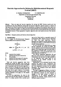
we consider a slightly different representation of these policies. In fact, unlike the classical representation (vector of policy-trees), we use a single decision tree for the entire group of agents, namely joint policy-tree and denoted δ. In the remainder of this paper, a joint policy-tree is a decision tree, where the root node α(δ) = (α(q1 ), · · · , α(qn )) is labeled by a joint action; arcs are tagged by joint observations; and subtrees are vectors of policy-trees η(δ, o) = (η(q1 , o1 ), · · · , η(qn , on )) from the last iteration. The right hand side of Figure 1 illustrates such a representation. The reader will note that this representation corresponds exactly to the policy-tree of the underlying MPOMDP.
3.2
Problem Reformulation
A desirable effect follows from the above observation: the problem of finding the optimal joint policy-tree δ t , for a given belief b and subtrees Qt−1 , is equivalent to the problem of determining joint action α(δ t ) and subtrees η(δ t , o) such that the resulting joint policy-tree δ t is both valid and optimal. A joint policy-tree is said to be valid if there exists a vector of policy-trees (q1 , · · · , qn ) which satisfies the following constraints (c1) and (c2): • (c1) α(δ) = (α(q1 ), · · · , α(qn )), • (c2) η(δ, o) = (η(q1 , o1 ), · · · , η(qn , on )). more precisely, δ t is a valid joint policy-tree if it corresponds to a unique vector of policy-trees. Otherwise, the joint policy-tree is said to be non-valid, when it is a policy-tree of the underlying MPOMDP that does not match to a vector of policy-trees.
3.3
The Heuristic Approach
At this point, we are left with two problems: first, how subtrees help us to compute the heuristic estimates of joint policies; moreover, how can these estimates be used to traverse our search space towards valid and useful joint policy-trees.
3.3.1
Computing the heuristic estimates
In order to compute the heuristic estimate of a joint policy-tree δ, for a given belief b and subtrees, we proceed as follows: select both joint action α(δ), and subtrees η(δ, o) that yield the highest contributions [9], where: • the contribution of subtree η(δ, o) is given by, P δ (3) gb,o = s0 P (s0 |b, δ, o)V (s0 , η(δ, o)) P 0 0 where P (s |b, δ, o) = s b(s)P (s |s, δ, o). The evaluation of all contributions requires a polynomial time. To better understand this complexity, let’s maxT rees be the maximum number of policy trees kept in memory for each agent at each horizon. We create |A||Ω|maxT rees|I| projections (in time O(|S|2 |A||Ω|maxT rees|I| )) that correspond to the number of allP possible contributions of subtree η(δ, o). Given the fact that i |Ωi | >> |I|, the complexity of this step is negligible in comparison to the complexity of the exhaustive backup. • finally, the exact value of joint policy-tree δ is, P P δ f (b, δ) = s∈S b(s)R(s, α(δ)) + o∈Ω gb,o
Figure 1:
MPOMDP
and DEC - POMDP joint policy-trees.
Since our goal is to determine a vector of policy-trees for a DEC it seems clear that the search space should be the space of vectors of policy-trees. However, for the sake of simplicity, POMDP ,
(4)
It is fairly easy, however, to demonstrate that the solution that consists in selecting, for each joint observation the subtree with the highest contribution, will lead in general to a non-valid joint policytree. Nevertheless, the good news is that the exact value of nonvalid joint policy-trees can be seen as a heuristic estimate of the exact value of valid joint policy-trees. More generally, joint policytrees of the underlying MPOMDP can be used to define an upperbound estimate of either partial or complete valid joint policy-trees.
Indeed, the heuristic estimate of a joint policy-tree is based on the decomposition of the evaluation function (Equation 1) into two estimates. The first estimate, g(b, δ), is the exact value coming from subtrees selected in accordance with (c2), i.e. valid subtrees. A non-valid subtree is therefore a subtree that does not satisfy (c2). The second estimate, h(b, δ), is the upper-bound value of the remaining subtrees selected in the order of their contribution, i.e. non-valid subtrees. We introduce Ω1 as the set of joint observations that leads to a valid subtree and Ω2 the remaining joint observations which means Ω = Ω1 ∪ Ω2 . This allows us to decompose the heuristic estimate of any joint policy-tree δ for a given belief b into the exact contribution coming from joint observations Ω1 , and the upper-bound of the completion Ω2 : X X b δ g¯α(δ),o g + f¯(b, δ) = b · rα(δ) + b,o o∈Ω2 o∈Ω1 (5) | {z } | {z } g(b,δ)
heuristic starts a new search tree with another joint action α(δ), until all joint actions have been selected. The resulting best joint policy-tree is then kept in memory. One can prioritize search trees in decreasing order of the heuristic estimate of their root nodes and prune all partially expanded joint policy-trees with heuristic estimates less or equal to the lower bound. The exact value of the joint policy-tree, that is both completely expanded (all subtrees are valid) and the current best joint policy-tree (that yields the highest exact value), can be set as the lower bound and denoted f (b).
h(b,δ)
b δ where g¯α(δ),o = maxδ gb,o and rα(δ) is a vector of R(s, α(δ)) for all s i.e., rα(δ) (s) = R(s, α(δ)). Of course, the heuristic estimate f¯ is an admissible heuristic function. Indeed, for any joint policy-tree δ and belief b the following holds by construction: f¯(b, δ) ≥ f (b, δ).
3.3.2
A Branch & Bound Method
In the following, we describe a straightforward heuristic solution to the problem of determining the best joint policy-tree given a belief state and subtrees. Our complete algorithm, that includes important enhancements to its straightforward counterpart, is discussed later. As suggested by [8], since A? can be viewed as a special case of Branch and Bound algorithm (B & B), one can resort our proposed approach to Branch and Bound instead. Similarly to POMDP incremental pruning techniques, the heuristic splits up the selection of the best joint policy-tree into the selection of several subtrees one for each joint observation o ∈ Ω. Unfortunately, as already mentioned a DEC - POMDP is a MPOMDP with additional constraints. Thus, in order to satisfy these constraint requirements, we combine the incremental pruning mechanisms to a heuristic search subroutine. The resulting heuristic method is able to efficiently walks through the search tree that represents the space of joint policy trees. As illustrated in the section of the search tree Figure 1, each node in the search tree is either a root node δ0 , an internal node δ1 , or a leaf node δ2 . A root node of a search tree is initialized with a joint policy-tree δ, where α(δ) can be any of the joint actions a ∈ A and η(o, δ) be the subtree with the highest contribution no matter if it is a valid subtree or not. Each internal node at depth h (h ≥ 1) of the search tree represents a joint policy-tree δ where only (h − 1) valid subtrees have been attached at δ’s leaf nodes (not to be confused with the leaf nodes of the search tree). Each joint policy-tree at leaf node of the search tree, where valid subtrees have been attached, is a valid joint policy-tree. Notice that during the course of the search, leaf nodes of the the search tree that do not represent a valid joint policy-tree turn out to be either the root node or future internal nodes of the search tree. What PBIP does, is evaluate leaf nodes of the search tree, select the node with the highest heuristic estimate, and expand this node, thus descending one step further in the search tree. The search then proceeds by expanding joint policy-trees δ at leaf nodes of the search tree in descending order of f¯-values, until the best solution is identified. Expanding a leaf node consists in expanding the attached joint policy-tree δ, which means: building all possible joint policy-trees that extend δ by replacing one non-valid subtree by one valid subtree; then making the resulting joint policy-trees as child nodes of δ. When a search tree has been completely explored, the
Figure 2: A section of PBIP search tree.
4.
PBIP ALGORITHM
The heuristic method discussed above suffers from three major drawbacks: computation overhead, memory overhead, and inefficiency of the pruning strategy. To overcome these drawbacks, we suggest additional optimizations.
4.1
Reducing computation overhead
First of all, the above heuristic requires checking whether or not (c2) and (c1) are satisfied for each joint policy-tree δ. However, checking (c2) incurs significant computation overhead since it re-
quires in the worst case a time complexity O(n · |Ω1 | · |Qt−1 |), where a single subtree requires O(n · |Ω1 |) operations. To handle this issue we rely on the fact that only a few non-valid subtrees of a joint policy-tree δ have to be replaced by valid subtrees to build a valid joint policy-tree as illustrated in the example below. E XAMPLE 1. Back to the example of Figure 1, given two valid subtrees of δ, η(δ, (o0 , o0 )) = (qi2 , qj2 ) and η(δ, (o1 , o1 )) = (qi1 , qj1 ). Then, using (c2) it turns out that η(qi , o0 ) = qi2 and η(qi , o1 ) = qi1 for agent i; η(qj , o0 ) = qj2 and η(qj , o1 ) = qj1 for agent j . Therefore, the complete joint policy-tree δ is built as follows: η(δ, (o0 , o1 )) = (η(qi , o0 ), η(qj , o1 )) = (qi2 , qj1 ). Doing so permits us to reduce the computation overhead since (c2) is checked only for a small number of subtrees. As discussed
in the following, even for those subtrees it is not always required to check (c2). More formally, we introduce the basis joint policy-tree as the smallest partial joint policy-tree, where some arcs have been removed, that is sufficient to recover the complete joint policy-tree. The set of joint observations, which tag the arcs of a basis joint policy-tree is referred to as the set of basis joint observations and denoted ΩB . The nodes labeled with subtrees executed after receiving basis joint observations are called basis nodes. In Figure 1, the
joint policy-tree, where arcs {(o0 , o1 ), (o1 , o0 )} are removed from δ, is a basis joint policy-tree, its basis joint observations and basis nodes are sets {(o0 , o0 ), (o1 , o1 )} and {(qi2 , qj2 ), (qi1 , qj1 )}, respectively. While it is fairly easy to find a joint policy-tree using a basis joint policy-tree, one may ask how to determine a basis joint policytree. One simple way to determine a basis joint policy-tree is first to build the set of basis joint observations ΩB then select a subtree for each basis leaf nodes. We build ΩB by progressively adding a new joint observation o ∈ Ω, which is component-wise different or simply different from joint observations already added into ΩB , e.g. joint observations (o0 , o0 ) and (o1 , o1 ) are componentwise different while (o1 , o0 ) and (o1 , o1 ) are simply different since their first components are equal. We add joint observations that are component-wise different first then complete with simply different joint observations until ΩB is a basis. The nice property of the idea of ‘working with basis joint policy-trees’ lies in the fact that it reduces the number of times (c2) has to be checked. Indeed, (c2) is satisfied for joint observations that are component-wise different. In addition, we can prove that the number of basis nodes κ is quite small, κ := maxi∈I |Ωi | (by construction of ΩB ). To get a better insight of the basis set, one can look at ΩB as the smallest set of joint observations where each individual observation is included in at least one joint observation of that set. In particular, if all agents have the same number of individual observations, we can forget about (c2), i.e. joint observations that are component-wise different define the basis set ΩB .
4.2
Reducing space complexity.
One major drawback with either A? -style heuristics or B & B-like techniques is that in the worst case they remember an exponential number of nodes. Indeed, in both, branching rules to be applied can be seen as subdivision of a part of the search space. Generating subspaces are then kept in memory. Unfortunately, this incurs considerable memory requirement. To cope with this, we restrict the set of possible nodes at a given depth of the search tree, as illustrated in Figure 2. To do so, our search tree is built such that joint policy-trees that can be attached at leaf nodes are all possible assignments of subtrees to the same basis node. This idea is motivated by the observation that such joint policy-trees differ only from the last subtree assigned to them, see for example δ1 and δ4 . As a result, they are processed in decreasing order of the contribution of the last subtree assigned to them, e.g., (qi2 , qj2 ) and (qi1 , qj2 ) respectively. Moreover, contributions of subtrees are stored in a priority stack that will maintain subtrees in descending order. Then, to expand leaf node δ1 , we only need to build the best child node δ2 , i.e. basis joint policy-tree where the last assigned subtree (qi2 , qj2 ) yields the highest contribution. Indeed, the remaining child nodes will be progressively built in decreasing order of the contribution of the subtree assigned to them if necessary. A straightforward implementation of PBIP’s search tree will results in a linear memory space O(κ). In particular, our PBIP implementation (see subsection 4.4) only needs to keep one node that is progressively updated. Since the space complexity plays a major role in B & B performances, we compare PBIP to B & B techniques with different search strategies of selecting the next node: Best First (BeFS); Breadth First (BFS) and Depth First (DFS). Indeed, the strategy for selecting the next node to process usually reflects a trade-off between keeping the number of processed nodes in the search tree low, and staying within the memory capacity of the computer used. Although the DFS strategy is slightly better than BeFS and clearly better than BFS , not surprisingly PBIP is superior to all of them in all tested benchmarks. The reason turns out to be that, PBIP shares common
skills with BeFS and DFS.
4.3
Improving the pruning strategy
Using basis joint policy-trees, we are able to improve significantly the pruning strategy by means of exploiting f¯’s properties. Let us denote S UCC(δ) the set of successor joint policy-trees of a joint policy-tree δ, i.e. child and brother nodes of δ built after δ. For example in Figure 2, the successor joint policy-trees of δ1 are {δ2 , δ3 , δ4 }. The admissibility of the heuristic function f¯ and the order in which PBIP processes joint policy-trees allow us to state the following results. L EMMA 1. Let δ be a joint policy-tree. Then, the following holds: ∀δ 0 ∈ S UCC(δ) : f¯(b, δ) ≥ f¯(b, δ 0 ). P ROOF. We only need to prove this claim for child nodes, since by hypothesis δ yields a better heuristic estimate than its brother nodes include into S UCC(δ). We proceed by induction. First, the basis case consists in proving that the next partial or complete joint policy-tree δ1 that extends δ is such that: f¯(b, δ) ≥ f¯(b, δ1 ). To do so, we need to look at what is new in δ1 according to δ. The main difference lies in the fact that δ1 has one more subtree assigned to a basis node leading from basis joint observation, e.g. o1 : f¯(b, δ1 )
δ1 b = f¯(b, δ) − g¯α(δ),o 1 + gb,o1 δ1 b = f¯(b, δ) − g¯α(δ1 ),o1 + gb,o 1 ≤ f¯(b, δ)
(α(δ) = α(δ1 ))
δ1 b The last inequality holds since g¯α(δ 1 ≥ gb,o1 by definition 1 ),o of the upper-bound. By repeating this argument for any consecutive pair (δk , δk+1 ) ∈ S UCC(δ) × S UCC(δ), the following holds: f¯(b, δk ) ≥ f¯(b, δk+1 ), ∀k = 1, · · · , |S UCC(δ)| . This proves the above Lemma.
Intuitively, it is obvious that this property is a more strict requirement than monotonicity since S UCC(δ) also includes δ’s brother nodes. Using this property and the order PBIP processes joint policytrees, we establish the following theorem. This theorem describes an efficient property used to avoid joint policy-trees with low heuristic estimate. T HEOREM 1. Let δ be a joint policy-tree with heuristic estimate f¯(b, δ), and δ 0 the current best joint policy-tree. If f¯(b, δ) ≤ f (b, δ 0 ), then the following holds: f (b, δ 0 ) ≥ f (b, δk ), ∀δk ∈ S UCC(δ). P ROOF. In accordance with Lemma 1 we have, f¯(b, δ) ≥ f¯(b, δk ), ∀δk ∈ S UCC(δ) Then, the following holds: f (b, δ 0 ) ≥ f¯(b, δ) (by hypothesis) ≥ f¯(b, δk ), ∀δk ∈ S UCC(δ) (Lemma 1) ≥ f (b, δk ), ∀δk ∈ S UCC(δ) (upper-bound def.) This theorem states only that if a joint policy-tree δ has a heuristic estimate less or equal to the current lower-bound, PBIP does not build subspace S UCC(δ). This strategy improves the pruning strategy used in A? -style algorithms since it does not require all successor nodes S UCC(δ) to be generated and evaluated. From a practical point of view, if δ’s heuristic estimate is less or equal to the current lower bound (backtracking condition), then there are two possibilities: (a) if δ’s parent node is the root node, then the search terminates; (b) otherwise, the search backtracks to δ’s parent node and tests the backtracking condition.
Algorithm 1 PBIP subroutines. 1: procedure S EARCH((b, a, δ t , ΩB , Qt−1 , Selectt )) 2: open ← EmptyStack, k ← 0 3: α(δ) ← a δ , g b 4: ∀(o, η(δ, o)) ∈ Ω × Qt−1 : compute gb,o ¯a,o 5: 6: 7: 8: 9: 10: 11: 12: 13: 14: 15:
EXPAND . initialize the search tree while open 6= EmptyStack do k k (o , η(δ, o )) ← open.PEEK if f (b) < f¯(b, δ) then if ok = oκ then if f (b, δ) > f (b) and δ 6∈ Selectt then δt ← δ f (b) ← f (b, δ t ) EXPLORE
else EXPAND else BACKTRACK
. select a new subtree η(δ, ok ) . assign a subtree η(δ, ok+1 ) . backtrack if pos. to η(δ, ok−1 )
E XAMPLE 2. Figure 2 shows the progress of PBIP to find the best joint policy-tree for the search tree associated with joint action (a2 , a2 ). The first node to be built starting from root node (δ0 ) is δ1 , because it yields the highest heuristic estimate −4. This node in turn generates only one child node, i.e. δ2 . Since the resulting joint policy-tree has non-empty basis nodes, PBIP computes its exact value −4, and uses it as a lower bound. Then, PBIP backtracks to node δ1 . Because δ1 ’s heuristic estimate −4 is equal to the current lower bound, PBIP does not build its successor nodes δ3 and δ4 . Then, the search terminates since δ1 ’s parent node (δ0 ) is the root node of the search tree. Finally, joint policy-tree δ2 is the best one for this search tree.
4.4
1: procedure EXPAND 2: k ←k+1 . go forward to η(δ, ok+1 ) 3: η(δ, ok ) ← EXPLORE 4: open.PUSH(ok , η(δ, ok )) 5: procedure BACKTRACK 6: if open.IS N OT E MPTY then 7: (ok , −) ← open.POP 8: η(δ, ok ) ← −1 . reinitialize the pointer position 9: if ok 6= o1 then 10: k ←k−1 . go backward to η(δ, ok−1 ) 11: EXPLORE 12: procedure EXPLORE 13: INCREMENT (η(δ, ok )) 14: if η(δ, ok ) > |Qt−1 | then 15: BACKTRACK . backtrack if pos. to η(δ, ok−1 ) k 16: return η(δ, o )
Specific implementation
In the same vein as MBDP, PBIP combines the bottom-up and top-down heuristic methods as described in Algorithm 2. However, what sets PBIP apart from MBDP is its ability to avoid the exhaustive generation of all possible joint policy-trees at each iteration. Indeed, a single iteration of PBIP can be summarized in the following steps: first, the algorithm sets the joint policy-tree from the last iteration Qt−1 . Next, it chooses top-down heuristics from the portfolio H in order to generate maxT rees number of belief states. Then, it uses subroutine S EARCH to determine the set of best joint policy-trees Selectt for the set of generated belief states. Finally, at iteration T , the best joint policy-tree with respect to the initial belief state b0 is returned. Algorithm 2 Point based incremental pruning 1: procedure PBIP((maxT rees, T , H)) 2: Select1 ← initialize all depth-1 joint policy-trees 3: for all t = 2, · · · , T do 4: Qt−1 ← Selectt and Selectt ← ∅ 5: for all k = 1, · · · , maxT rees do 6: chooses h ∈ H and generate belief b 7: δ t ← null and f (b) ← −∞ 8: for all a ∈ A do 9: S EARCH(b, a, δ t , ΩB , Qt−1 , Selectt ) 10: add best joint policy-tree δ t to Selectt 11: select the optimal joint policy-tree δ ?T from SelectT 12: return δ ?T In the following, we draw attention to a single search tree of PBIP with the following entries: a belief state b; a joint action a, the current best joint policy-tree δ t , the set of basis joint observations ΩB , subtrees from the last iteration Qt−1 , and finally current best joint policy-trees Selectt (Algorithm 1). Exact and upper bound
contributions of subtrees in Qt−1 are computed and stored in a priority queue. We use η(δ, o) as either a subtree or its index position in the priority queue interchangeably. Therefore, PBIP’s S EARCH subroutine can be summarized in the following steps: First of all, S EARCH initializes an open list ‘open’ that will contain the expanded nodes. Second, it expands the current leaf node of the search tree that yields the highest heuristic estimate (see procedure EXPAND, lines 1-5). Then, S EARCH goes through the main loop. Each loop consists in evaluating the heuristic estimate of the current either partially or completely expanded joint policytree (lines 6-19). If the heuristic estimate is less or equal to the lower bound (line 8), then S EARCH backtracks (if possible) to the last expanded joint policy-tree (see procedure BACKTRACK, lines 6-15). Otherwise, it updates the best joint policy-tree if it is complete and its exact value is greater than the lower bound (lines 9-13) and explores any remaining alternatives (see procedure EXPLORE, lines 16-22). If not, S EARCH backtracks and expands the current joint policy-tree δ (see procedure EXPAND, lines 1-5) by assigning a subtree η(δ, ok+1 ). Note that, the new best joint policy-tree has to be component-wise different from those already selected (line 10). This enables us to avoid the problem of selecting identical policytrees for each agent. Finally, the search ends when the root node of the search tree has been completely explored.
5.
THEORETICAL PROPERTIES
In this section, we introduce some additional theoretical properties that guarantee PBIP performances, including completeness, optimality, and complexity. T HEOREM 2.
PBIP
heuristic method is complete.
P ROOF. PBIP will eventually terminate in the worst case after enumerating all possible joint policy-trees from the current iteration given the set of subtrees, which means after visiting the entire exponential space of joint policy-trees at each iteration. The best solution δ for a given belief b will be the one that yields the highest exact value f (b, δ). T HEOREM 3. PBIP heuristic method is optimal with respect to a given belief and the set of subtrees. One can look at PBIP as an A? -style algorithm. Indeed, complete joint policies in best-first fashion following an admissible heuristic function f¯. Then, if PBIP terminates and returns a joint policy-tree δ, the convergence property of A? and the admissibility of the heuristic f¯ guarantee the optimality of the solution with respect to a given belief b and subtrees. P ROOF. PBIP visits
Algorithm (T )
HORIZON
MBDP - OC PBIP (sec.) AEV CPU (sec.) AEV CPU (sec.) problem maxT rees = 3 90.29 0.190 N.A. N.A. 90.29 0.060 900.29 2.270 N.A. N.A. 900.29 0.940 9000.29 51.93 N.A. N.A. 9000.29 38.48 MA - TIGER problem maxT rees = 20 12.5±2.9 67.1±0.13 N.A. N.A. 13.6±1.11 5.55±0.88 25.8±2.1 159±0.16 N.A. N.A. 26.8±1.50 15.1±2.68 73.9±0.7 438±0.86 N.A. N.A. 74.2±2.76 45.3±6.49 149 901 N.A. N.A. 147±5.84 94.2±9.53 COOPERATIVE BOX - PUSHING problem maxT rees = 3 maxObs = 3 N.A. 99.59 7994.6 89.94 7994.4 102.5±6.46 11.8±3.61 N.A. 102.6 17031 135.0 17194 198.0±10.8 25.0±4.21 N.A. 82.99 44708 272.70 44210 422.2±20.8 61.6±10.6 N.A. 73.88 89471 440.08 90914 786.4±31.9 113±20.8 AEV = average expected value N . A . = not applicable % = pourcentage of expanded nodes MBDP
AEV
IMBDP
CPU
(sec.)
AEV
CPU
%
MABC
100 1000 10000 10 20 50 100 10 20 50 100
39 38 38 7.83 12.4 15.3 12.9 10.9 10.3 9.07 9.62
Table 1: Performances of all PBIP, MBDP, IMBDP and MBDP - OC. Notice that in the worst case PBIP still has an exponential time complexity with respect to the number of agents and κ: in the best case, however, its time complexity is O(κ). The proof of these results relies on the following observations: first, since PBIP eventually enumerates all possible joint policies at a given iteration, in the worst case its time complexity is also exponential; but in the best case, PBIP requires only κ steps to build the first complete joint policy-tree. Nevertheless, its overall time complexity can be influenced by the pre-computing step that requires roughly O(|S 2 ||A||Ω|maxT rees|I| ) operations. Although PBIP is based on A? algorithm, it incurs negligible memory overhead. Indeed, the subroutine S EARCH has a linear space complexity O(κ), i.e. the length of the longest path from the root node to the best joint policy-tree. This is possible since we compute all contributions of subtrees for all joint action and joint observation pairs before the search starts. As a result, the overall space complexity of PBIP is O(|A||Ω|maxT rees).
6.
EXPERIMENTS
As MBDP and its extensions are known to perform better than other approximate algorithms such as point based dynamic programming (PBDP), we compare PBIP only to MBDP, IMBDP and MBDP - OC . Comparison is made according to DEC - POMDP benchmarks from the literature: the multi-access broadcast channel (MABC) problem [6], the multi-agent tiger problem [7] and the COOPERA TIVE BOX - PUSHING problem [11]. The COOPERATIVE BOX - PUSHING problem provides an opportunity for testing the scalability of different algorithms. We executed the algorithms using the same parameter controls of the selection of heuristics from the portfolio, maxT rees, recursion depth (set at 1) and maxObs. Except that parameter maxObs is only used for IMBDP and MBDP - OC solvers. Table 1, Figure 3 and Figure 4 present our experimental results. For each problem and method we report: The average expected value (AEV.) – this is because both MBDP and PBIP are partly randomized then selected belief states and thus the quality of the resulting solution may differ from one trial to another. Execution time – we report only the CPU time (in seconds) since all algorithms are coded in JAVA, properly optimized and run on the same machine. PBIP , where Ni denotes Expanded nodes (%) – where % = 100 × NNMBDP the number of expanded joint trees by algorithm i. This value helps to estimate the benefits of our pruning heuristic.
6.1
Discussion
Table 1 presents performance results of all the algorithms on the three benchmarks. As we already notice, both PBIP and MBDP algorithms are likely to find the same solution, since they differ only in the way they select the best joint policy-trees. Our results clearly indicate that PBIP is faster than MBDP, IMBDP or MBDP - OC and scales up better. For problem with small number of observation both PBIP and MBDP provide approximately the same solution
quality, but the time required by PBIP to reach the desired solution is always faster. For example, the MABC problem for horizon 1000 is solved (approximately) in 560 seconds with PBIP whereas MBDP requires 1094 seconds to solve it. The most impressive results rely on the percentage of expanded joint policy-trees. For instance, in the MA - TIGER problem at horizon 10, PBIP expands only 7.83% of what would be expanded by a brute force approach. However, when the horizon increases in general this percentage also increases and then stabilizes depending on the problem and parameter maxT rees. Table 1 via the COOPERATIVE BOX - PUSHING problem also presents a more focused comparison of the relative ability of the PBIP and MBDP extensions to scale up. Overall, it appears that IMBDP and MBDP - OC are slowed down considerably by the exhaustive backup computation and the management of the resulting joint policy-trees. PBIP, however, benefits from its ability to identify subspaces of joint policy-trees with low heuristic estimate, this enables it to focus only on a small space of relevant joint policytrees. Even though PBIP does not include an observation compression subroutine, it solves the COOPERATIVE BOX - PUSHING up to 800 times faster than IMBDP and MBDP - OC, while providing a better solution quality, that is up to 1.78 times higher than the MBDP OC ’s and up to 10 times higher than the IMBDP’s. Notice that given the time requires to build policies using either IMBDP or MBDP OC their results are not averaged, so the solution quality may be slightly different from one trial to another. These differences become more pronounced as the parameter maxT rees increases. As pointed out by [12], by increasing parameter maxT rees one generally increases both solution quality and runtime. We illustrate the performance of MBDP and PBIP when one increases parameter maxT rees for the MA - TIGER problem. On the right hand side, Figure 3 shows the runtimes of both MBDP and PBIP when parameter maxT rees is increased. On the left hand side, it shows the solution value for different values of parameter maxT rees. The purpose of Figure 3 is therefore to show how both PBIP and MBDP perform for different values of parameter maxT rees. As illustrated, MBDP exceeds the time limit (1 hour) for maxT rees = 35 while PBIP is able to solve the MA TIGER problem using maxT rees = 100 and more. Doing so enables PBIP to improve the solution quality of MA - TIGER problem. Nevertheless, even though PBIP avoids a large number of joint policy-trees, the benefits do not fully manifest in total execution time. For instance in Table 1, for MABC problem at horizon 10000, PBIP explores only 38% of the joint policy-trees, however, it took 38.48 seconds to find the best solution, while MBDP required 51.93 seconds. This is mainly because computing exact and upperbound estimates of each subtree incurs considerable computation overhead. Of course, managing those estimates requires a number of costly operations including: subtrees re-ordering, checking the validity of a given joint policy-tree. We believe that those issues would be overcome by an appropriate data structure and/or imple-
MBDP PBIP
3000
14 Solution Quality
Execution Time (seconds)
16 3500
2500 2000 1500 1000 500
12 10 8 6 4 2
0
PBIP
0 10
20
30 40 50 60 70 Maximum Number of Trees
80
90
100
10
20
30 40 50 60 70 Maximum Number of Trees
80
90
100
Figure 3: Performances for MA - TIGER problem with T = 10. 130 125 4
PBIP
Solution Quality
Execution Time (log10 sec.)
5
3 2 1
120
PBIP
115 110 105 100 95
0
90 2
3
4
5 6 7 8 Maximum Number of Trees
9
10
2
3
4
5 6 7 8 Maximum Number of Trees
9
10
Figure 4: PBIP’s performances for COOPERATIVE BOX - PUSHING problem with T = 10. mentation. To confirm the scalability of PBIP, we increase parameter maxT rees up to 7, in the COOPERATIVE BOX - PUSHING problem (see Figure 4). We only report the PBIP’s performances since IMBDP and MBDP - OC quickly run out of time (10 hours). Overall, it appears that although PBIP scales up better than other approximate DEC-POMDP solvers, the impact of increasing maxT rees parameter is not negligible. For example, if maxT rees = 7 PBIP requires approximately 8 hours while requiring only one hour and half when using maxT rees = 6. Roughly, the running time grows exponentially with parameter maxT rees while the average solution quality grows only about 5% for each additional trees.
7.
CONCLUSION AND FUTURE WORK
We have presented PBIP, the first heuristic method that circumvents the problem of generating and evaluating all possible joint policy-trees at each iteration of DEC - POMDP solvers. This algorithm is based on two observations: (1) most joint policy-trees resulting from the exhaustive backup yield low heuristic estimate; (2) the DEC - POMDP policy space is a subspace of the MPOMDP policy space. This insight, allows PBIP to conduct a search towards the most promising joint policies, and avoids the irrelevant ones. Experiment results show orders of magnitude improvement in the performance of all leading algorithms including MBDP and its extensions. Although the proposed approach has been illustrated within the MBDP framework, PBIP can easily be used to scale up others DEC - POMDP solvers for either finite or infinite cases. Currently, we are tracking others similarities between DEC - POMDP and POMDP models so as to reduce the algorithmic gap that separates these two closely related problems and hopefully to enable us to scale up to real-life applications.
Acknowledgments We would like to thank Sven Seuken and Alan Carlin for making available their MBDP, IMBDP and MBDP - OC codes for solving finite horizon DEC - POMDPs. We also thank Hamid R. Chinaei and Camille Besse for the helful comments on this work.
8.[1] R.REFERENCES E. Bellman. Dynamic Programming. Dover Publications, Incorporated, 1957.
[2] D. S. Bernstein, R. Givan, N. Immerman, and S. Zilberstein. The complexity of decentralized control of markov decision processes. Math. Oper. Res., 27(4), 2002. [3] C. Besse and B. Chaib-draa. Parallel rollout for online solution of dec-pomdps. In FLAIRS Conference, pages 619–624, 2008. [4] A. Boularias and B. Chaib-draa. Exact dynamic programming for decentralized pomdps with lossless policy compression. In ICAPS, pages 20–27, 2008. [5] A. Carlin and S. Zilberstein. Value-based observation compression for DEC-POMDPs. In AAMAS, 2008. [6] E. A. Hansen, D. S. Bernstein, and S. Zilberstein. Dynamic programming for partially observable stochastic games. In AAAI, pages 709–715, 2004. [7] R. Nair, P. Varakantham, M. Tambe, and M. Yokoo. Networked distributed POMDPs: A synthesis of distributed constraint optimization and POMDPs. In AAAI, pages 133–139, 2005. [8] D. S. Nau, V. Kumar, and L. Kanal. General branch and bound, and its relation to a* and ao*. Artif. Intell., 23(1):29–58, 1984. [9] J. Pineau, G. Gordon, and S. Thrun. Point-based value iteration: An anytime algorithm for POMDPs. In IJCAI, 2003. [10] Z. Rabinovich, C. V. Goldman, and J. S. Rosenschein. The complexity of multiagent systems: the price of silence. In AAMAS, pages 1102–1103, 2003. [11] S. Seuken and S. Zilberstein. Improved Memory-Bounded Dynamic Programming for DEC-POMDPs. In UAI, 2007. [12] S. Seuken and S. Zilberstein. Memory-bounded dynamic programming for DEC-POMDPs. In IJCAI, pages 2009–2015, 2007. [13] D. Szer and F. Charpillet. Point-based dynamic programming for DEC-POMDPs. In AAAI, pages 16–20, July 2006. [14] D. Szer, F. Charpillet, and S. Zilberstein. Maa*: A heuristic search algorithm for solving decentralized POMDPs. In UAI, pages 568–576, 2005. [15] P. Varakantham, J. Marecki, M. Tambe, and M. Yokoo. Letting loose a spider on a network of POMDPs: Generating quality guaranteed policies. In AAMAS, May 2007.