applied sciences Article
Pollutant Recognition Based on Supervised Machine Learning for Indoor Air Quality Monitoring Systems Shaharil Mad Saad 1, * ID , Allan Melvin Andrew 2 , Ali Yeon Md Shakaff 3 , Mohd Azuwan Mat Dzahir 1 , Mohamed Hussein 1 , Maziah Mohamad 1 and Zair Asrar Ahmad 1 1 2 3
*
Faculty of Mechanical Engineering, Universiti Teknologi Malaysia (UTM), Johor Bahru 81310, Malaysia;
[email protected] (M.A.M.D.);
[email protected] (M.H.);
[email protected] (M.M.);
[email protected] (Z.A.A.) Center for Diploma Studies (CDS), Universiti Malaysia Perlis (UniMAP), Kampus UniCITI Alam, Chuchuh, Padang Besar 02100, Malaysia;
[email protected] Center of Excellence for Advanced Sensor Technology (CEASTech), Universiti Malaysia Perlis (UniMAP), Taman Muhibbah, Jejawi, Arau 02600, Malaysia;
[email protected] Correspondence:
[email protected]; Tel.: +60-7-553-4673
Received: 3 July 2017; Accepted: 8 August 2017; Published: 11 August 2017
Abstract: Indoor air may be polluted by various types of pollutants which may come from cleaning products, construction activities, perfumes, cigarette smoke, water-damaged building materials and outdoor pollutants. Although these gases are usually safe for humans, they could be hazardous if their amount exceeded certain limits of exposure for human health. A sophisticated indoor air quality (IAQ) monitoring system which could classify the specific type of pollutants is very helpful. This study proposes an enhanced indoor air quality monitoring system (IAQMS) which could recognize the pollutants by utilizing supervised machine learning algorithms: multilayer perceptron (MLP), K-nearest neighbour (KNN) and linear discrimination analysis (LDA). Five sources of indoor air pollutants have been tested: ambient air, combustion activity, presence of chemicals, presence of fragrances and presence of food and beverages. The results showed that the three algorithms successfully classify the five sources of indoor air pollution (IAP) with a classification rate of up to 100 percent. An MLP classifier with a model structure of 9-3-5 has been chosen to be embedded into the IAQMS. The system has also been tested with all sources of IAP presented together. The result shows that the system is able to classify when single and two mixed sources are presented together. However, when more than two sources of IAP are presented at the same period, the system will classify the sources as ‘unknown’, because the system cannot recognize the input of the new pattern. Keywords: indoor air quality; supervised machine learning; pollutants recognition
1. Introduction The issue of outdoor air pollution (OAP), such as haze, is well known to the public due to the attention given to it by the media. In contrast, the issue of indoor air pollution (IAP) is less known to the public, although IAP poses similar threats towards human health. In fact, more attention should be given to the issue of IAP, because people normally spend 90% of their time in indoor environments [1]. IAP, which undermines indoor air quality (IAQ), is found to contain indoor air pollutants such as harmful gases and contaminants at a concentration level up to five times higher than the concentration of these pollutants in normal air. In severe cases, the concentration level of the pollutants could rise up to 100 times more than a normal concentration level, which is hazardous for human health [1]. IAP can be defined as the disturbance of any gases, materials or human activities on the state of ambient air in indoor environment [2]. In other words, IAP does not need the presence of disease or infirmity. As long as the concentration in the normal ambient air is disturbed either by gases, other materials or combustion activity, it is already considered as pollution. The most common sources Appl. Sci. 2017, 7, 823; doi:10.3390/app7080823
www.mdpi.com/journal/applsci
Appl. Sci. 2017, 7, 823
2 of 21
of IAP are contributed by combustion activities such as cigarette smoking, wood or paper burning, gas stoves, gas-fired dryers and engines emission [3,4]. Other materials, such as chemical products, building materials and office materials, are also major sources of IAP. Chemical products such as air fresheners and cleaning products contribute to IAP by emitting volatile organic compounds (VOCs), while building and office materials such as printers and carpets also release air contaminants such as dust into the indoor air atmosphere [5–9]. IAP may also emerge as a result of variations of gas concentration in the indoor air, as well as from variations in thermal conditions such as temperature and humidity [10,11]. Thermal or physical conditions such as temperature, relative humidity (RH) and air movement are important IAP parameters as they could affect people’s perception towards IAP. These physical parameters can act directly on building occupants, interact with indoor air pollution factors or affect human responses to the indoor environment [12–16]. These sources of IAP might not look harmful, but to a certain extent (based on the concentration level) they may be hazardous to human health. The health effects from IAP may be experienced soon after exposure, or possibly, years later, depending on the individuals and type of pollutants they have been exposed to [17]. The common health conditions that may show up immediately include irritation of the eyes, nose, and throat, headaches, dizziness, fatigue, asthma and humidifier fever. The health effects of years of exposure to IAP are more dangerous and can be fatal; these include some respiratory-related diseases, heart disease, and cancer [18,19]. The health effects relating to poor indoor air quality have been divided into four categories: environmental tobacco smoke (ETS), sick building syndrome (SBS), building related illness (BRI), and thermal comfort problems (TCP) [10,13,20]. Hence, meticulous attention should be given to make sure the indoor air is safe and comfortable. Indoor air may be polluted by various types of pollutants which may come from cleaning products, construction activities, perfumes, cigarette smoke, water-damaged building materials and outdoor pollutants [21]. Although these gases are usually safe for humans, they could be hazardous to human beings, especially people with respiratory-related problem and children, if their amount exceeded certain limits of exposure for human health. In terms of the current technology, certain sensing devices have allowed researchers to get continuous, quick and reliable information about ambient air [21] which enable advanced data processing to be applied to the data of ambient air. Forecasting techniques allow the system to predict level of IAQ while pattern recognition techniques allow the system to recognize certain types of smell. However, these advanced data processing techniques were mainly used to investigate the odour in outdoor environments [22–25]. In indoor environments, odour recognition was usually used to detect odour from a single category; for example, the use of odour recognition to recognize types of mushrooms [26], types of oil flowers (lavender, hyssop, geranium and rosemary) [27] or types of pure chemical only (ethanol, hexanal, linalool, and ammonia) [28]. On the other hand, some other techniques, such as computational fluid dynamics (CFD), are used to predict IAP in indoor environments [29,30]. CFD is used to evaluate the IAQ for buildings near to the road traffic environment. This study proposed an enhancement of the IAQMS, where the system is integrated with sources of pollution recognition. The proposed IAQMS has been developed and designed using an array of sensors which can also effectively function as an electronic nose, meaning that it could measure multiple pollutants that influenced indoor air levels. The pattern recognition algorithm allows the system to recognize the sources of IAP from five conditions: ambient air, combustion activity, presence of fragrance, presence of chemical and presence of food and beverages. As for the sources influencing IAP recognition ability, this study utilized a machine learning algorithm that is widely used in data mining. In order to find the best classifier among the family of machine learning algorithms, three algorithms which have been used in many applications—especially involving odour or smell classification—have been chosen. The three algorithms chosen are multilayer perceptron (MLP), K-nearest neighbour (KNN) and linear discrimination analysis (LDA). Then, the classifier that provided the best classification results is chosen to be embedded into the system.
Appl. Sci. 2017, 7, 823
3 of 21
Appl. Sci. 2017, 7, 823
3 of 21
2. Overview of Developed IAQMS System 2. Overview of Developed IAQMS System
Basically, the developed system consists of the sensor module cloud (SMC), base station and Basically,client, the developed system consists of the sensormodule module cloud cloud (SMC), station and service-oriented as shown in Figure 1. The sensor (SMC) base contains collections service-oriented client, as shown in Figure 1. The sensor module cloud (SMC) contains collections of base of sensor modules that measure the air quality data and transmit the captured data to the sensor modules that measure the air quality data and transmit the captured data to the base station station through a wireless network. Each sensor module includes an integrated sensor array that through a wireless network. Each sensor module includes an integrated sensor array that can can measure IAQ parameters. There are various IAQ parameters involved in measuring the IAQ measure IAQ parameters. There are various IAQ parameters involved in measuring the IAQ level. level.These Theseparameters parameters are divided into four categories: physical condition, chemical contaminants, are divided into four categories: physical condition, chemical contaminants, biological contaminants, andand other common IAQIAQ parameters. However, forfor thethe purpose of of thisthis project, biological contaminants, other common parameters. However, purpose only nine parameters have been chosen, which are nitrogen dioxide (NO ), carbon dioxide (CO ), project, only nine parameters have been chosen, which are nitrogen dioxide (NO2), carbon dioxide 2 2 ozone (O3 ), (CO carbon monoxide (CO), oxygen (O2(CO), ), VOCs and (O particulate matter (PM10 ) matter along with 2), ozone (O3), carbon monoxide oxygen 2), VOCs and particulate (PM10temperature ) along with temperature and chooses humidity.the This study chooses theIAQMS parameters foron itsthe IAQMS based on the and humidity. This study parameters for its based indoor air parameters indoor air parameters highlighted by the Occupational Safety and Health Administration (OSHA), highlighted by the Occupational Safety and Health Administration (OSHA), the American Society of the American Society Heating, Refrigerating and Air-Conditioning (ASHRAE), the Heating, Refrigerating andofAir-Conditioning Engineers (ASHRAE), the Engineers United States Environmental United States Environmental Protection Agency (US EPA) and Malaysian regulations on indoor air Protection Agency (US EPA) and Malaysian regulations on indoor air as stipulated by Department of as stipulated by Department of Occupational Safety and Health (DOSH) [12,17,31,32]. Occupational Safety and Health (DOSH) [12,17,31,32].
Figure 1. System architecture indoorair airquality quality (IAQ) monitoring. Figure 1. System architecturefor forreal-time real-time indoor (IAQ) monitoring.
sensor divided intothree threetypes types of sensor: particle sensor and and thermal The The sensor cancan be be divided into sensor:gas gassensor, sensor, particle sensor thermal sensor. Lists of sensors used in the proposed system along with their operational range are presented sensor. Lists of sensors used in the proposed system along with their operational range are presented in Table 1 below. in Table 1 below. Table Listof ofsensors sensors used Table 1.1.List usedininthe thesystem. system. No
Sensor Model
No 1 Sensor Model CDM 4161
Electrochemical MOX MOX Electrochemical MOX MOX MOX MOX Electrochemical MOX Thermal Electrochemical 7 Thermal Thermal HSM20G 7 8 GP2Y1010AU0F Optical Thermal 8 GP2Y1010AU0F Optical
1 2 3 4 5 6
2 3 4 5 6
TGS4161 5342 CDM TGS 2602 TGS 5342 MiCS-2610 TGS 2602 MiCS-2710 MiCS-2610 KE-25 MiCS-2710 KE-25 HSM20G
Sensor Type
Sensor Type MOX
Target Parameter CO CO 2 VOCs CO O3 VOCs NO O3 2 O22 NO Humidity O2 Temperature Humidity PM10 Temperature
Typical Detection Range Typical Detection 400–2000 ppm Range 0–100 ppm 400–2000 ppm 0–30 0–100ppm ppm 0–1 0–30ppm ppm 0.05–5 ppm 0–1 ppm 0–100% 0.05–5 ppm 20–95% RH 0–100% 0–50 °CRH 20–95% ◦C 3 0–0.5 mg/m 0–50
PM10
0–0.5 mg/m3
Target Parameter CO2
Required Range in IAQ Required 400–1000Range ppm in IAQ 0–10 ppm 400–1000 ppm 0–30–10 ppmppm 0–0.05 0–3ppm ppm 0–0.08 ppm 0–0.05 ppm 19.5–23% 0–0.08 ppm 38–70% RH 19.5–23% 23–26 °C RH 38–70% 0–0.1523–26 mg/m◦3C
0–0.15 mg/m3
The sensors are chosen based on their detection rate, which comply with the range required by IAQ [10,12]. Each sensor generates a voltage signal based on the current environment. These The sensors are chosen based on their detection rate, which comply with the range required by sampling voltage levels are read by the microcontroller periodically. Selecting a proper gas sensor is
IAQ [10,12]. Each sensor generates a voltage signal based on the current environment. These sampling voltage levels are read by the microcontroller periodically. Selecting a proper gas sensor is a relatively
Appl. Sci. 2017, 7, 823 Appl. Sci. 2017, 7, 823
4 of 21
4 of 21
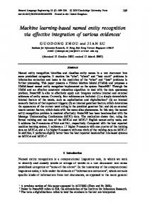
a relativelyissue, complicated as need manytofactors need to consideration. be taken into consideration. For thisofstudy, complicated as manyissue, factors be taken into For this study, most the gas most of the gas sensors are metal oxide (MOX)-based, while the rest are electrochemical-based. The sensors are metal oxide (MOX)-based, while the rest are electrochemical-based. The MOX gas sensor MOX gas sensor is composed of a sensor cap, sensing element and sensor base. Basically, the gas is composed of a sensor cap, sensing element and sensor base. Basically, the gas sensing element is sensing element is coated with a metal oxide—tin dioxide (SnO2)—material that responds to the gas coated with a metal oxide—tin dioxide (SnO2 )—material that responds to the gas molecules, which molecules, which are typically volatile compounds [33]. It consists of two major parts; namely, the are typically volatile compounds [33]. It consists of two major parts; namely, the heater and sensor heater and sensor substrate. The substrate has two terminals, and its resistance is measured as a substrate. The substrate has two terminals, and its resistance is measured as a representation of the representation of the amount of gas concentration in the environment, while the heater provides the amount of gas concentration in the while[34]. the heater the stabilized temperature stabilized temperature needed forenvironment, the measurement Due toprovides its long lifetime, high sensitivity needed for the to its is long lifetime,used high in sensitivity response and lowsuch cost,asthis response andmeasurement low cost, this [34]. type Due of sensor commonly many indoor applications type of sensor is commonly used in many indoor applications such as homes, offices and homes, offices and factories appliances. The second type of gas sensor used in this study factories is the appliances. The secondsensor. type ofThis gastype sensor used has in this is thetoelectrochemical-based electrochemical-based of sensor highstudy sensitivity environmental change sensor. and This typenot of need sensor has high sensitivity to environmental change and it does not needreactants power to it does power to operate. The typical electrochemical sensors consist of chemical operate. The typical sensors anode consistand of chemical (electrolytes or gels) and (electrolytes or gels)electrochemical and two terminals—an a cathode.reactants The anode is responsible for an two terminals—an anode and a cathode. The anode is responsible for an oxidization process and oxidization process and the cathode is responsible for a reduction process. As a result, current isthe createdisby way of positive ions flowing to the As cathode andcurrent the negative ions by flowing to positive the anode. cathode responsible for a reduction process. a result, is created way of ions The output directlyand proportional to the concentration of the sample flowing to theiscathode the negative ions flowing to the anode. Thegases. output is directly proportional The calibration gas sensor to the concentration ofof theeach sample gases. has been carried out in our previous manuscript [35]. For validation, self-developed sensor with the device. manuscript The validation The calibration of each gas nodes sensorwere hasvalidating been carried out commercial in our previous [35]. had been carried out to make that the data with collected by the sensor was similar to the Forprocedure validation, self-developed sensor nodessure were validating the commercial device. The validation data collected by a commercial discussion thiscollected procedure to the NO , procedure had been carried out sensor. to makeThe sure that the of data bywas the limited sensor only was similar to2the temperature and RH sensors. High NO 2 levels in the outdoor environment, originating from local data collected by a commercial sensor. The discussion of this procedure was limited only to the NO2 , traffic or other combustion sources, influences the NO2 level in the indoor environment. Exposure to temperature and RH sensors. High NO2 levels in the outdoor environment, originating from local an excessive level of NO2 could be fatal [4]. The sensor validation was carried out with an Aeroqual traffic or other combustion sources, influences the NO2 level in the indoor environment. Exposure to Ltd.(Auckland, New Zealand) Series 500 portable indoor monitor device (a professional grade air an excessive level of NO2 could be fatal [4]. The sensor validation was carried out with an Aeroqual Ltd. quality measurement system) which had been pre-calibrated [36]. Three sensor nodes and the (Auckland, New Zealand) Series 500 portable indoor monitor device (a professional grade air quality Aeroqual device were placed in a clear, sealed glass container of 100 cm × 40 cm × 30 cm which was measurement system) which had been pre-calibrated [36]. Three sensor nodes and the Aeroqual device completely sealed. Then, the gas concentration inside the sealed container was varied by injecting the were placed in clear, sealed glass container 100 cmwere × 40recorded cm × 30continuously cm which was sealed. particular gasa of interest. The outputs of theof sensors forcompletely 1 h and plotted Then, the 2). gas concentration inside the sealed container was varied by injecting the particular gas of (Figure interest. The outputs of the sensors were recorded continuously for 1 h and plotted (Figure 2).
(a)
(b) Figure 2. Cont.
Appl. 2017, 823 Appl. Sci.Sci. 2017, 7, 7, 823
5 of521 of 21
(c) Figure 2. (a) NO2 data; (b) Temperature data; (c) Humidity data. Figure 2. (a) NO2 data; (b) Temperature data; (c) Humidity data.
Figure showsthe theresult resultof ofthe theNO NO2 sensor sensor when 2 gas concentration was injected Figure 2a2ashows when35 35ppb ppbofofNO NO 2 2 gas concentration was injected to the sealed container. It can be observed that the value for all sensor nodes, thethe Aeroqual to the sealed container. It can be observed that the value for all sensor nodes,including including Aeroqual device, gave relatively similar readings for a one hour period. During the experiment, the same room device, gave relatively similar readings for a one hour period. During the experiment, the same room temperature setting 25 °C was applied as shown in Figure 2b, while Figure 2c shows the readings for temperature setting 25 ◦ C was applied as shown in Figure 2b, while Figure 2c shows the readings for RH. For validation purposes, means and standard deviations for all three parameters were calculated RH. For validation purposes, means and standard deviations for all three parameters were calculated as shown in Table 2 below. Also shown in Table 2, the mean value for NO2, Temp and RH of three as shown in Table 2 below. Also shown in Table 2, the mean value for NO2 , Temp and RH of three nodes nodes (Node 1, Node 2 and Node 3) did not differ substantially from that of Aeroqual (a pre(Node 1, Node 2 and This Nodeshows 3) didthat not the differ substantially from that of Aeroqual (a pre-calibrated device). calibrated device). data measured for each developed sensor modules provide a This shows that the data measured for each developed sensor modules provide a similar response similar response with the pre-calibrated device. On the other hand, the mean value for those three with the pre-calibrated device. On the otherorhand, the mean value for those parameterssuch is within parameters is within an acceptable range exposure limit as suggested by three IAQ authorities as an[10]. acceptable rangedeviation or exposure suggested IAQ [10]. The standard The standard (SD)limit from as Table 2 shows by how the authorities data differedsuch fromasthe mean value for deviation (SD) from Table 2 shows how the data system differedprovides from thereliable mean value each node. Overall, it shows that the developed data. for each node. Overall, it shows that the developed system provides reliable data. Table 2. Means and standard deviations for three parameters. Table 2. Means and standard deviations for three parameters. Node 1 Node 2 Node 3 Aeroqual Parameter Mean SD Mean SD Mean SD Mean SD Node 1 Node 2 Node 3 Aeroqual Parameter NO2 (ppb) (0–80 ppb) 35.9 2.0 34.9 1.7 34.6 1.7 35.5 2.2 Mean 25.6 SD 0.3Mean Temperature (°C) (23–26 °C) 26.5 SD 0.1 Mean 25.7 0.1SD 25.7Mean 0.1 SD Humidity (%) 38–70% 35.9 NO2 (ppb) (0–80 ppb)
39.7 2.0
0.8 34.939.6 1.7 0.6
39.3 34.6
0.61.7 40.235.50.1
2.2
Temperature (◦ C) (23–26 ◦ C)
25.6
0.3
26.5
0.1
25.7
0.1
25.7
0.1
Humidity (%) 38–70%
39.7
0.8
39.6
0.6
39.3
0.6
40.2
0.1
3. Methodology
3.1. Sources of Indoor Air Pollution 3. Methodology Higher IAP levels could lead to certain health effects, while extremely high IAP levels could be fatal. Different IAP Air parameters 3.1. Sources of Indoor Pollutionmay come from different sources and impose different health effects towards humans, as shown in Table 3. Table 3 shows that there are certainly a lot of activities and Higher IAP levels could leadIAP, to certain effects, while extremely high IAP levels could be conditions which could trigger such ashealth air fresheners, combustion appliances, water damage, fatal. Different IAP parameters may come from different sources and impose different health cigarettes, fire and combustion equipment [10,12,13]. However, for the purpose of this study, effects the towards aslimited showntoinfive Table 3. Tableonly, 3 shows thatthey there certainlypresent a lot ofinactivities and sourceshumans, of IAP are conditions because areare commonly the indoor conditions which could air, trigger IAP, such as air the fresheners, appliances, damage, environment: ambient combustion activity, presencecombustion of chemical products, thewater presence of cigarettes, and combustion equipment [10,12,13]. However, for condition the purpose of thisofstudy, food and fire beverages, and the presence of fragrances [17,37–39]. The first of sources indoorthe air pollution is the ambient air.conditions Ambient air refers to thethey air that normally exists in in thethe indoor sources of IAP are limited to five only, because are commonly present indoor environmentambient withoutair, thecombustion presence of other sources of indoorofair pollution. Ambientthe airpresence could pollute environment: activity, the presence chemical products, of food thebeverages, indoor air and if it the carries excessive dust from [17,37–39]. carpets andThe furniture or if it carries too much ozone air and presence of fragrances first condition of sources of indoor from office machines [17]. The second condition of sources of IAP is combustion activity. Combustion pollution is the ambient air. Ambient air refers to the air that normally exists in the indoor environment activities as smoking cigarettes burningair fire-wood release poisonous gasespollute such as the CO indoor and without thesuch presence of other sourcesand of indoor pollution. Ambient air could CO 2, and PM at a higher concentration than ambient air does, which could harm human’s health air if it carries excessive dust from carpets and furniture or if it carries too much ozone from office [37,39]. For theThe purpose of condition this study,of cigarette has been chosenactivity. as the proxy for combustion machines [17]. second sourcessmoking of IAP is combustion Combustion activities
such as smoking cigarettes and burning fire-wood release poisonous gases such as CO and CO2, and PM at a higher concentration than ambient air does, which could harm human’s health [37,39].
Appl. Sci. 2017, 7, 823
6 of 21
For the purpose of this study, cigarette smoking has been chosen as the proxy for combustion activities. The third condition of sources of indoor air pollution is the presence of chemical products or substances. Chemical products such as chemical cleaning agents which are usually used in homes and offices may release VOCs at a poisonous level. Excessive level of VOCs may lead to respiratory-related diseases, such as lung cancer [17]. Thus, for the purpose of this study, chemical cleaning products will be used as the proxy for the presence of chemicals. The fourth condition for sources of indoor air pollution is the presence of food and beverages. Cooking activity or certain food and beverages emit VOCs which could lead to an uncomfortable smell inside a building [38]. VOCs are known to have led to eye irritation, headache and nausea in certain people. Therefore, rotten cooked fish, which has a strong smell and a high level of VOCs, is chosen as the proxy to food and beverages. Table 3. Indoor air pollution (IAP) parameters, its sources and health effects to humans. IAP Pollutant
Sources
Health Effects
O3
Electric arcing, electronic air cleaners, some copiers, and printers
At lower concentration can cause chest pain, coughing, shortness of breath (asthma) and throat irritation
VOC
Air fresheners, furniture, office equipment, cleaning agents
Nausea, damage to the liver, mucous membrane annoyance and asthma
CO
Combustion equipment, engines, faulty heating systems
Fatigues in healthy, chest pain and sore eyes (low concentration) Impaired vision and headaches
NO2
Combustion, gas stoves, water heaters, gas-fired dryers, cigarettes, engines
Cause a variety of pathological changes including the destruction of cilia lining respiratory airways
CO2
Combustion appliances, humans present in room
Cause occupants to grow drowsy and get headaches, shortness of breath
PM10
Stoves, fireplaces, cigarettes, aerosol sprays, cooking
Eye irritation effects and respiratory illness like lung cancer
O2
Photosynthesis from organisms like plants
Nausea, vomiting and lethargic movements
Air conditioning, fire, outdoor air temperature
Hyperthermia, skin pain and can cause serious cardiac arrhythmia
Unsanitary conditions and water damage
Cold and dry will cause skin itchiness. Moisture cause cough, eye irritation
Temperature Humidity
Finally, the presence of fragrances is the fifth condition for the sources of indoor air pollution. Fragrances such as air fresheners and perfumes usually deliver a pleasant smell. However, excessive use of perfumes may cause annoyance and headaches to certain people. In addition, air fresheners usually emit a high amount of VOCs, which may cause irritation and discomfort to certain people [17]. For this project, air freshener is used to substitute for the presence of fragrances. Table 4 summarizes the five conditions for the sources of indoor air pollution and their proxies which have been used in this study. Table 4. Sources of indoor air pollutants. Condition
Proxy
Combustion Activity Chemical Present Fragrance Present Food & Beverage Present Ambient Air
Cigarette Cleaning Agent Air Freshness Rotten Cooked Fish Ambient Air
3.2. Experimental Setup and Data Collection Once all the five conditions of sources of indoor air pollution were identified, an experiment simulating the five conditions was set up for data collection purposes. The experiment was conducted
Appl. Sci. 2017, 7, 823
7 of 21
3.2. Experimental Setup and Data Collection Once all the five conditions of sources of indoor air pollution were identified, an experiment Appl. Sci. 2017, 7, 823 7 of 21 simulating the five conditions was set up for data collection purposes. The experiment was conducted in medium-size room of 4.5 m × 2.4 m × 2.6 m located in a concrete building which is equipped with an at aofheight 2.2 m m×from the floor,in asashown inbuilding Figure 3.which The building is located in air-conditioner medium-size room 4.5 m of × 2.4 2.6 m located concrete is equipped with an 100 m away from main of road, which relatively fromintraffic-related pollution. air-conditioner at the a height 2.2 m fromisthe floor, as far shown Figure 3. Theoutdoor buildingair is located 100Inm addition, thethe location of the building is basically in atraffic-related rural area, which eliminated the influence of away from main road, which is relatively far from outdoor air pollution. In addition, urban air pollution the ambient air. Thus, ambient air measured during experiment is not the location of the on building is basically in a the rural area, which eliminated the the influence of urban air highly influenced by the outside air itself. The room a closed environment and sealed by highly using pollution on the ambient air. Thus, the ambient airwas measured during the experiment is not rubber-seal windows. Theair sensor usedenvironment to collect theand data on the indoor air, was influenced by the outside itself. module, The roomwhich was a is closed sealed by using rubber-seal installed up to the right of the walltoofcollect the room withona the 1.1 indoor m height the ground; a windows.hanging The sensor module, which is used the data air, above was installed hanging position theofbreathing zoneafor occupants The sensor module was powered up to theconsidered right of theas wall the room with 1.1the m height above[10]. the ground; a position considered as the using a 7.5zone V adaptor was programmed to send the data to the base station one minute. breathing for theand occupants [10]. The sensor module was powered using a 7.5every V adaptor and was The data collection over station 16 days between 9:00 a.m. p.m. with the room programmed to sendwas the conducted data to the base every one minute. Theand data5:00 collection was conducted ◦ temperature at 22 °C.9:00 After each experiment, the window was opened to purge the indoor as over 16 daysset between a.m. and 5:00 p.m. with the room temperature set at 22 C. Afteraireach well as to allow toopened enter the room. the Since the ambient airasessentially servedair as to a baseline experiment, the outside windowair was to purge indoor air as well to allow outside enter the for the experiment, the pollutants of interest vary each day based on the ambient air room. Since the ambient air essentially servedwould as a baseline for the experiment, the outside pollutants of interest concentrations thatday day. Sinceonthe essentially served as a baseline forSince the experiment, would vary each based theambient outsideair ambient air concentrations that day. the ambientthe air pollutants interestaswould vary for each day based on the ambient air concentrations essentiallyofserved a baseline the experiment, theoutside pollutants of interest would varythat eachday. day This can beambient accounted for by usingthat dataday. pre-processing such as basedvariation on the outside air concentrations This variationtechniques can be accounted forbaseline by using manipulation. Baseline manipulation the solution to the Baseline problemmanipulation and the correct of data pre-processing techniques such as is baseline manipulation. is the way solution representing the and signal theway analysis deals with the sensor values from units. to the problem thewhen correct of representing signal when thedifferent analysis conversion deals with sensor Baseline manipulation helps to pre-process the sensor output to freetoitself from thethe drift effect, the values from different conversion units. Baseline manipulation helps pre-process sensor output intensity dependence non-linearity [40,41]. detailsfrom aboutnon-linearity other type of[40,41]. data to free itself from the and, drift possibly, effect, thefrom intensity dependence and,The possibly, pre-processing techniques will described in the next section. will be described in the next section. The details about other type ofbe data pre-processing techniques
Figure 3. Room setup for the experiment. Figure 3. Room setup for the experiment.
The process of data collection began with the first condition, which was the ambient air The process of data collection began with the first condition, which was the ambient air environment. The purpose of this experiment was to collect the data of clean air for the room with the environment. The purpose of this experiment was to collect the data of clean air for the room with assumption that the ambient air was not contaminated. For the first environment, the data collection the assumption that the ambient air was not contaminated. For the first environment, the data process took about two days. Thus, at the end of day 2, there were 960 samples collected for ambient collection process took about two days. Thus, at the end of day 2, there were 960 samples collected air. The second environment was the environment with the presence of chemical substance. In this for ambient air. The second environment was the environment with the presence of chemical experiment, a cleaning agent was used as a proxy of the chemical substance. About 100 mL of chemical substance. In this experiment, a cleaning agent was used as a proxy of the chemical substance. About was put in a beaker and placed inside the room—at the centre of the room. The experiment was repeated for two days and 960 samples were collected during that period. For the third environment, an air freshener was used as a proxy for the fragrance. An automatic air freshener which released
Appl. Sci. 2017, 7, 823
8 of 21
Appl. Sci. 2017, 7, 823
8 of 21
100 mL of chemical was put in a beaker and placed inside the room—at the centre of the room. The experiment was repeated for two days and 960 samples were collected during that period. For the third environment, anwas air freshener was used as a proxy forhung the fragrance. Anadjacent automatic air freshener fragrance every 15 min placed inside the room. It was on the wall to the wall where released fragrance every 15 min inside the room.2 It hung the wall adjacent thewhich sensing node was placed, about 2 m was fromplaced the floor and about mwas from the on sensing node. The air to the wall where the sensing node was placed, about 2 m from the floor and about 2 m from the flow from the air conditioner would accumulate the fragrance in the room. The data was collected sensing node. The air flow from the air conditioner would accumulate the fragrance in the room. The for two days with 960 samples. For the fourth condition of the room environment with combustion data was collected for two adays with 960 samples. of the environment activity, a person smoking cigarette was chosenFor as the thefourth proxy.condition A person wasroom asked to smoke in with combustion activity, a person smoking a cigarette was chosen as the proxy. A person was asked the room so that the real data of a person smoking a cigarette in a room was collected. That person to smoke in the room so that the real data of a person smoking a cigarette in a room was collected. smoked one cigarette at the centre of the room. Every cigarette produced data for approximately That person smoked one cigarette at the centre of the room. Every cigarette produced data for 30 min. The experiment was repeated four times a day for eight days. The amount of data collected for approximately 30 min. The experiment was repeated four times a day for eight days. The amount of the environment with combustion activity was 960 samples. Lastly, for the room environment with data collected for the environment with combustion activity was 960 samples. Lastly, for the room the presence of food and beverages, rotten cooked fish had been selected to represent this category. environment with the presence of food and beverages, rotten cooked fish had been selected to A bowl of rotten cooked fish was placed in the middle theplaced room. in The experiment repeated represent this category. A bowl of rotten cooked fishofwas the middle of was the room. Thefor two days and 960 samples were collected during that period. experiment was repeated for two days and 960 samples were collected during that period.
3.3.3.3. Sensor Response Sensor Response In In this section, five different differentconditions conditionsofofsources sources indoor this section,the thesensors’ sensors’response response towards towards the the five ofof indoor airair pollution—ambient air, combustion activity, chemical presence, fragrance product (air freshener) pollution—ambient air, combustion activity, chemical presence, fragrance product (air freshener) and foods and fish)—isdiscussed. discussed.Figure Figure shows that sensors and foods andbeverages beverages(rotten (rotten cooked cooked fish)—is 4a4a shows that thethe sensors gavegave a a relatively thetime. time.The Thesensors’ sensors’response responsewas wasasasexpected expected there was relatively steady steady reading reading throughout throughout the asas there was nono substance which concentration.On Onthe theother other hand, Figure substance whichcould couldinterrupt interruptthe the ambient ambient air concentration. hand, in in Figure 4b,4b, with thethe presence ofofa achemical bychemical chemicalcleaning cleaning product, it can with presence chemicalsubstance, substance,which which is represented represented by product, it can observed that certaingas gassensors, sensors,such such as as VOCs, VOCs, NO22 and to to be be observed that certain and O O33, ,reacted reacteddifferently differentlycompared compared ambient environment.The Thereading reading of of the the VOCs VOCs gas when thethe ambient environment. gas sensor, sensor, particularly, particularly,raised raisedsharply sharply when chemical was present room. A similar situation could observed with presence food chemical was present in in thethe room. A similar situation could bebe observed with thethe presence ofof food and and beverages, was represented by rotten cooked as shown in Figure 4c. graph The graph for beverages, which which was represented by rotten cooked fish asfish shown in Figure 4c. The for VOCs VOCs increased dramatically first introduced then remained at the increased dramatically when thewhen smellthe wassmell first was introduced and thenand remained at the peak. Thepeak. graph The graph for other gases did not change much. Notably, in all graphs, a different set of gas sensors for other gases did not change much. Notably, in all graphs, a different set of gas sensors reacted reacted differently towardsconditions. different conditions. In thesections, following raw data collected differently towards different In the following thesections, raw datathe collected went through went through pattern recognition procedures. Figure 4d represents the response of the sensors when pattern recognition procedures. Figure 4d represents the response of the sensors when the automatic the automatic air freshener released fragrance into the room every 15 min. The fragrance of the air air freshener released fragrance into the room every 15 min. The fragrance of the air freshener however, freshener however, vaporized quickly into the air after it was released. Thus, these changes of high vaporized quickly into the air after it was released. Thus, these changes of high and low concentration and low concentration of fragrance in the air could be observed from the disturbed graph. of fragrance in the air could be observed from the disturbed graph.
(a)
(b) Figure 4. Cont.
Appl. Sci. 2017, 7, 823 Appl. Sci. 2017, 7, 823 Appl. Sci. 2017, 7, 823
9 of 21 9 of 21 9 of 21
(c) (c)
(d) (d)
(e) (e) Figure 4. (a) Ambient environment; (b) Chemical presence; (c) Food and beverages; (d) Fragrance Figure 4. 4. (a)(a) Ambient (c) Food Foodand andbeverages; beverages;(d)(d)Fragrance Fragrance Figure Ambientenvironment; environment; (b) (b) Chemical Chemical presence; presence; (c) presence; and (e) Combustion activity. presence; and (e)(e) Combustion presence; and Combustionactivity. activity.
Meanwhile, for the last condition, 30 min of data were recorded instead of 8 h because the effects Meanwhile, thelast last condition,30 30min min of of data data were recorded instead ofof8 8h hbecause thethe effects Meanwhile, forfor the werethe recorded because effects of cigarette smoke only last condition, for 30 min. Figure 4e illustrates effect ofinstead the cigarette smoking activity of cigarette smoke onlylast lastfor for30 30min. min.Figure Figure 4e 4e illustrates the effect ofofthe cigarette smoking activity of on cigarette smoke only illustrates the effect the cigarette smoking activity the sensor in the room. Notably, in all graphs, a different set of gas sensors reacted differently on sensor theroom. room.Notably, Notably, in in all all graphs, graphs, aa different differently ontowards thethe sensor ininthe different set setof ofgas gassensors sensorsreacted reacted differently different conditions. towards different conditions. towards different conditions. 3.4. Steps in Pattern Recognition Steps PatternRecognition Recognition 3.4.3.4. Steps in in Pattern The multivariate response of an array of chemical gases with broad and partially overlapping The multivariateresponse responseofofan anarray array of of chemical chemical gases with broad and overlapping The multivariate gases of with broad andpartially partially overlapping selectivity created “electronic fingerprints” for a wide range odour which can be characterized selectivity created “electronic fingerprints” for a wide range of odour which can be characterized using pattern-recognition. process of pattern recognition be split into four stages: selectivity created “electronicThe fingerprints” for a wide range ofmay odour which can be sequential characterized using using pattern-recognition. The process of pattern recognition may be split into four sequential stages: data pre-processing, dimensionality reduction, classification and decision making. Figure 5 illustrates pattern-recognition. The process of pattern recognition may be split into four sequential stages: data data pre-processing, dimensionality reduction, classification and decision making. Figure 5 illustrates the pattern recognition process.reduction, Each stageclassification is described in detail in themaking. followingFigure sections. pre-processing, dimensionality and decision 5 illustrates the the pattern recognition process. Each stage is described in detail in the following sections. pattern recognition process. Each stage is described in detail in the following sections.
Sensor Sensor Response Response
Data Data Preprocessing Preprocessing
Classification Dimensionality Classification Dimensionality Network Reduction Network Reduction Optimization Feedback Optimization Feedback
Figure 5. 5. Steps Steps in Figure in pattern patternrecognition. recognition. Figure 5. Steps in pattern recognition.
Decision Decision Making Making
Appl. Sci. 2017, 7, 823 Appl. Sci. 2017, 7, 823
10 of 21 10 of 21
The first first stage stage of of the the pattern pattern recognition process, after after collecting collecting raw raw data, The recognition process, data, is is data data pre-processing. pre-processing. Data pre-processing is a procedure that involves extracting certain significant characteristics from the the Data pre-processing is a procedure that involves extracting certain significant characteristics from sensor response response curves curves or or transient transient response response in in order order to to produce produce aa set set of of numerical numerical data data or or feature feature sensor for further processing [42]. Choosing the correct pre-processing technique is important because for further processing [42]. Choosing the correct pre-processing technique is important because itit may aid aid in in the the success success of of subsequent subsequent analysis analysis and and affect affect the the performance performance of of pattern pattern recognition recognition [43]. [43]. may Most data datapre-processing pre-processingtechniques techniquesare arebasically basicallyderived derived from a typical sensor response as shown Most from a typical sensor response as shown in in Figure 6. Vo is a measured value in clean ambient air or an initial value called the baseline, Figure 6. Vo is a measured value in clean ambient air or an initial value called the baseline, whilewhile Vs is Vs is the response to odour or smell. the response value value to odour or smell.
Figure 6. 6. Typical Typical sensor sensorresponse. response. Figure
Basically, Basically, data data pre-processing pre-processing techniques techniques can can be be divided divided into intothree threemajor majorcategories: categories: baseline baseline manipulation, manipulation, normalization normalization and and compression. compression. Every category has their own own formula formula which which was was transformed response. In In thisthis study, onlyonly fivefive datadata pre-processing techniques have been transformedfrom fromthe thesensor sensor response. study, pre-processing techniques have selected whichwhich are frequently used in odour pattern recognition as summarized in Table 5. These five been selected are frequently used in odour pattern recognition as summarized in Table 5. These techniques, calledcalled features of pattern recognition and raw data, alsoare chosen one ofasthe features. five techniques, features of pattern recognition and raware data, also as chosen one of the The feature output from the pre-processing stage are often notare suitable to besuitable processed byprocessed the classifier features. The feature output from the pre-processing stage often not to be by due data redundancy andredundancy high-dimensionality that can cause thethat problem dimensionality [44]. the to classifier due to data and high-dimensionality can of cause the problem of On the other hand, toothe many features are used forfeatures the classification, there a risk that the model dimensionality [44].ifOn other hand, if too many are used for the is classification, there is a becomes too model complex and the of the to classify be to very poor.can Forbethis reason, risk that the becomes toocapability complex and themodel capability of the can model classify very poor. aFor dimensionality stage is requiredstage to eliminate the curse of dimensionality classification this reason, areduction dimensionality reduction is required to eliminate the curse ofin dimensionality and improve theand accuracy or performance in classification improve the accuracyof orclassification performance[45]. of classification [45]. Table Table5.5. Data Data pre-processing pre-processingtechniques techniquesselected. selected.
Technique Technique Raw Raw Differential Differential Relative Relative Fractional Fractional
Abbreviation Abbreviation RW RW DIFF DIFF REL REL FRACT FRACT
Sensor Normalization Sensor Normalization
SN
SN
Formula Formula = Xij = Vij = − Xij = Vij − Vbj = V Xij = Vbjij − = V −V Xij = ijVbj bj − Vij − Vijmin = Xij = V max− − V min ij
Vector Array Normalization Vector Array Normalization
VAN VAN
Xij ==
References References [46] [46] [43,46,47] [43,46,47]
[43,46,47] [43,46,47]
ij
Vij q
2
N ∑∑q=1((Vij ))
Where, Xij represents feature matrix for the ith sample of jth sensor, Vij represents sensor’s response value, and Vbj represents baseline value of Vij . A feature extraction technique based on principal component analysis (PCA), which is widely used in in machine learning for dimensionality reduction, is chosen for this study [22,48,49]. PCA is
Appl. Sci. 2017, 7, 823
11 of 21
defined by a matrix having as rows the eigenvectors of the feature space covariance matrix. The PCA removes any redundancy between the components of the projected vectors, since the covariance matrix in the transformed space becomes diagonal as shown in Equation (1):
∑ y = diag[λ1 λ2 . . .
(1)
λn ]
where, {λi }i=1...n represent for the eigenvalues of the covariance matrix. The PCA performs the vector projection without any knowledge of their labels. This transformation is defined in such a way that the first principal component has as high a variance as possible and each succeeding component in turn has the highest variance possible under the constraint that it be orthogonal to the preceding components. It is therefore known as an unsupervised data analysis method or algorithm since it “ignores” class labels [50–52]. In this research, PCA was used to remove any redundancy between the components of the projected vectors and reduce the dimension of the original dataset. The result is explained in term of the “total variance explained” table. The table shows the number of the principal component (PC) that has been extracted with eigenvalue and how much information (variance) can be attributed to each component. Only a few components will be selected based on “eigenvalue-one criterion”. In PCA, one of the most commonly-used criteria for solving the number of components problem is the eigenvalue-one criterion, also known as the Kaiser criterion [53]. With this approach, any component with an eigenvalue greater than 1.00 will be selected, and thus it will reduce the dimension of original datasets which have nine dimensions. Table 6 shows the total variance explained for the raw (RW) feature after being analyzed via PCA. The table clearly shows that most of the variance (31.77%) can be explained by the first principal component (PC1) alone. The second principal component (PC2) still bears some information (23.42%) while the third (PC3) and fourth principal components (PC4) bear least information with variance of 14.59% and 11.16%. respectively. Based on “eigenvalue-one criterion”, four components (PC1, PC2, PC3 and PC4) have been selected because they display an eigenvalue greater than 1.00 and hold the greater amount of variance. Together, the selected components explain 80.88% of the information. Table 6. Total variance explained for raw (RW) feature. Initial Eigenvalues PC 1 2 3 4 5 6 7 8 9
Extraction Sums of Squared Loadings
Total
Variance (%)
Cumulative (%)
Total
Variance (%)
Cumulative (%)
2.854 2.108 1.313 1.005 0.833 0.407 0.278 0.152 0.051
31.711 23.420 14.590 11.162 9.251 4.526 3.085 1.685 0.571
31.711 55.131 69.720 80.882 90.133 94.659 97.744 99.429 100.000
2.854 2.108 1.313 1.005
31.711 23.420 14.590 11.162
31.711 55.131 69.720 80.882
The dimensionality reduction based on PCA has also been performed to other features. Table 7 illustrates the overall results for all features. According to Table 7, it is clear that most features can be explained based on four dimensions, except for vector array normalization (VAN), which can be explained by two dimensions only. VAN also gave the highest total variance explained at 93.70%. All other features are being dimensionally reduced from nine dimensions to four dimensions, with differential (DIFF) being the second-highest total variance explained at 84.48%, while SN was the lowest total variance explained at 73.99% only. Other features gave a similar result to raw (RW) at 80.88%, and relative (REL) and fractional (FRACT) shared the same percentage at 80.85%.
Appl. Sci. 2017, 7, 823
12 of 21
Table 7. Total variance explained for all features. Feature
Original Dimension
New Dimension
Total Variance Explained
RW DIFF REL FRACT SN VAN
9 9 9 9 9 9
4 4 4 4 4 2
80.88% 84.48% 80.85% 80.85% 73.99% 93.70%
4. Results and Discussion 4.1. Supervised Machine Learning Analysis for Pattern Recognition There are various supervised machine learning used in classification techniques, which can be sorted into a few categories: logic-based, perceptron-based, instance-based, statistical learning-based and vector-based [54]. The classifiers for each category are shown in Table 8. For this study, three algorithms which have been used in many applications, especially involving odour or smell classification, have been chosen: MLP (perceptron-based), KNN (instance-based), and LDA (statistical learning-based) [55–57]. All of these classifiers have been run using MATLAB’s 2015 functions library that supports supervised machine learning. At the end of the program, the MATLAB R2015b (version 8.6, The MathWorks Company, Natick, MA, USA, 2015) produced an output file which then embedded to the system. Table 8. Methods for supervised machine learning. Method
Classifier
Logic-based
• •
Decisions trees Rule based
Perceptron-based
• •
Artificial neural network (ANN) Multilayer perceptron (MLP)
Instance-based
•
K-nearest neighbour (KNN)
Statistical Learning-based
•
Linear discriminant analysis (LDA)
Vector-based
•
Support vector machine (SVM)
The example of one of the algorithms, such as the MLP model, along with its classification performance of six features is discussed in this section. For each of the features, a separate MLP model was formulated. Separate models need to be formulated as the aim of the research is to find the optimal classification accuracy for each feature. In order to identify the source affecting the IAQ, this study used the MLP, which consists of three layers: the input layer, hidden layer and output layer. As network architecture, a 3-layer perceptron model as shown in Figure 7 was used. The first input layer contains the input variables for the network, which is the data after the pre-processing technique. For the data set before PCA, the input layer contains nine neurons of IAQ parameters, which are CO2 , CO, O3 , NO2 , O2 , VOC, PM10 , temperature and humidity, while, for the data set after PCA, the input layer contains the dimensions for each feature after reduction. There is one hidden layer used and the numbers of hidden neurons were not fixed and were adjusted until the desired performance was achieved. The last layer of the model is the output layer, which consists of five target outputs that represent five types of sources of indoor air pollution, such as combustion activity, the presence of fragrances and so on. Sixty percent of all data is selected randomly to become the training set. A goal is set (in this case, a mean square error (MSE) of 0.0001 has been chosen as the goal)
Appl. Sci. 2017, 7, 823
13 of 21
Appl. Sci. 2017, 7, 823
13 of 21
goal) and thedataset trainingisdataset trained the desired is obtained. MSEused was used the and the training trainedis until theuntil desired MSE isMSE obtained. MSE was as theasstopping stopping criterion. Training was conducted until the MSE fell below 0.0001 or a maximum epoch limit criterion. Training was conducted until the MSE fell below 0.0001 or a maximum epoch limit of 1000 is of 1000 is reached. This is to ensure that the model is trained with minimum error iteration and not reached. This is to ensure that the model is trained with minimum error iteration and not over-trained. over-trained. The learning rate and momentum factor were chosen based on experimental analysis. The learning rate and momentum factor were chosen based on experimental analysis. The number of The number of hidden neurons was adjusted by the network to achieve this goal. The testing hidden neurons adjusted by themodel network achieve thisThis goal.value The is testing toleranceallowable of the neural tolerance of was the neural network was to chosen as 0.1. the maximum network model was as 0.1. This value is the maximum allowable tolerance level for the testing. tolerance level forchosen the testing.
Figure 7. Network architecture of the multilayer perceptron (MLP) model. Figure 7. Network architecture of the multilayer perceptron (MLP) model.
The The detailed parameter forforMLP givenininTable Table9.9.For For example, to train the dataset detailed parameter MLPtraining training is is given example, to train the dataset (before PCA) for the condition ofofambient datafrom fromall all9 9IAQ IAQ parameters become the neurons (before PCA) for the condition ambientair, air,the the data parameters become the neurons for the input layer. Randomly, 60% of each IAQ parameter was selected to be the training set (60% out for the input layer. Randomly, 60% of each IAQ parameter was selected to be the training set (60% of 960 fordata ambient air). air). TheThe training was untilthe thetargeted targeted MSE reached outdata of 960 for ambient training wasconducted conducted until MSE waswas reached or or a maximum epoch limit 1000was wasreached. reached. This was repeated withwith the other four four untiluntil a maximum epoch limit ofof1000 Thisprocess process was repeated the other conditions. In the end, networkwould would produce produce aamodel was then tested against the 40% conditions. In the end, thethe network modelwhich which was then tested against the 40% of the remaining data for all conditions (the testing set) in order to find the classification accuracy. of the remaining data for all conditions (the testing set) in order to find the classification accuracy. The whole process was repeated again for different features. The model of the feature that gave the The whole process was repeated again for different features. The model of the feature that gave the highest classification accuracy may be chosen to be embedded into the system after being compared highest classification accuracy may be chosen to be embedded into the system after being compared to to the model of other type of classifiers, such as KNN or LDA. the model of other type of classifiers, such as KNN or LDA. Table 9. Parameters for multilayer perceptron (MLP) training.
Table 9. Parameters for multilayer perceptron (MLP) training.
• •
Training Parameter Value Sample Training Parameter Value • Number of samples used for training: 2880 4800 • Number of samples Sampleused for testing: 1920 Input 9 4800 Number of samples used for training: 2880 Hidden used neurons Number of samples for testing: 1920 Flexible Output neurons 5 Input Performance MSE 9 HiddenGoal neurons Flexible 0.0001 Output neurons Learning rate 0.01 5 Performance Momentum constant 0.5MSE
Goal Learning rate Momentum constant
0.0001 0.01 0.5
Appl. Appl. Sci. Sci. 2017, 2017, 7, 7, 823 823
14 14 of of 21 21
The classification performance of the MLP, KNN and LDA using the six features for the dataset The classification performance of the MLP, KNN LDA the six because features PCA for the before-PCA and after-PCA are shown in Figure 8. Theand PCA wasusing performed is dataset known before-PCA and after-PCA are shown in Figure 8. The PCA was performed because PCA is known to to be able to increase the classification accuracy of certain datasets by reducing the number of be able to losing increase theaclassification of[46]. certain datasetsasby reducing the number of variables, variables, only minimum of accuracy variability However, shown in Figure 8, the classification losing a minimum ofisvariability [46].classification However, asrate shown in Figure 8, all thefeatures. classification rate for rate foronly dataset after PCA less than the before PCA for This result is dataset after PCA is less than the classification rate before PCA for all features. This result is due to due to the information loss during PCA. According to [58], for datasets with very low complexity the information loss during PCA. According [58], forduring datasets with very of low complexity (few PCs), (few PCs), the relevant information has been to excluded the process PCA, which resulted in relevant information has been during theThe process PCA,give which resulted in a lower athe lower classification accuracy for excluded datasets after PCA. PCAofcould a higher classification classification accuracy for very datasets PCA. The PCAPCs), couldwhere give athe higher classification accuracy to accuracy to datasets with highafter complexity (many dataset before PCA does not datasets very information, high complexity (many PCs), noise where[59]. the With dataset PCA have only havewith relevant but also contains thebefore presence of does noise,not theonly classifier relevant the information, but and also thus contains [59]. Withwell. the presence noise, the classifier over-fits over-fits training data doesnoise not generalize Based onofthe explanation by [58], it can theseen training datastudy and thus not generalize Based on the explanation by [58], can process be seen be that this has adoes dataset with a verywell. low complexity (only 9 PCs). Thus, theitPCA that excluded this studyrelevant has a dataset with athat verycould low complexity (only PCs). Thus, the PCA process has has information contribute to the 9high classification accuracy, which excluded relevant information that could contribute to the high classification accuracy, which explains explains the lower classification accuracy for the dataset after PCA. Nevertheless, although the the lower classification for thenot dataset after classification PCA. Nevertheless, although dataset after dataset after PCA (VANaccuracy feature) could give 100% accuracy, it couldthe classify 99.58% PCA feature) not variables give 100%instead classification could classify 99.58% of the dataset of the(VAN dataset using could only two of nineaccuracy, variablesitneeded for the dataset before PCA. using only two variables instead of nine variables needed for the dataset before PCA.
Classification before PCA Classification Accuracy (%)
100.00 90.00 80.00 70.00 60.00 RW DIFF REL
FRA CT
SN
VAN
MLP 99.69 98.33 97.92 97.81 89.69 100.0 KNN 99.06 98.96 98.13 98.13 97.50 100.0 LDA 97.60 96.56 95.73 95.73 85.10 99.38
Classification Accuracy (%)
Classification after PCA 100.00 90.00 80.00 70.00 60.00 RW
DIFF
REL
FRA CT
SN
VAN
MLP 96.67 97.50 97.29 97.29 70.00 99.58 KNN 98.44 98.75 98.02 98.02 88.33 97.92 LDA 92.19 93.96 94.69 94.69 64.17 66.56
Figure 8. Classification Classification performance performance for for the the beforebefore- principal principal component component analysis analysis (PCA) (PCA) and and afterafterprincipal component analysis (PCA) dataset.
The validation in identifying pollutants pollutants by the proposed machine learning algorithm can be confusion matrix. A confusion matrix is a table is often to describe obtained by bylooking lookingatatthethe confusion matrix. A confusion matrix is a that table that isused often used to the performance of a classification model (or model “classifier”) on a set of on testadata fortest which values describe the performance of a classification (or “classifier”) set of datathe fortrue which the are known. For example, in the case of the MLP classifier, the confusion matrix for the features giving true values are known. For example, in the case of the MLP classifier, the confusion matrix for the the lowest and the lowest highestand classification are shown in Tables 10 and 11. Rows and 11. columns features giving the highestaccuracy classification accuracy are shown in Tables 10 and Rows represent actual and predicted respectively. Tablerespectively. 10 shows the Table confusion matrix the for feature SN and columns represent actualvalues, and predicted values, 10 shows confusion (after PCA) as it gave the lowest matrix. Based on the matrix. table, itBased can beon observed that every matrix for feature SN (after PCA)confusion as it gave the lowest confusion the table, it can be condition contributes to the confusion level, with activity having highest confusion levelthe at observed that every condition contributes to thehuman confusion level, withthe human activity having 50%. This means that MLP can classify only 50% of combustion activity correctly and it cannot classify highest confusion level at 50%. This means that MLP can classify only 50% of combustion activity the other and 50%itcorrectly as combustion activity. correctly cannot classify the other 50% correctly as combustion activity. thethe confusion matrix for VAN which has which the highest Table 1111presents presents confusion matrix for(before VAN PCA) (before PCA) has classification the highest accuracy. Compared to the confusion matrix of SN in Table 10, MLP does not have any classification accuracy. Compared to the confusion matrix of SN in Table 10, MLP does notconfusion have any in classifying all the fiveall conditions. It means that it canthat classify of the all fiveofconditions correctly. confusion in classifying the five conditions. It means it canallclassify the five conditions This confusion matrix validates the classification rate for VAN PCA), which is 100%. correctly. This confusion matrix validates the classification rate (before for VAN (before PCA), which is 100%.
Appl. Sci. 2017, 7, 823
15 of 21
Table 10. Confusion matrix of multilayer perceptron (MLP) for sensor normalization (SN) after principal component analysis (PCA). Predicted
Actual
Sources of IAQ Pollutant
Ambient
Chemical
Food & Beverages
Fragrance
Human Activity
Confusion Level (%)
Ambient Chemical Food & Beverages Fragrance Human Activity
276 16 0 6 4
88 308 16 16 12
20 50 280 40 60
0 10 84 288 116
0 0 4 34 192
28.13 19.79 27.08 25.00 50.00
Table 11. Confusion matrix of multilayer perceptron (MLP) for vector array normalization (VAN) before principal component analysis (PCA). Predicted
Actual
Sources of IAQ Pollutant
Ambient
Chemical
Food & Beverages
Fragrance
Human Activity
Confusion Level (%)
Ambient Chemical Food & Beverages Fragrance Human Activity
384 0 0 0 0
0 384 0 0 0
0 0 384 0 0
0 0 0 384 0
0 0 0 0 384
0 0 0 0 0
The classification accuracy that has been achieved by this study is quite similar to the classification result achieved by a previous researcher [46]. They have developed a laboratory-made malodour sensing system, used to identify five typical sources of olfactive annoyance: printing houses, a paint shop in a coach building, wastewater treatment plant, urban waste composting facilities and a rendering plant. The researcher adopted various data pre-processing techniques, such as the VAN feature, which was also used in this study. Their results also show that the best classification results are obtained using a VAN feature with 100% classification accuracy. The objective of testing these three classifiers is to see which classifier gives the highest classification accuracy. Based on the results of the classifiers discussed before, there are four sets of classifiers with one feature (VAN before PCA) which gave 100% classification accuracy: (1). (2). (3). (4).
MLP-VAN feature before PCA (model 9-3-5), MLP-VAN feature before PCA (model 9-9-5), MLP-VAN feature before PCA (model 9-12-5), and KNN-VAN feature before PCA (K factor is 2).
To prove that the VAN feature before PCA really gave 100% classification accuracy, another analysis has been done. The PCA visualization for the VAN feature before any dimensionality reduction is constructed in s 3D plot as shown in Figure 9. From Figure 9, it can be seen that none of the five conditions coincide with each other, and therefore they are mutually exclusive. After the feature has been identified, it is now time to choose between the two classifiers: MLP or KNN. This study chooses MLP with a model structure of 9-3-5 because it is easier to be embedded in the system. Model 9-3-5 only has three hidden variables, while the other two model structures have nine and 12 hidden variables. A model structure with fewer hidden variables has a less complicated formula and is therefore easy to be embedded. As far as KNN is concerned, KNN requires a large storage space in the system because it saves every data that it receives. MLP, on the other hand, does not require a large storage system. Due to these reasons, an MLP classifier is chosen for this study.
Appl.Appl. Sci. 2017, 7, 8237, 823 Sci. 2017,
16 of 16 21 of 21
Figure 9. 3D plot of PCA visualization for the VAN feature. Figure 9. 3D plot of PCA visualization for the VAN feature.
4.2. Classification of Multiple Sources of IAP 4.2. Classification of Multiple Sources of IAP This section shows results for the classification of sources of IAP when multiple sources are This section shows results for the classification of sources of IAP when multiple sources are present present at the same time. Based on the previous result, the MLP classifier with a model structure of at the same time. Based on the previous result, the MLP classifier with a model structure of 9-3-5 was 9-3-5 was chosen for this analysis. To collect the related data for this analysis, an experiment that chosen for this analysis. To collect the related data for this analysis, an experiment that simulates the simulates the presence of multiple sources of IAP was conducted. A similar environment to the presence of multiple sources of IAP was conducted. A similar environment to the previous experiment previous experiment of collecting a single source of IAP was maintained, where the sensor module of collecting a single source of IAP was maintained, where the sensor module was installed hanging was installed hanging up to the right of the wall with 1.1 m of height above the ground, and the up to the right of the wall with 1.1 m of height above the ground, and the temperature of the room was temperature ◦of the room was set to 22 °C. The data was collected for one day: between 9:00 a.m. and set to 22 C. The data was collected for one day: between 9:00 a.m. and 11:30 a.m. Figure 10 shows the 11:30 a.m. Figure 10 shows the process of data collection for testing the system when all sources process of data collection for testing the system when all sources present in a room. present in a room. The experiment began with the first condition present, which was the ambient air. There were The experiment began with the first condition present, which was the ambient air. There were 45 samples collected for ambient air over 45 min duration. This environment was tagged as “single 45 samples collected for ambient air over 45 min duration. This environment was tagged as “single source”. Then, an automatic air freshener which released fragrance every 15 min was placed inside source”. Then, an automatic air freshener which released fragrance every 15 min was placed inside the room. This environment was conducted to simulate the presence of two sources: ambient air and the room. This environment was conducted to simulate the presence of two sources: ambient air and fragrance. The air freshener was hung up on the wall with a height of 2 m from the floor and about 2 m fragrance. The air freshener was hung up on the wall with a height of 2 m from the floor and about 2 from the sensing node. Total data collected for the air freshener was over 75 min. This environment is m from the sensing node. Total data collected for the air freshener was over 75 min. This environment tagged as “mixed sources A”. After that, a person was asked to smoke in the room. This environment is tagged as “mixed sources A”. After that, a person was asked to smoke in the room. This was conducted to simulate the presence of three sources of IAP: ambient air, fragrance and single environment was conducted to simulate the presence of three sources of IAP: ambient air, fragrance cigarette smoke. That person smoked one cigarette at the centre of the room. One cigarette took 10 min, and single cigarette smoke. That person smoked one cigarette at the centre of the room. One cigarette which contribute to a 10 min data sample. This environment was tagged as “mixed sources B”. Lastly, took 10 min, which contribute to a 10 min data sample. This environment was tagged as “mixed the other two sources of IAQ, which are food and beverages and chemical cleaning product, were sources B”. Lastly, the other two sources of IAQ, which are food and beverages and chemical cleaning added into the environment. These two sources of IAP were placed in the middle of the room for product, were added into the environment. These two sources of IAP were placed in the middle of 20 min, which gave 20 samples. This environment was conducted to simulate the presence of all the room for 20 min, which gave 20 samples. This environment was conducted to simulate the five sources of IAP. Although there was no person smoking in the room at this time, the presence of presence of all five sources of IAP. Although there was no person smoking in the room at this time, smoking can still be traced. The presence of smoking can be traced up to 30 min, as shown in Figure 10. the presence of smoking can still be traced. The presence of smoking can be traced up to 30 min, as This environment was tagged as “mixed sources C”. shown in Figure 10. This environment was tagged as “mixed sources C”.
Appl. Sci. 2017, 7, 823
17 of 21
Appl. Sci. 2017, 7, 823
17 of 21
Experiment Setting
Single Source •
Duration
= 9.00 to 9.45am
•
IAP Source
= Clean air
•
1 minute
= 1 sample
•
Data Collected
= 45 samples
Mixed Sources A •
Day
•
IAP Source
= Clean air + Air freshener
•
1 minute
= 1 sample
•
Data Collected
= 75 samples
•
Day
= 11.01 to 11.10am
•
IAP Source
= Clean air + Air freshener + Cigarette smoke
•
1 minute
= 1 sample
•
Data Collected
= 10 samples
•
Day
•
IAP Source
= Clean air + Air freshener + Cigarette smoke
•
1 minute
= 1 sample
•
Data Collected
= 9.46 to 11.00am
Mixed Sources B
Mixed Sources C = 11.11 to 11.30am +Rotten Cooked Fish + Cleaning Agent = 20 samples
Figure Data collectionprocedures procedures for present. Figure 10.10. Data collection formultiple multiplesources sources present.
Figure 11 shows resultofofthe thesensor’s sensor’s response allall situations as described above,above, from afrom Figure 11 shows thethe result responseforfor situations as described single source fivesources sources of of IAP. IAP. It It can can be sensors react differently whenwhen a single source upup totofive be observed observedthat thatthe the sensors react differently additional sources of IAP are added into the room. The result of the classifier based on all additional sources of IAP are added into the room. The result of the classifier based on all environments environments is shows in Table 12. Based on the table, it can be observed that the system can precisely is shows in Table 12. Based on the table, it can be observed that the system can precisely detect a single detect a single source (ambient) with 45 correct classifications out of 45 data samples. This means that source (ambient) with 45 correct classifications out of 45 data samples. This means that the MLP the MLP classifier can classify an ambient environment at 100% classification rate. Similarly, when classifier can classify an ambient environment at 100% classification rate. Similarly, when the the fragrance is present in the condition of “mixed sources A”, the system correctly classifies thefragrance two is present in the condition of “mixed sources A”, the system correctly classifies the two mixed sources mixed sources of IAQ. The system did not misclassify the sources as unknown sources. This result is of IAQ. as Theexpected system did not misclassify the sources as unknown result expected because because the environment of fragrance mixed sources. with the This ambient airisisassimilar to the the environment of fragrance with the has ambient airbeen is similar the such presence of fragrance presence of fragrance alone,mixed and the system already trainedtowith an environment. Onalone, the system other hand, systembeen could not classify samples out of 10 samples as the available and the hasthe already trained withtwo such an environment. On the other hand,sources the system air, presence of fragrance and smoke) in the condition of “mixed could(ambient not classify two samples out of 10presence samplescigarette as the available sources (ambient air, sources presence of B”. Nonetheless, the MLP classifier correctly classified the other eight samples as fragrance (one) the and MLP fragrance and presence cigarette smoke) in the condition of “mixed sources B”. Nonetheless, cigarette smoke (seven). The result is also as expected, because the presence of smoking was classifier correctly classified the other eight samples as fragrance (one) and cigarette smoke (seven). overpowering the presence of fragrance due to the high amount of gases produced during smoking The result is also as expected, because the presence of smoking was overpowering the presence of fragrance due to the high amount of gases produced during smoking as compared to the amount of gases produced by air freshener. Likewise, in the condition of “mixed sources C”, when all of the sources of IAP were mixed together in the room, the MLP classifier could correctly classify 50% of
Appl. Sci. 2017, 7, 823
18 of 21
Appl. Sci. 2017, 7, 823
18 of 21
as compared to the amount of gases produced by air freshener. Likewise, in the condition of “mixed sources C”, when all of the sources of IAP were mixed together in the room, the MLP classifier could the samples combustion (one),asfood and beverages of chemical (seven). correctlyasclassify 50% ofactivity the samples combustion activity (two) (one), and foodpresence and beverages (two) and The other 10 samples have been classified as unknown sources. presence of chemical (seven). The other 10 samples have been classified as unknown sources.
Mixed
Single Source
Sources A
Mixed
Mixed
Sources B Sources C
Figure Sensor’s responsewhen when additional additional sources IAP areare present. Figure 11. 11. Sensor’s response sourcesofof IAP present. Table 12. Result of the classifier based on mixed sources.
Table 12. Result of the classifier based on mixed sources. Data Condition Samples Data Samples Condition Single source SingleMixed sourcesources A Mixed sources A Mixed sources B Mixed Mixed sourcessources B C Mixed sources C
45 75 10 20
45 75 10 20
Sources of IAQ Pollutant Combustion & Sources of IAQ Food Pollutant Ambient Fragrance Chemical Unknown Activity Beverages Ambient Fragrance Combustion Activity Food & Beverages Chemical Unknown 45 0 0 0 0 0 45 7 0 0 0 0 0 0 68 0 0 0 7 0 68 0 7 0 0 0 1 0 0 2 0 0 1 7 1 0 0 2 0 2 7 10 0 0 1 2 7 10
5. Conclusions
5. Conclusions
This study proposed an enhanced IAQMS which could recognize the pollutants by the utilized
This study machine proposed an enhanced IAQMS whichused could recognize the pollutants bypollutant the utilized supervised learning algorithm that is widely in data mining. With regards to recognition, it can be concluded that this has successfully five sources supervised machine learning algorithm thatIAQMS is widely used in datarecognized mining. With regardsoftoindoor pollutant air pollution with a classification rate of 100 percent. These five sources of indoor air pollution— recognition, it can be concluded that this IAQMS has successfully recognized five sources of indoor air ambient combustion activity, of chemicals, presence of fragrances of food pollution withair, a classification rate ofpresence 100 percent. These five sources of indoorand air presence pollution—ambient and beverages—are successfully classified by MLP and KNN using the VAN before PCA feature. To air, combustion activity, presence of chemicals, presence of fragrances and presence of food and prove that all the five sources of indoor air pollution are mutually exclusive, a 3-D graph has been beverages—are successfully classified by MLP and KNN using the VAN before PCA feature. To prove attached, as shown in Section 4. Three classifiers have been tested to choose for the best classifier: that all the KNN five sources of In indoor airthe pollution are mutually exclusive, a 3-D has been attached, MLP, and LDA. the end, MLP classifier with a model structure of graph 9-3-5 has been chosen as shown Section 4.into Three classifiers have itbeen tested to choose the bestinclassifier: MLP, KNN and to bein embedded the IAQMS because is more suitable to be for embedded the system. A model LDA.structure In the end, MLP classifier withhas a model structure of 9-3-5 has chosen to to beembed. embedded withthe fewer hidden variables a less complicated formula and been is therefore easy into the IAQMS because is more suitable to be embedded in theevery system. A model structure KNN requires a large it storage space in the system because it saves data that it receives. MLP,with on the other hand, does not require a large storage system. Due to these reasons, the MLP classifier fewer hidden variables has a less complicated formula and is therefore easy to embed. KNN requires is storage chosen for thisin project. The system hasitalso been tested with multiple sources of IAP presented a large space the system because saves every data that it receives. MLP, on the other hand, together. The result shows that the system is able to classify when single and two mixed sources does not require a large storage system. Due to these reasons, the MLP classifier is chosen are for this presented together; however, when more than two sources of IAP are presented at the same period, project. The system has also been tested with multiple sources of IAP presented together. The result the system will classify the sources as ‘unknown’ because the system cannot recognize the input of shows that the system is able to classify when single and two mixed sources are presented together; the new pattern. Hence, the classification accuracy falls dramatically. Future research should consider however, when more than two sources IAP are to presented at thesources same period, theair system will classify expanding the sources of indoor airofpollution include more of indoor pollution. In the sources as ‘unknown’ because the system cannot recognize the input of the new pattern. Hence, the classification accuracy falls dramatically. Future research should consider expanding the sources of indoor air pollution to include more sources of indoor air pollution. In addition, the proxy for each condition could also be added to include more activity and to test the efficiency of IAQ that can detect more sources of IAP such as furniture (wood, plastic), building materials (plaster, insulation),
Appl. Sci. 2017, 7, 823
19 of 21
and coatings (carpeting, painting). In order to sense mixed sources, more sensitive sensors might provide more insight; more sensitive sensors with the ability to distinguish the different sources need to used. Furthermore, the system can also be trained with two or more mixed sources, for example, mixing between air freshener with smoking activity and the presence of food and beverages. For this study, a neural network (NN) used to classify the sources of indoor air pollution is embedded into the IAQMS only. Therefore, this study would like to suggest that the NN should be embedded onto the microcontroller for future research. If the classifier is embedded onto the microcontroller, the IAQMS could operate as a stand-alone device, which would enable the IAQMS to send an alert to users (via short massage system (SMS)) if the air quality level in the observed room changed to a “bad” or “hazardous” level. Acknowledgments: The equipment used in this project was pre-developed by Universiti Malaysia Perlis (UniMAP) for previous studies. The authors would like to offer a special thanks to the members of the Centre of Excellence for Advanced Sensor Technology (CEATech), UniMAP, Malaysia for their critical advice and warm cooperation. The authors also would like to acknowledge the financial sponsorship provided by Malaysian Ministry of Higher Education (MOHE) under myBrain15 scheme. Lastly, the authors would like to thanks to Universiti Teknologi Malaysia (UTM) for supporting this research especially in terms of funding through PAS grant (Project No: 02K56). Author Contributions: The presented work is the product of cooperative effort by the whole group members. In particular, Shaharil Mad Saad has performed the experiments, analyzed the data and drafted the manuscript; Allan Melvin Andrew, Ali Yeon Md Shakaff, Mohd Azuwan Mat Dzahir, Mohamed Hussein, Maziah Mohamad and Zair Asrar Ahmad contributed to the ideas, developments of certain parts of the project and made critical revisions to the manuscript. Conflicts of Interest: The authors declare no conflict of interest.
References 1.
2. 3. 4. 5. 6.
7. 8. 9. 10. 11. 12. 13.
Environmental Protection Agency (EPA). Buildings and Their Impact on the Environment: A Statistical Summary; Environmental Protection Agency Green Building Workgroup: Washington, DC, USA, 2009. Available online: http://www.epa.gov/greenbuilding/pubs/gbstatpdf (accessed on 26 November 2014). Reffat, R.M.; Harkness, E.L. Environmental comfort criteria: Weighting and integration. J. Perform. Constr. Facil. 2001, 15, 104–108. [CrossRef] Batterman, S.; Burge, H. HVAC systems as emission sources affecting indoor air quality: A critical review. HVAC&R Res. 1995, 1, 61–78. World Health Organization (WHO). Indoor Air Quality Guidelines: Household Fuel Combustion; WHO: Geneva, Switzerland, 2014. Borkar, C. Development of Wireless Sensor Network System for Indoor Air Quality Monitoring. Master’s Thesis, University of North Texas, Denton, TX, USA, 2012. Centers for Disease Control and Prevention (CDC). Indoor Environmental Quality: Chemicals and Odors; CDC: Atlanta, GA, USA, 2014. Available online: http://www.cdc.gov/niosh/topics/indoorenv/chemicalsodors. html. (accessed on 13 December 2014). Mumyakmaz, B.; Karabacak, K. An E-Nose-based indoor air quality monitoring system: Prediction of combustible. Turk. J. Electr. Eng. Comput. Sci. 2015, 2, 1–12. Sait, C.S. The Development of the Indoor Air Pollution Index for Office Buildings. Ph.D. Thesis, Illinois Institute of Technology, Chicago, IL, USA, 2001. Wasana, T. A Validation Method for the Development of Carbon Monoxide Wireless Sensor for Ambient Air Monitoring. Master’s Thesis, University of Cincinnati, Cincinnati, OH, USA, 2007. Department of Occupational Safety and Health (DOSH). Industry Code of Practice On Indoor Air Quality; DOSH: Putrajaya, Malaysia, 2010. Postolache, O.A.; Pereira, J.M.D.; Girao, P.M.B.S. Smart sensors network for air quality monitoring applications. IEEE Trans. Instrum. Meas. Trans. Instrum. Meas. 2009, 58, 3253–3262. [CrossRef] American Society of Heating Refrigerating and Air-Conditioning Engineers (ASHRAE). 2009 Ashrae Handbook: Fundamentals, I-P ed.; ASHRAE: Atlanta, GA, USA, 2009. Indoor Air Quality Management Group (IAQMG). Guidance Notes for the Management of Indoor Air Quality in Offices and Public Places; IAQMG: Hong Kong, China, 2003.
Appl. Sci. 2017, 7, 823
14. 15. 16. 17.
18. 19. 20. 21. 22. 23.
24. 25. 26. 27.
28. 29.
30. 31. 32. 33. 34. 35.
36. 37. 38.
20 of 21
Rahul, R. An Embedded Real-Time Environment Monitoring System. Master’s Thesis, University of Texas at Arlington, Arlington, MA, USA, 2002. Thad, G. Indoor Environmental Quality; CRC Press: Boca Raton, FL, USA, 2001. Yau, Y.H.; Chew, B.T.; Saifullah, A.Z. Studies on the indoor air quality of Pharmaceutical Laboratories in Malaysia. Int. J. Sustain. Built Environ. 2012, 1, 110–124. [CrossRef] Environmental Protection Agency (EPA). Indoor Air: An Introduction to Indoor Air Quality (IAQ); EPA: Washington, DC, USA, 2014. Available online: http://www.epa.gov/iaq/ia-intro.html (accessed on 12 January 2015). Maroni, M.; Seifert, B.; Lindwall, T. Indoor Air Quality: A Comprehensive Reference Book; Elsevier: New York, NY, USA, 1995. Mohave, L. Indoor air quality and health. In Proceedings of the Healthy Buildings 2000, Espoo, Finland, 6–10 August 2000. Environmental Protection Agency (EPA). Care for Your Air: A Guide to Indoor Air Quality; EPA: Washington, DC, USA, 2008. Capelli, L.; Sironi, S.; del Rosso, R. Electronic noses for environmental monitoring applications. Sensors 2014, 14, 19979–20007. [CrossRef] [PubMed] Dentoni, L.; Capelli, L.; Sironi, S.; del Rosso, R.; Zanetti, S.; della Torre, M. Development of an electronic nose for environmental odour monitoring. Sensors 2012, 12, 14363–14381. [CrossRef] [PubMed] Nicolas, J.; Romain, A.C.; Wiertz, V.; Maternova, J.; André, P. Using the classification model of an electronic nose to assign unknown malodours to environmental sources and to monitor them continuously. Sens. Actuators B Chem. 2000, 69, 366–371. [CrossRef] Sironi, S.; Capelli, L.; Céntola, P.; del Rosso, R.; Grande, M.I. Continuous monitoring of odours from a composting plant using electronic noses. Waste Manag. 2007, 27, 389–397. [CrossRef] [PubMed] Sohn, J.H.; Pioggia, G.; Craig, I.P.; Stuetz, R.M.; Atzeni, M.G. Identifying major contributing sources to odour annoyance using a non-specific gas sensor array. Biosyst. Eng. 2009, 102, 305–312. [CrossRef] Archie, L.W. Prediction Of Odor Pleasantness Using Electronic Nose Technology and Artificial Neural Networks. Ph.D. Thesis, Pennsylvania State University, State College, PA, USA, 2006. Kim, D.K.; Roh, Y.W.; Hong, K.S. A method of multiple odors detection and recognition. In Proceedings of the International Conference on Human-Computer Interaction, Orlando, FL, USA, 9–14 July 2011; Volume 6762, pp. 464–473. Loutfi, A.; Coradeschi, S. Odor recognition for intelligent systems. IEEE Intell. Syst. 2008, 23, 41–48. [CrossRef] Tong, Z.; Chen, Y.; Malkawi, A.; Adamkiewicz, G.; Spengler, J.D. Quantifying the impact of traffic-related air pollution on the indoor air quality of a naturally ventilated building. Environ. Int. 2016. [CrossRef] [PubMed] Tong, Z.; Yang, B.; Hopke, P.K.; Zhang, K.M. Microenvironmental air quality impact of a commercial-scale biomass heating system. Environ. Pollut. 2017, 220, 1112–1120. [CrossRef] [PubMed] OSHA. Indoor Air Quality in Commercial and Institutional Building; OSHA: Washington, DC, USA, 2011. Department of Safety and Health (DOSH). DOSH Profile; Department of Safety and Health, Ministry of Human Resources: Putrajaya, Malaysia, 2014. Figaro. Technical Information For Air Quality Control Sensors; Figaro: Osaka, Japan, 2001. Figaro. TGS 2602—For the Detection of Air Contaminants; Figaro: Osaka, Japan, 2005. Saad, S.M.; Andrew, A.M.; Shakaff, A.Y.M.; Saad, A.R.M.; Kamarudin, A.M.Y.; Zakaria, A. Classifying sources influencing indoor air quality (IAQ) using artificial neural network (ANN). Sensors 2015, 15, 11665–11684. [CrossRef] [PubMed] Aeroqual. Series-200-300-500-Portable-Monitor-User-Guide-11–14; Aeroqual: Auckland, New Zealand, 2014. Invernizzi, R.B.G.; Ruprecht, A.; Mazza, R.; Rossetti, E.; Sasco, A.; Nardini, S. Particulate matter from tobacco versus diesel car exhaust: An educational perspective. Tob. Control 2004, 13, 219–221. [CrossRef] [PubMed] Meena, K. Indoor Air Pollution: Sources, Health Effects and Mitigation Strategies. In The Encylopedia of Earth; Environmental Information Coalition: Washington, DC, USA, 2009. Available online: http://editors.eol.org/ eoearth/wiki/Indoor_air_quality_(IAQ) (accessed on 31 January 2015).
Appl. Sci. 2017, 7, 823
39.
40. 41. 42. 43.
44. 45. 46. 47. 48. 49.
50. 51. 52. 53. 54. 55. 56.
57. 58. 59.
21 of 21
Loomis, D.; Grosse, Y.; Lauby-Secretan, B.; El Ghissassi, F.; Bouvard, V.; Benbrahim-Tallaa, L.; Guha, N.; Baan, R.; Mattock, H.; Straif, K.; et al. The carcinogenicity of outdoor air pollution. Lancet Oncol. 2013, 14, 1262–1263. [CrossRef] Andrew, A.M.; Zakaria, A.; Saad, S.M.; Shakaff, A.Y.M. Multi-stage feature selection based intelligent classifier for classification of incipient stage fire in building. Sensors 2016, 16, 31. [CrossRef] [PubMed] Bahram, G.K. On Using Artificial Neural Networks and Genetic Algorithms to Optimize Performance of an Electronic Nose. Ph.D. Thesis, North Carolina State University, Raleigh, NC, USA, 1996. Distante, C.; Leo, M.; Siciliano, P.; Persaud, K.C. On the study of feature extraction methods for an electronic nose. Sens. Actuators B Chem. 2002, 87, 274–288. [CrossRef] Gutierrez-Osuna, R.; Nagle, H.T. A method for evaluating data-preprocessing techniques for odor classification with an array of gas sensors. IEEE Trans. Syst. Man Cybern. B Cybern. 1999, 29, 626–632. [CrossRef] [PubMed] Gutierrez-Osuna, R. Pattern analysis for machine olfaction: A review. IEEE Sens. J. 2002, 2, 189–202. [CrossRef] Bahraminejad, B.; Basri, S.; Isa, M.; Hambli, Z. Real-time gas identification by analyzing the transient response of capillary-attached conductive gas sensor. Sensors 2010, 10, 5359–5377. [CrossRef] [PubMed] Romain, A.C.; Nicolas, J.; Wiertz, V.; Maternova, J.; Andre, P. Use of a simple tin oxide sensor array to identify five malodours collected in the field. Sens. Actuators B Chem. 2000, 62, 73–79. [CrossRef] Gardner, J.W.; Bartlett, P.N. A brief history of electronic noses. Sens. Actuators B Chem. 1994, 18, 210–211. [CrossRef] Scott, S.M.; James, D.; Ali, Z. Data analysis for electronic nose systems. Microchim. Acta 2006, 156, 183–207. [CrossRef] Kim, Y.; Kim, I.; Kim, J.; Yoo, C. Real-time multivariate monitoring and diagnosis of air pollutants in a subway station. In Proceedings of the International Conference on Control, Automation and Systems, Seoul, Korea, 14–17 October 2008; pp. 2610–2615. Hidayat, W.; Shakaff, A.Y.; Ahmad, M.N.; Adom, A.H. Classification of agarwood oil using an electronic nose. Sensors 2010, 10, 4675–4685. [CrossRef] [PubMed] Kim, E.; Lee, S.; Kim, J.H.; Kim, C.; Byun, Y.T.; Kim, H.S.; Lee, T. Pattern recognition for selective odor detection with gas sensor arrays. Sensors 2012, 12, 16262–16273. [CrossRef] [PubMed] Yingjie, Z. Portable Electronic Nose System for Detecting Volatile Organic Compounds. Master’s Thesis, University of Massachusetts Lowell, Lowell, MA, USA, 2012. Kaiser, H. The application of electronic computers to factor analysis. Educ. Psychol. Meas. 1960, 20, 141–151. [CrossRef] Kotsiantis, S.B.; Zaharakis, I.D.; Pintelas, P.E. Machine learning: A review of classification and combining techniques. Artif. Intell. Rev. 2006, 26, 159–190. [CrossRef] Schiffman, S.S.; Wyrick, D.W.; Nagle, H.T. Effectiveness of an Electronic Nose for Monitoring Bacterial and Fungal Growth; CRC Press: Boca Raton, FL, USA, 2001. Yolanda, G.M.; Oliveros, C.; Perez, P.; Carmelo, G.; Bernardo, M.C. Electronic nose based on metal oxide semiconductor sensors and pattern recognition techniques: Characterisation of vegetable oils. Anal. Chim. Acta 2001, 449, 69–80. Mamat, M.; Samad, S.A.; Hannan, M.A. An electronic nose for reliable measurement and correct classification of beverages. Sensors 2011, 11, 6435–6453. [CrossRef] [PubMed] Trevor, H.; Robert, T.; Jerome, F. The Elements of Statistical Learning: Data Mining, Inference and Prediction; Springer: Berlin, Germany, 2009; Volume 2. Howley, T.; Madden, M.G.; Connell, M.O.; Ryder, A.G. The Effect of principal component analysis on machine learning accuracy with high dimensional spectral data. Knowl. Based Syst. 2006, 19, 363–370. [CrossRef] © 2017 by the authors. Licensee MDPI, Basel, Switzerland. This article is an open access article distributed under the terms and conditions of the Creative Commons Attribution (CC BY) license (http://creativecommons.org/licenses/by/4.0/).