Power Management in Multi-core Processors using Automatic Dynamic Pipeline Stage Unification Saravanan Vijayalakshmi WINCORE Lab Ryerson University Toronto, Canada
[email protected]
Alagan Anpalagan and Isaac Woungang
IIT Delhi India
[email protected]
Ryerson University, Canada
[email protected] and
[email protected]
Abstract—In the recent years, the rapid development of microprocessors has raise up the demand for high-performance and fast processing computing systems capable of performing multiple tasks. Multi-core processors are increasingly advocated as a viable solution to achieve high performance, but under the constraints associated with power bounds. Maintaining the power consumption of processors at an acceptable level is still a challenge. For instance, the size of transistors is set to go down to as small as 22nm. When this size starts to decrease and go below 30nm, the sub-threshold leakage will become an issue since the current technique of dynamic voltage frequency scaling (DVFS) used to conserve energy will become less useful. The reason for this is that the transistor size will decrease and the absolute maximum voltage at which it can be operated will also decrease, but the lower limit voltage will remain the same at 2.3Vth where Vth is threshold voltage. Thereby, there is a clear demand for alternatives for managing the energy consumption in chip multi-processors (CMPs). In this paper, a variable stage pipelining (VSP) or pipeline stage unification (PSU) is investigated as a potential successor to the DVFS technique. Theoretical results are provided, showing that our dynamic pipeline stage unification approach can be efficient in terms of power consumption, chosen as performance metric.
I.
D.P. Kothari
I NTRODUCTION
Pipelining is the most widely used techniques that has contributed to the performance enhancement of commercial computing processors. The deeper the pipeline, the better the performance, but this comes at the cost of increased power consumption. Also, without a state-of-the-art branch prediction model, a deep pipelined processor is virtually useless because most modern and frequently used programs have many loops, branches and memory accesses. Branch prediction techniques have evolved over the years and have become very reliable with accuracies reaching up to 98% [1] [2] [3] . Hence, deep pipelines coupled with a state-of-the-art branch prediction technique along with high core frequency have been advocated as suitable architecture for processor designs. Parallel processing machines with multiple embedded cores/CPUs have also been advocated as technology for improving the performance of processors. This type of architecture was proposed due to research works [4] [5] that suggested that architectures with super-deep pipelines (30 stages) and faster clock rates beyond 4GHz did not yield as much performance improvement as expected. Current available commercial multi-core processors have 2 to 8
cores/CPUs with a pipeline depth of around 20 stages in each core . Modern processors in one device with 2 to 8 CPUs running fairly deep pipelines will lead to a significantly large carbon footprint for each device. This paper proposes a way to manage power consumption intelligently in such multi-core devices, by implementing a variable stage pipeline in each core. This variable stage pipeline system switches from deeper pipeline to shallower pipeline depending on the following patterns: (1) the upcoming task intensity i.e. the processor is in constant communication with the task scheduler, and (2) the information on the upcoming tasks, and (3) the pipeline depth in respective cores change. While running light programs, reducing the pipeline depth, and hence frequency, leads to decreased power consumption and potential cooling effects. The paper is organized as follows. In Section IV, representative works on optimal pipelining are presented, followed by a description of our architectural framework. In Section V and VI, the variable stage pipelining (VSP) is described along with our extension of this technique to cover the multi core architectures. In Section VII, our simulation results are presented. Finally, in Section VIII, we conclude our work. II.
R ELATED W ORK
There have been many works in the literature that deal with optimal pipelining. Representative ones are described in [6], [7], [8], [2], [9], [10], [3]. In [6], [7], [8], an analytical model is presented, showing that the basic trade-off in the design of a pipelined processor is between throughput and stall penalty. In [9], a study on pipeline stage unification mechanism has been reported. In [2], a micro-architecture design space with interconnect pipelining targeted on processor frequency was presented, where the motive was to maximize throughput. But for a deep pipeline, the penalties for hazards were shown to be higher than those for a shallow pipeline, hence the speedup achieved with a deeper pipeline was said to be nullified if there are enough hazards in the instruction sequence, i.e. there is a limit beyond which an increase in pipeline depth will only make the machine slower. However, as reported in [6], [10], [3], this so-called optimum pipeline limit is different for different types of workloads. In this paper, we overcome this
constraint by proposing a VSP scheme that saves the power consumption.
5 4.5 4
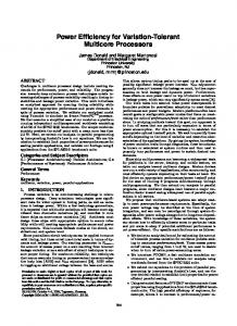
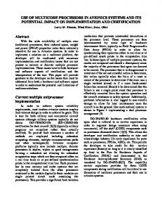
An intuitive measure of performance increase with pipeline depth is the change in CPI (Cycles Per Instruction) because adding more pipelines by using higher clock speeds and lower supply voltages generally lead to shorter logic depth, and therefore minimized delay. But the real measure of performance optimization with pipeline depth is to consider the MIPS (Million instructions per second)/BIPS (Billion instructions per second) or TPI (time per instruction) of the machine. TPI is the product of CPI and cycle time of the processor. As pipeline depth is increased, the cycle time goes down due to the fact that the entire logic time is fragmented into multiple numbers of intervals but the total time taken to process an instruction is not increased. Experimental results presented in [6], Figures 1,2 and 3, show the variation of CPI, cycle time and TPI, with pipeline depth respectively. It should be noted that these results are based on simulations on a particular machine [6] and there is a slight change in results when the micro-architecture is considered. Figure 4 shows that a theoretical estimate of the optimal pipeline depth could be 18/19.
Relative TPI
3.5 3 2.5 2 1.5 1
6
8
10
12
14 16 18 Number of pipeline stages
20
22
24
26
Fig. 3: Shows TPI as a function of pipeline depth
9 SPEC workloads Traditional workloads Modern workloads
8
Number of workloads
7 6 5 4 3 2 1
5
0 4.5
5−8
9−12
13−16 17−20 21−24 Pipeline depth
25−28
29−32
33−36
Fig. 4: Optimal pipeline depth for various benchmark applications
4
CPI
1−4
3.5
3
2.5
2
0
8
10
12
14 16 18 Pipeline stages
20
22
24
26
Fig. 1: Shows dependence of the CPI on the number of pipeline stages
It was found [6] that SPEC applications optimize a shorter pipeline depth than the traditional and modern workloads do. The difference between those workload models are depicted in Figure 4. These results are in accordance with the pipeline model of a four-issue superscalar out-of-order machine. If the degree of superscalarity is reduced, then the optimal pipeline depth will shift to the right, as shown in the theoretical derivation of optimal pipeline depth, given by: popt = (NI tp /αγNH t0 )1/2 ,
8
where NI is the instruction count, tp is the total logic delay, α -is the degree of superscalar processing, γ is the fraction of the total pipeline delay averaged overall hazards, NH is the hazard count, t0 is the cycle overhead, which itself depends on the technology. Some observations related to 1 are as follows:
7
Relative cycletime
(1)
6
5
4
•
The optimal pipeline depth increases for larger workloads with the large instruction count as well as for workloads with few hazards.
•
As the technology reduces the latch overhead (t0 ) and is relates to the total logic path (tp ), the optimum pipeline depth increases.
•
As the degree of the superscalar processing increases, the optimum pipeline depth decreases.
•
The optimal pipeline depth also increases with a decrease in fraction of hazards that causes a pipeline stall.
3
2
6
8
10
12
14 16 18 Number of pipeline stages
20
22
24
26
Fig. 2: Depicts the dependence of the cycle time on the pipeline depth
In the experimental analysis presented in [6], three different types of workloads were considered, namely, SPEC, Traditional, and Modern. The SPEC benchmark was written in C, the Traditional workloads were written in Assembly language and the Modern workloads were written in Java and C++.
III.
O UR C ONTRIBUTIONS
Several research works [11], [6] have been carried out dealing with optimal power and performance based on pipeline depth. Kunkel and Smith studied the pipeline depth and reported its impact on gate delays, particularly effect of performance on latch delays [12]. However, these works did not address certain optimal pipeline depths for all benchmarks and workloads. Due to this, we have studied dynamic pipeline stage unification. In this regards, minimizing the energy consumption to achieve a given task is a key concern for data centers that trend their smart phones, in the sense that: •
For feasibility purpose, temperature, power and battery capacities are limiting factors.
•
For cost saving purpose, lowering the energy enables smaller need for air-cooling, lower cost for ICs, packaging, space saving on PCB, etc.
•
For reliability purpose, lowering the temperatures might enable to remove mechanical devices, then reducing the risks of failure.
The dynamic voltage-frequency scaling (DVFS) is a well-known technique for reducing the power consumption, but its effectiveness decreases as the technology progresses. Currently, transistors made from a 45nm process are used. When the process technology hits 30nm and below, DVFS will not be of much use due to the fact that there will be a significant reduction in the threshold voltage level, which will cause a substantial increase in the current sub-threshold leakage. In order to work properly, the minimum supply voltage for transistors [13] must be 2.3Vth , where Vth is the threshold voltage. In addition, the supply level is very close to this value as transistors become smaller and the voltage scaling becomes difficult to realize. The DVFS technique degrades the reliability of a processor due to the increase of the transient fault probability. In future technologies, it is expected that transient faults will become a serious problem due to the lower supply voltages.
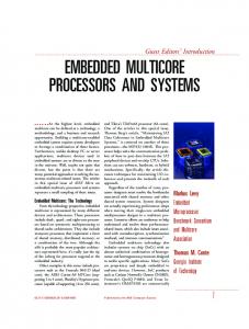
which indicates the sequence of programs to be executed. The second block is the decision module which decides whether VSP should be used or not and if so, then what extent of the VSP should be used. This decision module follows some prescribed rules while maintaining a task queue history with the corresponding VSP usage history. Based on these facts, the VSP conditions when programs are repeatedly executed are quickly determined. If this history data were absent, the decision module would have to compare every each program every time against some benchmark programs encoded in the decision module. In summary, the task queue history and the VSP usage history act like a look-aside buffers for the decision module saving time and energy. From the decision module, signals are sent to the VSP control module - which is a series of multiplexers that decide which steps of the pipeline will be by-passed. The control module is solely hardware-based. In Fig. 5, the arrow to VSP history could directly come from the decision unit itself instead of from the control unit.
Fig. 5: Proposed Approach
A. Functionality of Our Proposed System 1)
2)
To combat this limitation, this paper propose a different solution so-called variable stage pipelining (VSP). Our VSP technique dynamically scales the frequency in order to reduce the energy consumption as done in DVFS, but unlike DVFS, it unifies multiple pipeline stages by using the by-passing registers instead of scaling down the supply voltage, hence results in energy consumption saving in two different ways: 1)
VSP saves power consumption by reducing the total load capacitance of the clock driver. This is accomplished by stopping the clock signal to by-passed pipeline registers. VSP reduces the clock cycle count of the program execution by reducing the number of pipeline stages. As reported in [1], VSP is only moderately better than DVFS (45 nm). But as technology progresses, VSP is much better in terms of power-performance management compared to the DVFS technology.
2)
IV.
P ROPOSED A RCHITECTURAL F RAMEWORK
Our proposed approach for variable stage pipelining (VSP) is depicted in Fig. 5. The leftmost block is the task queue
3)
4)
First, we store the parameters of various benchmark programs/applications and related VSP configurations in the memory. These parameters include the instruction count, branch frequency, cache access frequency, number of integers, and floating point operations. For the first time, when a particular application is run by the user, VSP is not used. The parameters of the application are extracted from the processor and sent to the decision module. In this decision module, the parameters of the application that has just run are compared against those of the benchmark programs residing in memory, and a suitable VSP configuration is selected based on the nature of application program running on the processor and then stored in the VSP history. The application identifier and VSP configuration are stored against each other in a tabular form. This process is repeated for all applications for their first execution only, and a table of program identifiers vs. VSP configuration is built. In addition, a list of the most frequently used applications/programs with their VSP configurations is stored in the VSP history cache. We assume the infinite cache model is taken into consideration that as the pipeline depth increased, the latency also increases, but the access time remains constant. Therefore, there are no changes in optimum pipeline depth with regards to cache model [6]. For the execution of applications/programs, the decision module communicates with the task queue and fetches the identifier of the next program in queue.
Then, it tries to match the identifier with those present in the VSP history cache and when doing so, the VSP configuration is sent to the VSP control module which implements VSP in the processor. In case a cache is missed, the required match is brought into the cache and matched. This process is repeated again from Step 2. V.
VSP P ROPOSAL AND I MPLEMENTATION
This section presents the implementation of our approach and discusses its benefits in terms of energy savings. The basic idea behind VSP is to decrease the number of pipeline stages by by-passing a few stages. To achieve this, we use three signals: the clock/full-time clock, the part-time clock, and the unification signal. Clock/Full-time clock: The full-time clock signal is always active regardless of the unification. Part-time clock: The part-time clock signal is deactivated when the pipeline stages are unified. It is active when they are not unified. Unification signal: The unification signal indicates the pipeline stage unification. Since the pipeline register between two adjacent combinatorial logic circuits is inactive or by-passed, the two logic circuits operate together as a single stage.
where Tex is the execution time and Tex = NI /(IP C.f ) where NI is the instruction count, IPC is the number of instructions per cycle and f is the operating clock frequency. From Equations (2) and (3), the following equation involving the ratio of energy consumed when VSP is enabled and when the processor is at full power and speed, is obtained R(n) = IP Cf ull /IP Cvsp [1 − Pclock /Ptotal (1 − 1/n)], (4) where IP Cf ull is the number of instructions per cycle at full pipeline length and IP Cvsp is the IPC when VSP is in use. It should be noticed that IP Cf ull is less than IP Cvsp because of the shortened pipeline. Based on the above equation, the power and energy consumption are reduced in the inverse proportion of the IPC improvement. Also, the reduction depends on how much power is consumed by the clock driver with respect to the total power consumption of the processor. In modern processors, the ratio Pclock /Ptotal is considerably large, hence the power consumption can be greatly controlled. In [1], an example for 2-stage and 4-stage unification schemes is provided. A. Description of the VSP System •
The proposed VSP system uses software-hardware communication to decide whether to use VSP or not. If yes, it also has to decide what degree of unification is to be implemented. For this, the operating system has to look at the task scheduling queue and identify each application in the queue. Depending on the applications which are to be executed next, a message is sent to the control unit which activates or deactivates the VSP in the processor. For example, if the next immediate application is a game such as heavy programs (Table I), then to obtain a good performance, the processor must be run at full speed and full pipeline depth. Also, we cannot afford to use VSP as long as such heavy programs which is mentioned in Table I are running, even if other programs which are light or moderate are running in parallel. The decision factor for the use of VSP will be the presence or absence of heavy programs.
•
The limit on using VSP will always be decided by the heaviest program that is running or is scheduled to run immediately. This is due to the fact that an increase in the execution time nullifies the reduced power consumption profile. Also, it will lead to other undesirable effects such as application or operating system hanging. Therefore, if there are no heavy programs running or scheduled to run in the near future, the processor will make use of VSP to shorten the pipeline and save energy. Depending on the nature of the programs running, and which are scheduled to run immediately, the control unit which controls the VSP chooses the unification degree of either n = 1.25 or n = 1.5.
•
The control unit can be implemented using a simple method. One can use the unification method which uses simple logic to allow the multiplexer to select the registers which will be turned off i.e. by-passed. This method of implementation is useful when two different VSP schemes along with a normal full pipeline
The next question is how to by-pass a pipeline register? Several methods can be used to achieve this. Here, we propose two methods. In the first method, the pipeline register logic can be organized so that a signal can pass through it regardless of the clock signal when the VSP is enabled. This solution can be implemented if the pipeline registers are made up of transparent latches. This method is simple, but its only drawback is the cost-effectiveness of using transparent latches in the pipeline. In the second method, logic gates and multiplexors can be used. The multiplexors will decide which pipeline registers will be active and which ones will be shutdown when the unification signal is applied. An example of this solution is given in [14]. Now, let us understand how VSP lowers the energy consumption. VSP saves the power consumption by stopping the part-time clock. When a processor runs with a n-stage unification or unification-degree n, the power consumed by the clock drivers can be reduced by 1/n. In addition, as in the normal processors, the total power consumption is reduced by the clock frequency reduction rate. Thus, the power consumption of a VSP processor which runs at clock frequency fvsp with a unification degree n is expressed as follows: PV SP (fvsp , n) = (Ptotal − Pclock + Pclock /n).fvsp /fmax , (2) where PV SP is the power consumption when using VSP with an n-stage unification, Ptotal and Pclock are respectively the total power consumption of the processor and the power consumption of the clock drivers in the normal mode, fvsp is the frequency of the core when VSP is being used. The energy consumed EV SP is obtained as: EV SP (fvsp , n) = (Ptotal −Pclock +Pclock /n).fvsp /fmax .Tex (fvsp , n), (3)
scheme is used. Using (2), one can easily estimate how much power consumption is being saved. Ideally, if VSP is used for all the instructions, then one can save up to 60 percent power consumption, which is rarely the case; hence, assuming that VSP can be used only 60-70 percent of the time, we can save 30-40 percent of the power consumed at full pipeline depth and full clock frequency. B. Proposed Solution for Uni/Dual-core Processors We employ a processor and pipeline configuration similar to that introduced in [1] but with a different deeper pipeline having an extra ”nextPC” stage i.e. extra fetch and rename stage so that the maximum pipeline depth becomes 25 for LOAD operations and 23 for STORE, BRANCH and ALU operations when the VSP method is not in use. From [6], it was argued that the applications having different optimal pipeline depths were centred around 3 pipeline depth. For the different configurations and some applications, the number of pipeline stages was found to be round 16, 20 and 25. This forms the basis of our proposed solution. Starting with the proposed 23/25-staged pipeline, two different degrees of unification can be implemented, which are n=1.25 and n= 1.5. The case n=1.25 corresponds to a 20 stage and the case n= 1.5 corresponds to a 15 stage pipeline. Typically, CPU intensive applications (such as video, file compressing, gaming) need deeper pipelines for smooth running, hence while running these application, the use of VSP is not advisable since the run time of such programs may be significant, and thus may result in significant energy consumption [15] [16]. For moderately intense applications whose optimal pipeline length is around 20 stages, we use VSP with an approximate unification degree of n = 1.25 and for applications of low intensity, we use n = 1.5, thus bringing down the number of pipeline stages to 16. It should be noticed that fvsp is scaled the same way as the pipeline depth, hence, our proposed system has 3 pipeline configurations, namely, a 25-stage pipeline running at maximum clock frequency, a 20-stage pipeline running at 80% of the maximum clock frequency and a 16stage pipeline running at 67% of the maximum clock frequency [9]. Some commonly used applications are classified as heavy, moderate and light (as shown in Table I). Workloads and their characteristics, and related applications can be found in [10]. C. Proposed Solution for Multi-core Processors We have discussed the benefit of VSP as a technique to control power consumption in modern processors. In processors having 4 or more number of cores, VSP alone is not sufficient as technique for handling power management. We propose to complement VSP with the non-uniform clocking of different cores as follows. In one scheme, half the cores always run at full length pipeline, while the rest of the cores are available for pipeline length scaling. The cores which are not available for scaling are totally turned off when they are idle, i.e. those cores are only used for processing the instructions from heavy applications and when such applications are not running, these cores are said to be idle and are turned off, bringing down the power consumption of that core to less than 10% of its actual power consumption. In quad core processors, the remaining two cores available
for the VSP implementation are clocked uniformly either with VSP having unification degree of 1.25 or 1.5. In processors having higher number of cores such as 6, 8 and 12-core processors, there is a greater flexibility of implementing VSP as follows. One can make use of the cores which are available for VSP; or one can clock in a non-uniform way the cores which are available for VSP, by having special cores that will process only light intensity task instructions and cores that will process moderate intensity task instructions. If cores are idle, they are switched off. The switching of cores on and off can be done by using the method provided in [17]. Application
Type
Pipeline depth to be used
File compression
Heavy
Full-depth
Gaming
Heavy
Full-depth
Simulation software
Heavy
Full-depth
Video playback
moderate
VSP with n=1.25
Audio Playback
light
VSP with n = 1.5
Web Browser and related apps
light
VSP with n=1.5
Office programs
light
VSP with n=1.5
TABLE I: Load on Processor vs Pipeline depth
VI.
S IMULATION A NALYSIS
Our proposed approach needs to be automated from a use-case perspective getting the VSP to auto-tune and adapt to different software running on it for optimal performance. It is a lengthy implementation problem. Moreover, some of the parameters are still uncertain, and will vary during the implementation. For these reasons, we have taken the detailed cycle-accurate simulator M-SIM [18] and various embedded workloads of MiBench [19]. The I/O, memory and computationally intensive applications are simulated and obtained the execution time and power consumption of the various workloads. To define the processor parameters along with the pipeline depth, the following parameters are used in Equation (4); fvsp = fmax /degree of VSP and fmax =2.9 GHz (fmax is the maximum clock frequency of the processor). For various pipeline stages such as 16 (fvsp =1.94; Tex (fvsp,n )=532011.72), 20 (fvsp =2.32; Tex (fvsp,n )=442578.72) and 24 (fvsp =2.9; Tex (fvsp,n )=354062.97), R(n) is calculated using Equation (4) and the results are captured in Tables [II]-[IV]. n 1 1.25 1.5
PV SP (fvsp ,n) 240.7 235.1 231.3
EV SP (fvsp ,n)(in Billions) 128.06 125.08 123.09
R(n) 1.49 1.52 1.55
TABLE II: Number of Pipeline stages=16 vs. R(n)
n 1 1.25 1.5
PV SP (fvsp ,n) 287.4 280.7 276.2
EV SP (fvsp ,n)(in Billions) 127.20 124.24 122.26
R(n) 1.25 1.27 1.30
TABLE III: Number of Pipeline stages=20 vs. R(n)
n 1 1.25 1.5
PV SP (fvsp ,n) 359.2 350.9 345.3
EV SP (fvsp ,n)(in Billions) 127.20 124.24 122.26
R(n) 1.00 1.02 1.04
TABLE IV: Number of pipeline stages=24 vs. R(n)
2) EDP Results: In Figure 7, the results on EDP of various pipeline depth are presented. The pipeline depth 24 has the smallest EDP result compared to other pipeline depths such as 16 and 20. It is a deeper pipeline with a unification degree of n=1.25. Therefore, using 24-pipeline stage and a VSP unification degree of 1.25 design is the best configuration to achieve less EDP reduction in programs.
A. Tabulations of Pipeline Depth vs. Power/Performance Metrics
900 n=1 n=1.25 n=1.5
800
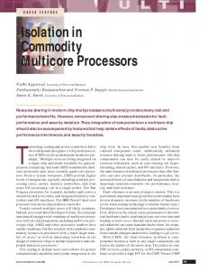
In this subsection, we study the relationship between the pipeline depth and power/performance metrics, for pipelines with various pipeline unification degrees. To study the efficiency of our proposed approach, the power and performance metrics [20] such as E, EDP and ED2 P are used. Using the following equations, the results obtained on power/performance metrics are summarized in Tables V-VII.
700
BIPS/W
600 500 400 300 200
E-Metric ⇐ BIPS/W ⇔ Instructions/W.s ⇔ Instructions/Energy
100 0 14
EDP ⇔ Energy (metric)∗Delay ⇔ (Energy/Instruction)∗Delay
16
ED2 P ⇔ Energy (metric)∗Delay2 ⇔ (Energy/Instruction)∗Delay2
n 1 1.25 1.5
16 809.24 828.52 842.13
20 677.75 693.92 705.23
18 20 22 Number of Pipeline Stages
24
26
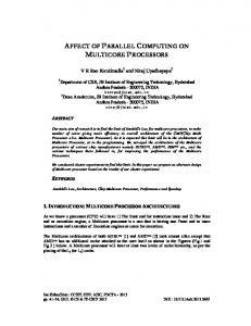
Fig. 6: Pipeline Depth vs. E-Metric
24 542.27 555.10 564.10
0.16 n=1 n=1.25
0.14
n=1.5 0.12
TABLE V: Pipeline Depth vs. E/Performance-only Metrics (BIPS/W) BIPS2/W
0.1
n 1 1.25 1.5
16 0.16 0.16 0.16
20 0.132 0.135 0.137
0.08
0.06
24 0.105 0.108 0.109
0.04
0.02
TABLE VI: Pipeline Depth vs. EDP Metrics (BIPS2 /W(in Billions))
0 14
16
18 20 22 Number of Pipeline Stages
24
26
Fig. 7: Pipeline Depth vs. EDP n 1 1.25 1.5
16 31000 31000 32000
20 25714 26328 26757
24 20574 21061 21403
4
3.5
TABLE VII: Pipeline Depth vs.
ED2 P
Metrics
(BIPS3 /W(in
x 10
n=1 n=1.25 n=1.5
Billions)) 3
1) Energy-only or Performance-only Metric: In Figure 6, the results on various pipeline depth with different unification degrees such as n=1, 1.25 and 1.5 are captured. It can be observed that shallow pipelines consume less energy than deeper pipelines. Therefore, if the E metric is used as the power/performance metric, one can apply shallow pipeline 16stage. It is also observed that a shallow pipeline with n=1.5 as VSP unification degree achieves the best efficiency. Since, the best performance relies on deeper pipelines, little performance achievements can be realized by applying the dynamic variable stage pipelining. Therefore, there is a limitation on implementing VSP when considering performance only platforms.
BIPS3/W
2.5
2
1.5
1
0.5
0 14
16
18 20 22 Number of Pipeline Stages
Fig. 8: Pipeline Depth vs. ED2 P
24
26
400 n=1 n=1.25 n=1.5
350
300 Power Consumption (W)
3) ED2 P Results: In this section, we study ED2 P results various pipeline depths and varied unification degrees. The results are captured in Figure 8. It can be observed that when using the ED2 P metric, the 16-stage design with unification degree of 1.5 achieves a better performance. If ED2 P reduction is considered for both power consumption and performance, the 24-stage pipeline design with unification degree of 1.25 attains yields the best results. This indicates that the dynamic pipeline stage unification is efficient in reducing the ED2 P processor.
250
200
150
100
50
VII.
D ISCUSSIONS
0 14
In this section, we study the relationship between pipeline depth and its efficiency along with pipeline stage unification, using M-SIM. In order to prove the efficiency of our proposed approach, the results are also verified through theoretical analysis. Tables II-IV summarizes the ratio of power and energy consumption (R(n)) while using variable stage pipelining. We have compared these results against the case where VSP is not enabled (i.e. when the unification degree n is equal to 1). From (4), we discussed on how our proposed technique effectively reduces the energy/power consumption rate by 1.5 to 2.5%. These results are also depicted in Figures 9-11. 1.6 n=1 n=1.25 n=1.5
1.4
1.2
R(n)
1
0.8
0.6
0.4
0.2
0 14
16
18 20 22 Number of Pipeline Stages
24
26
Fig. 9: Number of Pipeline stages vs. R(n)
140 n=1
n=1.25
n=1.5
16
18 20 22 Number of Pipeline Stages
24
26
Fig. 11: Power Consumption vs. R(n)
In Figure 9, the evaluation results of various number of pipeline stages with different unification degrees are depicted. The x-axis denotes the number of pipeline stages and the y-axis denotes the calculated R(n). The value of R(n) can be observed for the 3 stages separately. The values of R(n) for 16 pipeline stages increases when the value of n increases from 1 (VSP not enabled) to 1.25 and 1.5, indicating that when VSP is used, a better overall performance can be achieved in terms of power consumption. For 20 Pipeline Stages, the value of R(n) increases when the value of n increases increase, but not as drastically as in the case of the 16 pipeline stages. For 24 Pipeline Stages, the values of R(n) increases only very slightly when the the value of n increases. As can be observed in Figure 10, the pipeline stage unification has the following three unification degree: n = 1 - when VSP is not enabled, and n = 1.25 and 1.5. As we increase the unification value n from 1 to 1.25 and then 1.5, it can be observed that the power consumption decreases. This is also consistent with the theoretical expectation because when the value of n increases, more pipeline stages are unified, leading to less power consumption as can be seen from Table II. Consequently, the energy consumption also decreases as the value of n increases. In Figure 11, it can be observed that when the number of pipeline stages from 16, 20 and 24, the power consumption also increases. This is consistent with the theoretical expectation since deeper pipelines consume greater power.
Energy Consumption (joules/instruction)
120
100
80
60
40
20
0 14
16
18 20 22 Number of Pipeline Stages
24
Fig. 10: Energy Consumption vs. R(n)
26
According to the proposal on dynamic variable stage pipeline, an N stage pipeline (where N is the number of pipeline stages, for instance, 16, 20 and 24), can be dynamically change the unification degrees based on the application run on the processor. Paper [9] reported that the program may experience different phases of execution during the whole program. If the unification degree selects a suitable value, it can achieve better efficiency. This is also shown in Table I, where R(n) is consistent with the theoretical derivation because VSP is not beneficial for applications such as gaming and video compression which require deeper pipelines; rather, it is beneficial for less intensive applications in the sense that it can significantly improve their performance by unifying the stages in the pipeline, thereby reducing the power consumption.
VIII.
C ONCLUSION
We have proposed an automated dynamic pipeline-length controlling system and studied the relationship between pipeline depth and its efficiency when variable stage pipeline is used. Our results show that, if energy-only or performanceonly metric is considered, the 16-stage pipeline depth with unification degree of n=1.5 achieves a better result. By applying our variable stage pipelining method, we found that more EDP and ED2 P reduction can be achieved by deeper pipeline design. Among various pipeline depths, a 24- stage pipeline with unification degree of 1.25 can obtain smallest EDP. Similar conclusions were obtained for ED2 P when considering power and performance metrics. Our theoretical results also showed that for better efficiency purpose, the 16-stage pipeline design point with n=1.5 and the 24-stage with n=1.5 yield good results in terms of energy savings, especially when using the dynamic voltage frequency scaling (DVFS) and switching off selective core techniques. We believe that our proposed technique can be used for the design of novel multiprocessors which use transistors made of a sub 30nm process. As future work, we intend to develop new optimizing algorithms for the implementation of VSP based on workload classification and assessment.
[11]
[12]
[13] [14]
[15] [16]
[17]
[18]
[19]
[20]
R EFERENCES [1]
H. Shimada, H. Ando, and T. Shimada, “Pipeline stage unification: a low-energy consumption technique for future mobile processors,” in Proceedings of the 2003 international symposium on Low power electronics and design, ser. ISLPED ’03, 2003, pp. 326–329.
[2]
A. Jagannathan, H. H. Yang, K. Konigsfeld, D. Milliron, M. Mohan, M. Romesis, G. Reinman, and J. Cong, “Microarchitecture evaluation with floorplanning and interconnect pipelining,” in Proceedings of the 2005 Asia and South Pacific Design Automation Conference, ser. ASPDAC ’05, 2005, pp. 8–15.
[3]
M. S. Hrishikesh, K. I. Farkas, D. Burgert, S. W. Keckler, and P. Shivakumar, “The optimal logic depth per pipeline stage is 6 to 8 fo4 inverter delays,” in in Proceedings of the 29th Annual International Symposium on Computer Architecture, 2002, pp. 14–24.
[4]
D. Sager, D. P. Group, and I. Corp, “The microarchitecture of the pentium 4 processor,” Intel Technology Journal, vol. 1, 2001.
[5]
M. E. Thomadakis, “The architecture of the nehalem processor and nehalem-ep smp platforms,” 2011.
[6]
A. Hartstein and T. R. Puzak, “The optimum pipeline depth for a microprocessor,” SIGARCH Comput. Archit. News, vol. 30, no. 2, pp. 7–13, May 2002.
[7]
E. Sprangle and D. Carmean, “Increasing processor performance by implementing deeper pipelines,” in Proceedings of the 29th annual international symposium on Computer architecture, ser. ISCA ’02, 2002, pp. 25–34.
[8]
P. G. Emma and E. S. Davidson, “Characterization of branch and data dependencies on programs for evaluating pipeline performance,” IEEE Trans. Comput., vol. 36, no. 7, pp. 859–875, Jul. 1987.
[9]
J. Yao, H. Shimada, Y. Nakashima, S.-i. Mori, and S. Tomita, “Program phase detection based dynamic control mechanisms for pipeline stage unification adoption,” in Proceedings of the 6th international symposium on high-performance computing and 1st international conference on Advanced low power systems, ser. ISHPC’05/ALPS’06, 2008, pp. 494– 507.
[10]
A. M. G. Maynard, C. M. Donnelly, and B. R. Olszewski, “Contrasting characteristics and cache performance of technical and multi-user commercial workloads,” in Proceedings of the sixth international conference on Architectural support for programming languages and operating systems, ser. ASPLOS-VI, 1994, pp. 145–156.
V. Srinivasan, D. Brooks, M. Gschwind, P. Bose, V. Zyuban, P. N. Strenski, and P. G. Emma, “Optimizing pipelines for power and performance,” in Proceedings of the 35th annual ACM/IEEE international symposium on Microarchitecture, ser. MICRO 35, 2002, pp. 333–344. S. R. Kunkel and J. E. Smith, “Optimal pipelining in supercomputers,” SIGARCH Comput. Archit. News, vol. 14, pp. 404–411, May 1986. [Online]. Available: http://doi.acm.org/10.1145/17356.17403 “The itrs technology working groups. international technology roadmap for semiconductors (itrs),” http://public.itrs.net. J. Boucaron and A. Coadou, “Dynamic Variable Stage Pipeline: an Implementation of its Control,” http://hal.inria.fr/inria-00381563/PDF/RR6918.pdf, INRIA, Rapport de recherche RR-6918, 2009, rR-6918. M. J. Flynn, Computer Architecture: Pipelined and Parallel Processor Design, 1st ed. USA: Jones and Bartlett Publishers, Inc., 1995. J. L. Hennessy and D. A. Patterson, Computer Architecture, Fourth Edition: A Quantitative Approach. San Francisco, CA, USA: Morgan Kaufmann Publishers Inc., 2006. M. Ghasemazar, E. Pakbaznia, and M. Pedram, “Minimizing the power consumption of a chip multiprocessor under an average throughput constraint,” in ISQED, 2010, pp. 362–371. K. G. Joseph J. Sharkey, Dmitry Ponomarev, “Abstract M-SIM: A Flexible, Multithreaded Architectural Simulation Environment,” Tech. Rep., 2005. M. R. Guthaus, J. S. Ringenberg, D. Ernst, T. M. Austin, T. Mudge, and R. B. Brown, “Mibench: A free, commercially representative embedded benchmark suite,” in Proceedings of the Workload Characterization, 2001. WWC-4. 2001 IEEE International Workshop, ser. WWC ’01, 2001, pp. 3–14. R. Gonzalez and M. Horowitz, “Energy Dissipation In General Purpose Microprocessors,” IEEE Journal of Solid-State Circuits, pp. 1277–1284, (September) 1996.