PREDICTING EPHEMERAL GULLY LOCATION AND LENGTH USING TOPOGRAPHIC INDEX MODELS P. Daggupati, K. R. Douglas-Mankin, A. Y. Sheshukov
ABSTRACT. Ephemeral gullies (EGs) are incised channels resulting from concentrated overland flow that often form in a similar location every year. These erosional features add to producers’ management efforts and costs. Locating EGs and predicting their length is crucial for estimating sediment load and planning conservation strategies. Since topography plays an important role in the formation of EGs, this study investigated the prediction of EG location and length in two agricultural areas (S1 and S2) in two different physiographic regions using four topographic index models: compound topographic index (CTI), slope area (SA), wetness topographic index (WTI), and slope area power (SAP). The impacts of digital elevation model (DEM) resolution, agricultural land use mask data source, and topographic model critical thresholds were also evaluated. Automated geospatial models were developed to locate and derive EG length. Results show that the SA model predicted EG occurrence and length better than other models tested. The SA and CTI model predictions had similar patterns in terms of locating EG trajectory; however, the CTI model had greater discontinuity along the trajectory. The method developed to derive length in this study was sensitive to discontinuity, so the performance of the CTI model was poor. Finer-resolution DEMs (2 m) predicted EG location and lengths better than coarser-resolution DEMs (10 m or greater). Use of actual field-level reconnaissance data instead of NASS data for agricultural land use masking decreased false negative classification by 16% or more for all models. Detailed calibration of the SA model yielded different optimal thresholds for the two study regions: TSA = 30 for S1 and TSA = 50 for S2. Topographic index models were found to be useful in locating EGs and estimating expected lengths, but site-specific calibration of the topographic index model threshold was required, which might limit the general utility of these methods. Keywords. Ephemeral gully, Modeling, Sediment, Topography.
S
oil erosion by water in agricultural fields is a widespread land degradation problem (Montgomery, 2007) that occurs mainly through interrill and rill erosion, ephemeral gully (EG) erosion, and classical gully erosion. This study focuses on EG erosion, which is referred to as concentrated-flow erosion, mega-rill erosion, or shallow gully erosion. According to Foster (1986), EGs are larger than rills and smaller than classical gullies, and flow in EGs is clearly channelized. Definitions of EGs vary. According to the Soil Science Society of America (SSSA, 2008), EGs are “small channels eroded by concentrated overland flow that can be easily filled by normal tillage, only to reform again in the same location by additional runoff events.” Hauge (1977) and Poesen (1993) distinguished EGs from rills with a cross-
Submitted for review in December 2012 as manuscript number SW 10087; approved for publication by the Soil & Water Division of ASABE in July 2013. Contribution No. 13-189-J from the Kansas Agricultural Experiment Station, Manhattan, Kansas. The authors are Prasad Daggupati, ASABE Member, Postdoctoral Research Associate, Spatial Science Laboratory, Texas A&M University, College Station, Texas; Kyle R. Douglas-Mankin, ASABE Member, Professor, and Aleksey Y. Sheshukov, ASABE Member, Assistant Professor, Department of Biological and Agricultural Engineering, Kansas State University, Manhattan, Kansas. Corresponding author: Aleksey Sheshukov, 129 Seaton Hall, Kansas State University, Manhattan, KS 66506; phone: 785-532-5418; e-mail:
[email protected].
sectional area of 930 cm2 (1 ft2) or greater. According to Grissinger (1996a, 1996b), EGs are produced by concentrated flow erosion in swales or other topographically controlled locations and may be either a continuous or discontinuous extension of a drainage network. Smith (1993) defined EGs as small drainage channels that, if not filled in, would become permanent features of the drainage network. The importance of EG erosion is well established (Foster, 1986; Thorne et al., 1986; Poesen et al., 1996; Nachtergaele and Poesen, 1999; Poesen et al., 2003), but only a few process-based hydrologic or erosion models have included EG subroutines: Ephemeral Gully Erosion Model (EGEM; Woodward, 1999); Revised Ephemeral Gully Erosion Model (REGEM; Gordon et al., 2007); Chemicals, Runoff, and Erosion from Agricultural Management Systems (CREAMS; Knisel, 1980); Groundwater Loading Effects of Agricultural Management Systems (GLEAMS; Knisel, 1993); Water Erosion Prediction Project (WEPP; Flanagan and Nearing, 1995); and Annualized Agricultural Nonpoint Source Model (AnnAGNPS; Bingner and Theurer, 2003). These models, however, do not predict the location of EGs, which must be input into the models. A simple means of predicting the location of EG initiation is needed (Vandaele et al., 1996a; Vandekereckhove et al., 1998; Desmet and Govers, 1997; Knapen and Poesen, 2010). Souchere et al. (2003) reported that the development of models able to predict the location,
Transactions of the ASABE Vol. 56(4): 1427-1440
© 2013 American Society of Agricultural and Biological Engineers ISSN 2151-0032
1427
length, and cross-sectional area of EGs is of great importance. The concept of a topographic threshold is widely used to predict locations in the landscape where gullies may develop (Moore et al., 1988; Vandaele et al., 1996a; Vandekerckhove et al., 1998, 2000; Desmet et al., 1999; Knapen and Poesen, 2010; Poesen et al., 2011). The idea was first proposed by Horton (1945), who stated that a channel incision occurs when a threshold force is exceeded. Many studies used slope and drainage area to represent channel incision and found that an inverse relationship exists between drainage area and local slope that can be represented by a power-type equation (Patton and Schumm, 1975; Begin and Schumm, 1979; Vandaele et al., 1996a). Another concept that is widely used to identify the location of EGs is unit stream power. The EG formation depends on “generation of concentrated surface runoff of sufficient magnitude and duration to initiate and maintain erosion, leading to channelization” (Thorne and Zevenbergen, 1984). Concentrated surface runoff can be represented by specific stream power, which is a function of discharge, slope, and channel width. Drainage area multiplied by slope yields a parameter that can be used to represent total stream power (Desmet et al., 1999). The importance of topographic parameters such as slope and drainage area in locating EGs is well established. Another topographic parameter, plan curvature or convergence, also contributes to EG formation models because it provides the measure of the degree of flow convergence along the cross-section of a flow path (Zevenbergen and Thorne, 1987). Moore et al. (1991) indicated that slope (S), upstream drainage area (A), and plan curvature were primary topographic attributes that can be derived directly from digital elevation models (DEMs) and can be combined in some form (e.g., S⋅A or ln[A/S]) to characterize the spatial variability of specific processes occurring in the landscape; these combinations of primary topographic attributes are commonly referred to as topographic index models, topographic indices, secondary topographic attributes, compound attributes, or compound indices (Moore et al., 1991). In this study, the term “topographic index models” will be used to refer to models that represent combinations of primary topographic attributes. Several topographic index models were studied in the past few decades to predict the location of EGs. Thorne et al. (1986) used the CTI (compound topographic index) model to predict EG formation: tCTI = S⋅A⋅PLANC
(1)
where tCTI is a topographic EG index value, S is local slope (m m-1), A is upstream drainage area (m2), and PLANC is plan curvature (m per 100 m). Formation of an EG occurs when t exceeds some critical threshold value (T). Parker et al. (2007) tested the CTI model to predict EG locations in a GIS environment for different sites and found that TCTI varied from 5 to 62 depending on the study site, and that the general pattern of EGs predicted did not change when TCTI varied between 10 and 100.
1428
Moore et al. (1988) used two methods to estimate EG location: the SA (slope area index) model: tSA = S⋅As
(2)
and the WTI (wetness topographic index) model: tWTI = ln(As/S)
(3)
where tSA and tWTI are topographic EG index values, S is slope gradient (m m-1), and As is unit upstream drainage area (m2 m-1). Moore et al. (1988) found that EGs were constrained to areas for which S⋅As > 18 (i.e., TSA = 18) and ln(As/S) > 6.8 (i.e., TWTI = 6.8). Vandaele et al. (1996b) reported that the EG locations in a study area in south Portugal were better predicted using TSA = 40 and TWTI = 9.8. Vandaele et al. (1996a) used the SAP (slope area power index) model: tSAP = S⋅Asb
(4)
where tSAP is a topographic EG index value, S is slope gradient (m m-1), As is unit contributing area (m2 m-1), and b is an empirical coefficient commonly assumed to be 0.4 (Vandaele et al., 1996a, 1996b; Desmet et al., 1999). Vandaele et al. (1996a) tested the model in the Kinderveld catchment in Spain and found out that TSAP = 0.486 was needed for locating initiation points of EGs. In separate studies, Desmet et al. (1999) reported that TSAP = 0.75 and Vandaele et al. (1996b) reported that TSAP = 1.0 performed better in predicting location of EGs in their study areas. The topographic index models discussed above were used to locate the EGs. Although the importance of length is well established, none of these studies used these topographic index model results to derive EG length (Woodward, 1999; Nachtergaele et al., 2001a, 2001b; Capra et al., 2005, 2009; Gordon et al., 2007; Poesen et al., 2011). Length of an EG is an important parameter because it is needed as an input by process-based models, such as EGEM and WEPP, to estimate EG sediment losses (Woodward, 1999). Nachtergaele et al. (2001a, 2001b) reported a strong correlation between EG length and volume of soil eroded. Length of an EG also can be used to estimate EG volume using simple models (Capra et al., 2005, 2009; Poesen et al., 2011). Gordon et al. (2007) reported that topographic index models are used to locate potential EG locations, but no method is currently available to predict EG length. The goal of this study was to evaluate existing topographic index models (CTI, SA, WTI, and SAP) in predicting EG location and length within agricultural fields according to two metrics: occurrence (presence or absence within a given area) and length (total accumulated length within a given area). Specific objectives were to (1) develop a GIS-based methodology to locate and derive length of EGs using existing topographic index models, (2) compare and evaluate the impacts of DEM resolution (2 m, 10 m, and 30 m) and agricultural land use mask data source (NASS or field reconnaissance) on EG occurrence and length predictions, and (3) evaluate the impacts of topographic index model thresholds (T) on EG occurrence and length predictions.
TRANSACTIONS OF THE ASABE
STUDY AREA Two study areas where EGs are a major concern were selected. Study area 1 (S1) is located in Douglas County in northeastern Kansas, and study area 2 (S2) is located in Reno County in south central Kansas (fig. 1). S1 has an area of 4,359 ha (10,771 ac) (43% cropland), and S2 encompasses 1,927 ha (4,762 ac) (81% cropland). Grain sorghum and corn were the major crops in S1, and wheat was the major crop in S2. The EGs in S1 were smaller (mostly single EGs; average length: 210 m) and narrower, whereas the EGs in S2 were larger (mostly branched EGs; average length: 408 m) and wider. The average catchment in which EGs were present was 2.5 ha (6.2 ac) with 1.7% slope in S1 and 2.35 ha (5.8 ac) with 0.97% slope in S2. In this study, S1 was used for evaluating performance of all topographic models, whereas S2 was used for verification of the best model.
METHODS DIGITIZING EGS IN STUDY AREAS One or more EGs were seen in many agricultural fields across the study areas during field reconnaissance surveys in 2009, 2010, and 2011, especially after rain events
(Daggupati et al., 2010); however, field measurements of EG characteristics (e.g., length, width, and depth) were not possible because access to the agricultural fields (private land) in both study watersheds was limited. Because of this limitation, we drove on public roads in the study areas and recorded the fields that were observed to have EGs. During field reconnaissance, a common landuse unit (CLU) field boundary shapefile was edited in ArcGIS on a laptop computer to record fields with EGs. In the lab, the shapefile of fields with EGs was overlaid on a corresponding aerial image. The 2010 National Agricultural Imagery Program aerial image was selected for S1, and the 2003 Digital Ortho Quarter Quadrangle aerial image was selected for S2 because EGs could be clearly identified on these images. Aerial images from other years (1995 through 2011) were also acquired, but locating EGs was difficult on these images since they were taken during the crop growing season when a crop canopy was fully established. EGs were manually digitized over the aerial images in the study areas in the fields where EGs were observed during field visits. Extreme care was taken to digitize the trajectory of each EG located on the aerial image. Starting and ending points of each EG were difficult to determine precisely. Color changes on an aerial image and our expert judgment were used to digitize accurately,
S1
S2
Figure 1. Study areas S1 and S2 showing digitized ephemeral gullies.
56(4): 1427-1440
1429
Model CTI SA WTI SAP
Table 1. EG topographic index models and thresholds tested in S1. Equation Eq. No. Thresholds (T) References (1) 12, 62, and 100 Thorne et al. (1986), Parker et al. (2007) tCTI = S⋅A⋅PLANC (2) 5, 18, and 40 Moore et al. (1988), Vandaele et al. (1996a) tSA = S⋅As (3) 6.8, 9.8, and 12 Moore et al. (1988), Vandaele et al. (1996b) tWTI = ln(As/S) (4) 0.3, 0.5, and 1 Vandaele et al. (1996a, 1996b), Desmet et al. (1999) tSAP = S⋅As0.4
with an estimated error of approximately 5% of EG length. Google Earth together with hill-shade images (which enhanced the relief of the surface) were used to verify and cross-check the location during the digitizing process. Many EGs (69% in S1, 38% in S2) were seen on the aerial image within the study area but were not visible from the windshield during the field visit for several reasons: (1) EGs were located far away from roads or obscured by topographic features, (2) established crops concealed the EGs during the field visit, or (3) multiple EGs were located within one field. EGs that were located on the aerial image but were not seen during the field visit were also digitized. Because this study compared model-simulated EGs to observed EGs (i.e., digitized EGs on the aerial image), including all EGs was considered essential. Finally, the digitized EGs were used as observed or reference data to evaluate performance of the topographic index models. EG TOPOGRAPHIC INDEX MODELS AND THRESHOLDS Four published EG topographic index models were used to predict EG location (table 1). EG topographic index models determine the presence or absence of an EG at each point (i.e., in a pixel) within a given area for which the topographic EG index value (t in eqs. 1 through 4) exceeds a threshold value (T). For the CTI and SAP models, the three (minimum, middle, and maximum) values of T were selected based on values reported in the literature (12, 62, and 100 for the CTI model, and 0.3, 0.5, and 1 for the SAP model). For the SA model, the new value of 5 was added to widen the default reported range of 18 to 40 to seek better identification of EGs, whereas for the WTI model the maximum value was increased to 12 from the default range of 6.8 to 9.8 because no ephemeral gullies were recorded within that range. DATA INPUTS FOR TOPOGRAPHIC INDEX MODELS DEMs provide key data for topographic index models. Topographic attributes, such as slope, upstream drainage area, and plan curvature are directly derived from DEMs. Many studies have investigated the impact of DEM resolution for evaluating model responses to changes in topographic attributes and have concluded that DEM resolution substantially affects topographic attributes and thereby model results (Holmes et al., 2000; Chaubey et al., 2005; Parker et al., 2007; Momm et al., 2011). Impacts of DEM resolution (2 m, 10 m, and 30 m) on the performance of topographic index models were evaluated in S1 to correctly predict EG location. EGs within agricultural fields were of interest in this study; therefore, land use was used as an input to mask areas other than agricultural fields. Daggupati et al. (2011) reported that the land use data source has a major impact on modeling results for field-scale targeting, so this study
1430
evaluated the impacts on topographic index model performance of masking agricultural lands using either USDA National Agricultural Statistical Service (NASS) data or field reconnaissance land use data. Field reconnaissance land use data were collected during EG field reconnaissance in 2011, described above. Field boundaries used for both data sources were digitized manually using high-resolution aerial images. Care was taken to exclude waterways from the digitized land use. METHODOLOGY TO LOCATE EGS An automated geospatial model was built in a GIS environment (ESRI, 2011) using a model builder platform (Daggupati, 2012) to locate EGs for each of the topographic index models. The geospatial model requires elevation (DEM), land use, and roads as inputs. When the inputs are satisfied, the model calculates topographic attributes such as local slope, upstream drainage area, unit upstream drainage area, and plan curvature from the DEM. Filling a DEM or removing pits was not recommended by Kim (2007) and Bussen (2009) in gully-related studies because doing so fills out natural depressions that are important to EG formation; therefore, pit removal was not applied in this study. After the required topographic attributes are generated, the geospatial model calculates the topographic index value (t) for each pixel in the study area and compares that value to the user-defined threshold (T) for the topographic index model being used. If the pixel value of t is greater than T, then an EG pixel is located on the output raster (fig. 2). Because our interest was in identifying EGs only in agricultural fields, the geospatial model used land use and roads to mask non-agricultural areas. METHODOLOGY TO ESTIMATE EG LENGTH Several post-processing techniques were developed to derive length of EGs from the output raster (generated for each topographic index model from the geospatial model discussed above) using the following steps: • Pixels that represent EGs in the output raster of a topographic index model were converted into a polyline shapefile (fig. 3a). • The polylines within the trajectory of an EG were sometimes disconnected (fig. 3a) (i.e., some points along an apparent EG trajectory did not meet the given threshold). To make the polylines continuous within the trajectory of an EG, the polylines were “snapped” to each other using a snapping rule of 5 m (i.e., two lines that were 5 m apart, or less, were joined) (fig. 3b). Higher snapping distance (>5 m) resulted in lines snapping to other lines that were not part of the EG trajectory, thus distorting the shape along the trajectory (most prevalent in branched
TRANSACTIONS OF THE ASABE
used. All individual polylines within a catchment were dissolved to a single polyline, which was considered an EG with a unique identification number. • EGs shorter than 50 m were removed. Using the above steps, EGs were given a length and a unique identification number so that they could be used either as input to the process-based model or to estimate soil loss volume using empirical relationships. It should be noted that lengths obtained by this method are “potential lengths” derived from topographic attributes and do not consider any processes occurring during the formation of EGs. It should also be noted that some discontinuity within lengths may remain along an EG trajectory. An automated geospatial model was developed in the ArcGIS environment using the model builder platform to automate the process of deriving lengths of EGs and eliminate the tedious steps outlined above.
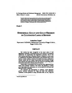
Figure 2. Ephemeral gully (EG) pixels in an agricultural field in study area 1 (S1).
EGs); consequently, snapping distance greater than 5 m was not used in this study. • The lengths of the polylines were calculated, and lengths smaller than 10 m were removed (fig. 3c). • At this point, each polyline had its own identification number, and many EGs were represented by multiple polylines. Catchments were developed separately using the DEM (areas outlined by blue lines in fig. 3d), and each individual polyline within a catchment was given a unique identification number (fig. 3d). The size of the catchment is user-defined and can be varied. In this study, 1 ha catchments were
PERFORMANCE OF TOPOGRAPHIC INDEX MODELS There is no established method to compare and evaluate the performance of topographic index models. Desmet et al. (1999) compared the percentage of predicted EG pixels that corresponded to the location of observed EG pixels. Parker et al. (2007) used visual interpretation by comparing potential EG pixels generated by the model to observed EG pixels. Performance of each topographic index model to predict EG location and length was assessed by three methods: (1) visual evaluation of EG trajectories, (2) error matrix assessment of model performance in correctly identifying EG occurrence (presence or absence) within a given area, and (3) statistical assessment of model performance in correctly identifying EG length (total accumulated length) within a given area.
Visual Evaluation Locations of EGs (model predictions along the trajectory) and derived lengths were evaluated using visual comparison of digitized EGs to model-simulated EG
Figure 3. Steps in deriving the length of ephemeral gullies (EGs): (a) EG raster converted to polyline, (b) polylines snapped, (c) length of EGs calculated and smaller lengths (