Prediction in Projection Joshua Garland1, a) and Elizabeth Bradley2, b) 1)
University of Colorado Department of Computer Science Boulder, Colorado 80303, USA 2) University of Colorado Department of Computer Science, Boulder, Colorado 80303, USA and the Santa Fe Insitute, Santa Fe, New Mexico (Dated:; Revised)
arXiv:1503.01678v1 [nlin.CD] 5 Mar 2015
ABSTRACT
Prediction models that capture and use the structure of state-space dynamics can be very effective. In practice, however, one rarely has access to full information about that structure, and accurate reconstruction of the dynamics from scalar time-series data—e.g., via delaycoordinate embedding—can be a real challenge. In this paper, we show that forecast models that employ incomplete embeddings of the dynamics can produce surprisingly accurate predictions of the state of a dynamical system. In particular, we demonstrate the effectiveness of a simple near-neighbor forecast technique that works with a two-dimensional embedding. Even though correctness of the topology is not guaranteed for incomplete reconstructions like this, the dynamical structure that they capture allows for accurate predictions—in many cases, even more accurate than predictions generated using a full embedding. This could be very useful in the context of real-time forecasting, where the human effort required to produce a correct delay-coordinate embedding is prohibitive.
on fast time scales. In this paper, we show that the full effort of delay-coordinate embedding is not always necessary when one is building forecast models, and can indeed be overkill. Using synthetic time-series data generated from the Lorenz-96 atmospheric model and real data from a computer performance experiment, we demonstrate that a two-dimensional embedding of scalar timeseries data from a dynamical system gives simple forecast methods enough traction to generate accurate predictions of the future course of those dynamics—sometimes even more accurate than predictions created using the full embedding. Since incomplete embeddings do not preserve the topology of the full dynamics, this is interesting from a mathematical standpoint. It is also potentially useful in practice. This reduced-order forecasting strategy involves only one free parameter (τ ), good values for which, we believe, can be estimated ‘on the fly’ using information-theoretic and/or machine-learning algorithms. As such, it sidesteps much of the complexity of the embedding process—perhaps most importantly, the need for expert human interpretation—and thus could enable automated, real-time dynamics-based forecasting in practical applications.
LEAD PARAGRAPH I.
Prediction models constructed from state-space dynamics have a long and rich history, dating back to roulette and beyond. A major stumbling block in the application of these models in real-world situations is the need to reconstruct the dynamics from scalar time-series data—e.g., via delay-coordinate embedding. This procedure, which is the topic of a large and active body of literature, involves estimation of two free parameters: the dimension m of the reconstruction space and the delay, τ , between the observations that make up the coordinates in that space. Estimating good values for these parameters is not trivial; it requires the proper mathematics, attention to the data requirements, computational effort, and expert interpretation of the results of the calculations. This is a major challenge if one is interested in real-time forecasting, especially when the systems involved operate
a) Electronic b) Electronic
mail:
[email protected] mail:
[email protected]
INTRODUCTION
Complicated nonlinear dynamics are ubiquitous in natural and engineered systems. Methods that capture and use the state-space structure of a dynamical system are a proven strategy for forecasting the behavior of systems like this, but the task is not straightforward. The governing equations and the state variables are rarely known; rather, one has a single (or perhaps a few) series of scalar measurements that can be observed from the system. It can be a challenge to model the full dynamics from data like this, especially in the case of forecast models, which are only really useful if they can be constructed and applied on faster time scales than those of the target system. While the traditional state-space reconstruction machinery is a good way to accomplish the task of modeling the dynamics, it is problematic in real-time forecasting because it generally requires input from and interpretation by a human expert in order to work properly. The strategy suggested in this paper sidesteps that roadblock by using a reduced-order variant of delay-coordinate embedding to build forecast models for nonlinear dynamical
2 systems. Modern approaches to modeling a time series for the purposes of forecasting arguably began with Yule’s work on predicting the annual number of sunspots1 through what is now known as autoregression. Before this, timeseries forecasting was done mostly through simple global extrapolation2 . Global linear methods, of course, are rarely adequate when one is working with nonlinear dynamical systems; rather, one needs to model the details of the state-space dynamics in order to make accurate predictions. The usual first step in this process is to reconstruct that dynamical structure from the observed data. The state-space reconstruction techniques proposed by Packard et al.3 in 1980 were a critical breakthrough in this regard. In the most common variant of this now-classic approach, one constructs a set of vectors ~xj ∈ Rm where each coordinate is simply a timedelayed element of the scalar time-series data xj , i.e., ~xj = [xj xj−τ . . . xj−(m−1)τ ] for τ > 0. In 1981, Takens showed that this delay-coordinate embedding method provides a topologically correct representation of a nonlinear dynamical system if a specific set of theoretical assumptions are satisfied4 ; in 1991, Sauer et al. extended this discussion and relaxed some of the theoretical restrictions5 . This remains a highly active field of research; see, for example, Abarbanel6 or Kantz & Schreiber7 for surveys. A large number of creative strategies have been developed for using the state-space structure of a dynamical system to generate predictions (e.g.,2,8–12 ). Perhaps the most simple of these is the “Lorenz Method of Analogues” (LMA), which is essentially nearest-neighbor prediction13 . Lorenz’s original formulation of this idea used the full system state space; this method was extended to embedded dynamics by Pikovsky12 , but is also related to the prediction work of Sugihara & May11 , among others. Even this simple strategy—which, as described in more detail in Section II B, builds predictions by looking for the nearest neighbor of a given point and taking that neighbor’s observed path as the forecast—works quite well for forecasting nonlinear dynamical systems. LMA and similar methods have been used successfully to forecast measles and chickenpox outbreaks11 , marine phytoplankton populations11 , performance dynamics of a running computer14–16 , the fluctuations in a far-infrared laser2,10 , and many more. The reconstruction step that is necessary before these methods can be applied to scalar time-series data, however, can be problematic. Delay-coordinate embedding is a powerful piece of machinery, but estimating values for its two free parameters, the time delay τ and the dimension m, is not trivial. A large number of heuristics have been proposed for this task (e.g.,7,17–28 ), but these methods, described in more detail in Section II A, are computationally intensive and they require input from— and interpretation by—a human expert. This can be a real problem in a prediction context: a millisecond-scale forecast is not useful if it takes seconds or minutes to
produce. And it is even more of a problem in nonstationary systems, since the reconstruction machinery is only guaranteed to work for an infinitely long noise-free observation of a single dynamical system. If effective forecast models are to be constructed and applied in a manner that outpaces the dynamics of the target system, then, one may not be able to use the full, traditional delaycoordinate embedding machinery to reconstruct the dynamics. The goal of the work described in this paper was to sidestep that problem by developing prediction strategies that work in incomplete embedding spaces. The conjecture that forms the basis for our work is that a full formal embedding, although mandatory for detailed dynamical analysis, is not necessary for the purposes of prediction. As a first step towards validating that conjecture, we constructed two-embeddings from a number of different time-series data sets, both simulated and experimental, and then built forecast models in that space. Sections III and IV of this paper present and discuss those results in some detail. In short, we found that forecasts produced using the Lorenz method of analogues on a two-dimensional delay-coordinate embedding are roughly as accurate as—and often even more accurate than— forecasts produced by the same method working in the full embedding space. Figure 1 shows a quick example: a pair of forecasts of the so-called “Dataset A”, a time series from a far-infrared laser from the Santa Fe Institute prediction competition2 , generated with LMA on full and 2D embeddings. The main point of Figure 1—and the main claim of this paper—concerns the similarity of the two panels. The forecast generated in the full embedding space is not much more accurate than the one generated in the two-dimensional reconstruction. The errors between true and predicted values were 0.117 and 0.148, respectively, as measured using the assessment procedure and error metric covered in Section II B; a better choice of τ , as described in Section IV, brings the latter value down to 0.119. That is, even though the low-dimensional reconstruction is not completely faithful to the underlying dynamics, it appears to be good enough to support accurate forecast models of nonlinear dynamics. Both of these LMA-based forecasts, incidentally, significantly outperformed traditional strategies like random-walk (by a factor of ≈ 8.5) and autoregressive integrated moving average (by a factor of ≈ 6.5). The results in Sections III and IV offer a deeper validation of the claim that the full complexity (and effort) of the delay-coordinate ‘unfolding’ process may not be strictly necessary to the success of forecast models of real-world nonlinear dynamical systems. In effect, the reduced-order modeling strategy that we propose is a kind of balance of a tradeoff between the power of the state-space reconstruction machinery and the effort required to use it. Fixing m = 2 effectively avoids all of the in-depth, post-facto, data-dependent analysis that is required to properly estimate a value for this parameter—
300
300
250
250
200
200
pj and cj
pj and cj
3
150 100
150 100 50
50
0
0 1100 1200 1300 1400 1500 1600 1700 1800 1900
time (j) (a) LMA in the full embedding space (“fnn-LMA”)
1100 1200 1300 1400 1500 1600 1700 1800 1900
time (j) (b) LMA in a two-dimensional embedding space (“ro-LMA”)
FIG. 1: Forecasts of SFI data set A using Lorenz’s method of analogues in (a) full and (b) 2D reconstructions of the state-space dynamics. Blue os are the true continuation cj of the time series and red xs (pj ) are the forecasts; black error bars are provided if there is a discrepancy between the two. Embedding parameter values were estimated using standard techniques: the first minimum of the average mutual information23 for the delay in both images and the false near neighbor method of Kennel et al.25 , with a threshold of 20%, for the dimension in the left-hand image. Even though the 2D embedding used in (b) is not faithful to the underlying topology, it enables successful forecasting of the time series.
which is arguably the harder part of the process. It also avoids the high computational complexity that is involved in near-neighbor searches in high-dimension state spaces—an essential step in almost any forecast strategy. Of course, there is still a free parameter: the delay τ . As described in Section IV, though, we believe that good values for this parameter can be estimated ‘on the fly,’ with little to no human guidance, which would make this method both agile and resilient. No forecast model will be ideal for every task. In fact, as a corollary of the undecidability of the halting problem29 , no single forecasting schema is ideal for all noise-free deterministic signals2 —let alone all real-world time-series data sets. We do not want to give the impression that the strategy proposed here will be effective for every time series, but we do intend to show that it is effective for a broad spectrum of signals. Additionally, we want to emphasize that it is a short-term forecasting scheme. Dimensional reduction is a double-edged sword; it enables on-the-fly forecasting by eliminating a difficult estimation step, but it effects a guaranteed information loss in the model. This well-known effect2 all but guarantees problems with accuracy as prediction horizons are increased. We explore this limitation in Section III A.
II.
BACKGROUND AND METHODS
A.
Delay-Coordinate Embedding
The process of collecting a time series {xj }N j=1 from a dynamical system (aka a “trace”) is formally the evaluation of an observation function h : X → R at the true system state ~y (tj ) at time tj for j = 1, .., N , i.e., xj = h(~y (tj )) for j = 1, . . . , N 5 . Provided that the un-
derlying dynamics Φ and the observation function are both smooth and generic, Takens4 proves that the delay coordinate map: F (h, Φ, τ, m)(~y (tj )) = ([xj xj−τ . . . xj−(m−1)τ ]T ) (1) from a d-dimensional smooth compact manifold M to R2d+1 is a diffeomorphism on M . To assure topological conjugacy, the proof requires that the embedding dimension m must be at least twice the dimension d of the ambient space; a tighter bound of m > 2dcap , the capacity dimension of the original dynamics, was later established by Sauer et al.5 . Operationalizing either of these theoretical constraints can be a real challenge. d is not known and accurate dcap calculations are not easy with experimental data. The theoretical constraints on the time delay are less stringent: τ must be greater than zero and not a multiple of any orbit’s period4,5 . In practice, however, the noisy and finite-precision nature of digital data and floating-point arithmetic combine to make the choice of τ much more delicate7 . As mentioned in the previous section, the forecast strategy proposed in this paper sidesteps the challenge of estimating the embedding dimension by fixing m = 2. Selection of a value for the remaining free parameter, τ , is still an issue, though. There are dozens of methods for this—e.g.,7,17–23 . In this paper, we use the method of mutual information 22,23 , in which τ is chosen at the first minimum of the time-delayed mutual information, calculated using the TISEAN package28 . Fraser & Swinney argue that this minimizes the redundancy of the embedding coordinates, thereby maximizing the information content of the overall delay vector23 . This choice is discussed and empirically verified by Liebert and Schuster22 , although agreement on this topic is by no means universal30,31 . And it is well known that choice of τ is application-
4 and system-specific: a τ that works well for a Lyapunov exponent calculation may not work well for other purposes7,20,32 . Indeed, as we show in Section IV, the τ value suggested by mutual information calculations is rarely the optimal choice for our reduced-order forecast strategy. Even so, it is a reasonable starting point, as it is the standard technique used in the dynamical systems community. The embedding dimension m is not a parameter in our reduced-order forecasting strategy. Since full embeddings are the point of departure for the central premise of this paper, however—and the point of comparison for our results—we briefly review methods used to estimate values for that parameter. As in the case of τ , a number of creative strategies for doing so have been developed over the past few decades7,19,21,25–28 . Most of these are based in some way on minimizing the number of false crossings that are caused by projection. In this paper, we use the false near neighbor (FNN) approach of Kennel et al.25 , calculated using TISEAN28 with a ≈ 20% threshold on the percentage of neighbors. (Whenever we refer to a “full” embedding, as in the discussion of Figure 1, we mean that the m value was estimated in this fashion and the τ value was chosen at the first minimum of the mutual information, as described in the previous paragraph.) Again, no heuristic method is perfect, but FNN is arguably the most widely used method for estimating m, and thus is useful for the purposes of comparison. Finally, it should be noted that there is an alternative view that one should estimate τ and m together, not separately20,24,27,33 .
B.
Lorenz Method of Analogues
As mentioned in Section I, the dynamical systems community has developed a number of methods that capture and use state-space structure to create forecasts. Since the goal of this paper is to offer a proof of concept of the notion that incomplete embeddings could give these kinds of methods enough traction to generate useful predictions, we chose one of the oldest and simplest members of that family: Lorenz’s method of analogues (LMA). In future work, we will explore reduced-order versions of other forecast strategies. To apply LMA to a scalar time-series data set {xj }nj=1 , one begins by performing a delay-coordinate embedding using one or more of the heuristics presented in Section II A to choose m and τ . This produces a trajectory of the form: {~xj = [xj xj−τ . . . xj−(m−1)τ ]T }nj=1−(m−1)τ Forecasting the next point in the time series, xn+1 , amounts to reconstructing the next delay vector ~xn+1 in the trajectory. Note that, by the form of delay-coordinate vectors, all but the first coordinate of ~xn+1 are known. To choose the first coordinate, one finds the nearest neighbor
of ~xn in the reconstructed space—namely ~xj(1,m) —and maps that vector forward using the delay map, obtaining ~xj(1,m)+1 = [xj(1,m)+1 xj(1,m)+1−τ . . . xj(1,m)+1−(m−1)τ ]T Using the neighbor’s image, one defines p~n+1 = [xj(1,m)+1 xn+1−τ . . . xn+1−(m−1)τ ]T LMA defines the forecast of xn+1 as pn+1 = xj(1,m)+1 . If performing multi-step forecasts, one appends the new delay vector p~n+1 = [xj(1,m)+1 xn+1−τ . . . xn+1−(m−1)τ ]T to the end of the trajectory and repeats this process as needed. Many more-complicated variants of this algorithm have appeared in the literature (e.g.,2,8,9,11 ), most of which involve building some flavor of local-linear models around each delay vector and then using it to make the prediction of the next point. Here, we use the basic version, in two ways: first—as a baseline for comparison purposes—on a “full” embedding of each time series, with m chosen using the false near neighbor method of Kennel et al.25 on that data; second, with m = 2. In the rest of this paper, we will refer to these as fnn-LMA and ro-LMA, respectively. The experiments reported in Section III use the same τ value for both fnn-LMA and ro-LMA, choosing it at the first minimum of the time-delayed mutual information of the time series23 . In Section IV, we explore the effects of varying τ on the accuracy of both methods. C.
Assessing Forecast Accuracy
To evaluate ro-LMA and compare it to fnn-LMA, we calculate a figure of merit in the following way. We split each N -point time series into two pieces: the first 90%, referred to as the “initial training” signal and denoted {xj }nj=1 , and the last 10%, known as the “test” signal (k+n+1)=N
{cj }j=n+1 . We use the initial training signal to build the model, following the procedures described in the previous section. We use that model to generate a prediction pn+1 of the value of xn+1 , then compare pn+1 to the true continuation, cn+1 . The initial investigations that are reported in Section III involve “one-step” models, which are rebuilt after each step, out to the end of the test signal, using {cn+1 } ∪ {xj }nj=1 . In Section IV, we extend this conversation to longer prediction horizons. As a numerical measure of prediction accuracy, we calculate the mean absolute scaled error (M ASE)34 between the true and predicted signals: M ASE =
k+n+1 X k j=n+1 n−1
|pj − cj | Pn i=2 |xi − xi−1 |
M ASE is a normalized measure: the scaling term in the denominator is the average in-sample forecast error for a
5 random-walk prediction—which uses the previous value in the observed signal as the forecast—calculated over the initial training signal {xj }nj=1 . That is, M ASE < 1 means that the prediction error in question was, on the average, smaller than the in-sample error of a randomwalk forecast on the same data. Analogously, M ASE > 1 means that the corresponding prediction method did worse, on average, than the random-walk method. The M ASE value of 0.117 for Figure 1, for instance, means 1 that the fnn-LMA forecast of the SFI data set A was 0.117 times better than a random-walk forecast of the initial training portion of same signal. While its comparative nature may seem odd, this error metric allows for fair comparison across varying methods, prediction horizons, and signal scales, making it a standard error measure in the forecasting literature—and a good choice for the study described in the following sections, which involve a number of very different signals. III.
PREDICTION IN PROJECTION
In this section, we demonstrate that the accuracies of forecasts produced by ro-LMA—Lorenz’s method of analogues, operating on a two-dimensional embedding of a trajectory from a dynamical system—are similar to and often better than forecasts produced by fnn-LMA, which operates on a full reconstruction of the same dynamics. While the brief example in Section I is a useful first validation of that statement, it does not support the kind of exploration that is necessary to properly evaluate a new forecast method, especially one that violates the basic tenets of delay-coordinate embedding. The SFI data set A is a single trace from a single system. We want to show that ro-LMA is comparable to or better than fnn-LMA for a range of systems and parameter values—and to repeat each experiment for a number of different trajectories from each system. To this end, we studied two dynamical systems, one simulated and one real: the Lorenz-96 model and sensor data from a laboratory experiment on computer performance dynamics. A.
A Synthetic Example: Lorenz-96
The Lorenz-96 model35 is a set of K first-order differential equations relating the K state variables ξ1 . . . ξK : ξ˙k = (ξk+1 − ξk−2 )(ξk−1 ) − ξk + F
(2)
for k = 1, . . . , K, where F ∈ R is a constant forcing term that is independent of k. In this model, each ξk is some atmospheric quantity (such as temperature or vorticity) at a discrete location on a periodic lattice representing a latitude circle of the earth36 . This model exhibits a wide range of dynamical behavior—everything from fixed points and periodic attractors to low- and high-dimensional chaos36 —making it an ideal test case for our purposes.
We performed two sets of forecasting experiments with traces from the Lorenz-96 model: one with K = 22 and the other with K = 47. Both experiments used constant forcing values of F = 5. These choices yield chaotic trajectories with low and high Kaplan-Yorke (Lyapunov) dimension37 : dKY / 3 for the K = 22 dynamics and dKY ≈ 19 for K = 4736 . Following standard practice36 , we enforced periodic boundary conditions and solved equation (2) from several randomly chosen initial conditions using a standard fourth-order Runge-Kutta integra1 tor for 60,000 steps with a step size of 64 normalized time units. We then discarded the first 10,000 points of that trajectory in order to eliminate transient behavior. Finally, we created scalar time-series traces by individually “observing” each of the K state variables of the trajectory: i.e., hi (ξi (tj )) = xj,i for j ∈ {10, 000, . . . , 60, 000} and for i ∈ {1, . . . , K}. We repeated all of this from a number of different initial conditions—seven for the K = 47 Lorenz-96 system and 15 for the K = 22 case— producing a total of 659 traces for our forecasting study. For each of these, we used the procedures outlined in Section II A to estimate values for the free parameters of the embedding process, obtaining m = 8 and τ = 26 for all traces in the K = 22 case, and m = 10 and τ = 31 for the K = 47 traces38 . For the K = 22 dynamics, both ro-LMA and fnn-LMA worked quite well. See Figure 2(a) for a time-domain plot of an ro-LMA forecast of a representative trace from this system and Figures 2(b) and (c) for graphical representations of the forecast accuracy on that trace for both methods. The diagonal structure on the pj vs. cj plots in the Figure indicates that both of these LMA-based methods performed very well on this trace. More importantly— from the standpoint of evaluation of our primary claim— the M ASE scores of ro-LMA and fnn-LMA forecasts, computed following the procedures described in Section II C, were 0.391 ± 0.016 and 0.441 ± 0.033, respectively, across the 330 traces at this parameter value. That is, the LMA forecasting strategy worked better on a two-dimensional embedding of these dynamics than on a full embedding, and by a statistically significant margin. This is somewhat startling, given that the two-embedding is not topologically correct. Clearly, though, it captures enough structure to allow LMA to generate good predictions. And ro-LMA’s reduced-order nature may actually mitigate the impact of noise effects, simply because a single noisy point in a scalar time series affects m of the points in an m-embedding. Of course, τ choice, information content, and/or data length could also be at work in these results; these concerns are addressed in Sections IV and V. The K = 47 case is a slightly different story: ro-LMA still outperformed fnn-LMA, but not by a statistically significant margin. The M ASE scores across all 329 traces were 0.985 ± 0.047 and 1.007 ± 0.043 for ro-LMA and fnn-LMA, respectively. In view of the higher complexity of the state-space structure of the K = 47 version of the Lorenz-96 system, the overall increase in M ASE
6
pj and cj
6 4 2 0 -2 -4 4.5
4.55
4.6
4.65
4.7
4.75
6
6
5
5
4
4
3
3
2
2
pj
pj
(a) 5,000-point forecast using the reduced-order forecast method ro-LMA. Blue circles and red ×s are the true and predicted values, respectively; vertical bars show where these values differ.
1
1
0
0
−1
−1 −2
−2
−3
−3 −2
0
cj
2
4
(b) ro-LMA forecast
6
−2
0
cj
2
4
6
(c) fnn-LMA forecast
FIG. 2: ro-LMA and fnn-LMA forecasts of a representative trace from the Lorenz-96 system with K = 22 and F = 5. Top: a time-domain plot of the first 5,000 points of the ro-LMA forecast. Bottom: the predicted (pj ) vs true (cj ) values for forecasts of that trace generated by (b) ro-LMA and (c) fnn-LMA. On such a plot, a perfect prediction would lie on the diagonal. The M ASE scores of the forecasts in (b) and (c) were 0.392 and 0.461, respectively.
scores over the K = 22 case makes sense. Recall that dKY is far higher for the K = 47 case: this attractor fills more of the state space and has many more dimensions that are associated with positive Lyapunov exponents. This has obvious implications for predictability. It could very well be the case that more data are necessary to reconstruct these dynamics, but our experiments held the length of the training set constant across all of the Lorenz-96 experiments. These issues are described at more length in Section V. Regardless, it is encouraging that the reduced-order forecasting method still performs as well as the version that works with a fully ‘unfolded’ embedding.
B.
Experimental Data: Computer Performance Dynamics
Validation with synthetic data are an important first step in evaluating any new forecast strategy, but experimental time-series data are the acid test if one is interested in real-world applications. Our second set of tests of ro-LMA, and comparisons of its accuracy to that of fnn-LMA, involved data from a laboratory experiment on computer performance dynamics. Like Lorenz-96, this
system has been shown to exhibit a range of interesting deterministic dynamical behavior, from periodic orbits to low- and high-dimensional chaos39,40 , making it a good test case for this paper. It also has important practical implications; these dynamics, which arise from the deterministic, nonlinear interactions between the hardware and the software, have profound effects on execution time and memory use. Collecting observations of the performance of a running computer is not trivial. We used the libpfm4 library, via PAPI (Performance Application Programming Interface) 5.241 , to stop program execution at 100,000-instruction intervals—the unit of time in these experiments—and read the contents of the microprocessor’s onboard hardware performance monitors, which we had programmed to observe important attributes of the system’s dynamics. See42 for an in-depth description of this experimental setup. The signals that are produced by this apparatus are scalar time-series measurements of system metrics like processor efficiency (e.g., IPC, which measures how many instructions are being executed, on the average, in each clock cycle) or memory usage (e.g., how often the processor had to access the main memory during the measurement interval). We have tested ro-LMA on traces of many different processor and memory performance metrics gathered during the execution of a variety of programs on several different computers. Here, for conciseness, we focus on processor performance traces from two different programs, one simple and one complex, running on the same Intel i7-based computer. Figure 3(a) shows a small segment of an IPC time series gathered from that computer as it executed a four-line C program (col major) that repeatedly initializes a 256 × 256 matrix in column-major order. On the scale of this figure, these dynamics appear to be largely periodic, but they are actually chaotic40 . The bottom panel in Figure 3 shows a processor efficiency trace from a much more complex program: the 403.gcc compiler from the SPEC 2006CPU benchmark suite43 . Since computer performance dynamics result from a composition of hardware and software, these two programs represent two different dynamical systems, even though they are running on the same computer. The dynamical differences are visually apparent from the traces in Figure 3; they are mathematically apparent from nonlinear time-series analysis of embeddings of those data40 , as well as in calculations of the information content of the two signals. Among other things, 403.gcc has much less predictive structure than col major and is thus much harder to forecast16 . These attributes make this a useful pair of experiments for an exploration of the utility of reduced-order forecasting. For statistical validation, we collected 15 performance traces from the computer as it ran each program, calculated embedding parameter values as described in Section II A, and generated forecasts of each trace using ro-LMA and fnn-LMA. Figure 4 shows pj vs. cj plots for these forecasts. The diagonal structure on the top two
2.5
2.5
2.5
2.45
2.45
2.4
2.45
2.4
pj
pj
instructions per cycle
7
2.35
2.4
2.3
2.3
2.25
2.25
2.2 2.2
2.35
2.35
2.25
2.3
2.35
2.4
2.45
2.2 2.2
2.5
2.25
2.3
cj
2.35
2.4
2.45
2.5
cj
2.3
(a) fnn-LMA on col major
(b) ro-LMA on col major
2.5
2.5
2
2
1.5
1.5
(a) A short segment of a trace of the instructions executed per cycle (IPC) during the execution of col major
pj
time (instructions × 100,000)
pj
1400 1450 1500 1550 1600 1650 1700 1750 1800
1
1
instructions per cycle
3 0.5
0.5 0.5
2.5
1
1.5
2
2.5
0.5
cj
2
1
1.5
2
2.5
cj
(c) fnn-LMA on 403.gcc
(d) ro-LMA on 403.gcc
1.5
FIG. 4: Predicted (pj ) versus true values (cj ) for forecasts of col major and 403.gcc generated with fnn-LMA and ro-LMA.
1 0.5 0 0
0.5
1
1.5
2
2.5
3
3.5
time (instructions × 100,000)
4
4.5 ×10⁴
TABLE I: M ASE scores for both forecast methods and all four sets of experiments.
(b) A trace of the instructions executed per cycle (IPC) during the execution of 403.gcc
FIG. 3: Time-series data from a computer performance experiment: processor load traces, in the form of instructions executed per cycle (IPC) of (a) a simple program (col major) that repeatedly initializes a 256 × 256 matrix and (b) a complex program (403.gcc) from the SPEC benchmark suite. Each point is the average IPC over a 100,000 instruction period.
plots indicates that both ro-LMA and fnn-LMA performed well on the col major traces. The M ASE scores across all 15 trials in this set of experiments were 0.050 ± 0.002 and 0.063 ± 0.003, respectively—i.e., ro-LMA’s accuracy was somewhat worse than that of fnn-LMA. For 403.gcc, however, ro-LMA appears to be somewhat more accurate: 1.488 ± 0.016 versus fnn-LMA’s 1.530 ± 0.021. Note that the 403.gcc M ASE scores were higher for both forecast methods than on col major, simply because the 403.gcc signal contains less predictive structure16 . This actually makes the comparison somewhat problematic, as discussed at more length on page 9. Table I summarizes results from all of the experiments presented so far. Overall, the results on the computerperformance data are consistent with those that we obtained with the Lorenz-96 example in the previous section: prediction accuracies of ro-LMA and fnn-LMA were quite similar on all traces, despite the former’s use of an incomplete embedding. This amounts to a validation of the conjecture on which this paper is based. And in
Signal Lorenz-96 K = 22 Lorenz-96 K = 47 col major 403.gcc
fnn-LMA 0.441 ± 0.033 1.007 ± 0.043 0.050 ± 0.002 1.5297 ± 0.0214
ro-LMA Trials 0.391 ± 0.016 330 0.985 ± 0.047 329 0.063 ± 0.003 15 1.488 ± 0.016 15
both numerical and experimental examples, ro-LMA actually outperformed fnn-LMA on the more-complex traces (403.gcc, K = 47). We believe that this is due to the noise mitigation that is naturally effected by a lowerdimensional embedding (cf., page 5). Finally, we found that it was possible to improve the performance of both ro-LMA and fnn-LMA on all four of these dynamical systems by adjusting the free parameter, τ . It is to this issue that we turn next; following that, we address the issue of prediction horizon.
IV. TIME SCALES, PARAMETERS, AND PREDICTION HORIZONS The τ parameter
The embedding theorems require only that τ be greater than zero and not a multiple of any period of the dynamics. In practice, however, τ can play a critical role in the success of delay-coordinate embedding—and any nonlinear time-series analysis that follows7,20,23 . It should not
8
MASE
1.5
1
0.5
0 0
5
10
15
20
25
30
35
40
45
40
45
35
40
45
35
40
45
τ
(a) ro-LMA on Lorenz-96 with K = 22.
MASE
1.5
1
0.5
0 0
5
10
15
20
25
30
35
(b) ro-LMA on Lorenz-96 with K = 47.
MASE
1.5
1
0.5
0 0
5
10
15
20
25
30
(c) ro-LMA on col major. 1.5
MASE
be surprising, then, that τ might affect the accuracy of an LMA-based method that uses the structure of an embedding to make forecasts. Figure 5 explores this effect in more detail. Across all τ values, the M ASE of col major was generally lower than the other three experiments—again, simply because this time series has more predictive structure. The K = 22 curve is generally lower than the K = 47 one for the same reason, as discussed at the end of the previous section. For the Lorenz-96 traces, prediction accuracy decreases monotonically with τ . It is known that increasing τ is beneficial for longer prediction horizons7 . Our situation involves short prediction horizons, so it makes sense that our observation is consistent with the contrapositive of that result. For the experimental traces, the relationship between τ and M ASE score is less simple. There is only a slight upward overall trend (not visible at this scale) and the curves are nonmonotonic. This latter effect is likely due to periodicities in the dynamics, which are very strong in the col major signal (viz., a dominant unstable periodthree orbit in the dynamics, which traces out the top, bottom, and middle bands in Figure 3). Periodicities cause obvious problems for embeddings—and forecast methods that employ them—if the delay is a harmonic or subharmonic of those periods, simply because the coordinates of the delay vector are not independent samples of the dynamics. It is for this reason that Takens mentions this condition in his original paper. Here, the effect of this is an oscillation in the forecast accuracy vs. τ curve: low when it is a sub/harmonic of the dominant unstable periodic orbit in the col major dynamics, for instance, then increasing with τ as more independence is introduced into the coordinates, then falling again as τ reaches the next sub/harmonic, and so on. This naturally leads to the issue of choosing a good value for the delay parameter. Recall that all of the experiments reported in Section III used a τ value chosen at the first minimum of the mutual information curve for the corresponding time series. These values are indicated by the black vertical dashed lines in Figure 5. This estimation strategy was simply a starting point, chosen because it is arguably the most common heuristic used in the nonlinear time-series analysis community. As is clear from Figure 5, though, it is not the best way to choose τ for reduced-order forecast strategies. Only in the case of col major is that τ value optimal for ro-LMA—that is, does it fall at the lowest point on the M ASE vs. τ curve. This is the point alluded to at the end of Section III: one can improve the performance of ro-LMA simply by choosing a different τ —i.e., by adjusting the one free parameter of the method. In all cases (aside from col major, where the default τ was the optimal value) adjusting τ brought ro-LMA’s error down below fnn-LMA’s. The improvement can be quite striking: for visual comparison, Figure 6 shows ro-LMA forecasts of a K = 47 Lorenz-96 trace using default and best-case val-
1
0.5
0 0
5
10
15
20
25
30
(d) ro-LMA on 403.gcc.
FIG. 5: The effect of τ on ro-LMA forecast accuracy. The blue dashed curves are the average M ASE of the ro-LMA forecasts; the red dotted lines show ± the standard deviation. The black vertical dashed lines mark the τ that is the first minimum of the mutual information curve for all of the time series.
9 ues of τ . Again, this supports the main point of this paper: forecast methods based on incomplete embeddings of time-series data can be very effective—and much less work than those that require a full embedding. 8
pj and cj
6 4 2 0 -2 -4 4.58
4.6
4.62
4.64
4.66
4.68
time (j)
4.7 ×10⁴
(a) A ro-LMA forecast (M ASE = 0.985) using the “default” value of τ for this trace, which is chosen at the first minimum of the average mutual information. 8
pj and cj
6 4 2 0 -2 -4 4.58
4.6
4.62
4.64
time (j)
4.66
4.68
4.7 ×10⁴
(b) A ro-LMA forecast (M ASE = 0.115) using the optimal value of τ for this trace, which was chosen at the first minimum of the plot in Figure 5(b).
FIG. 6: Time-domain plots of ro-LMA forecasts of a K = 47 Lorenz-96 trace with default and best-case τ values. However, that comparison is not really fair. Recall that the “full” embedding that is used by fnn-LMA, as defined so far, fixes τ at the first minimum of the average mutual information for the corresponding trace. It may well be the case that that τ value is suboptimal for that method as well—as it was for ro-LMA. To make the comparison fair, we performed an additional set of experiments to find the optimal τ for fnn-LMA. Table II shows the numerical values of the M ASE scores, for forecasts made with default and best-case τ values, for both methods and all traces. In the two simulated examples, best-case ro-LMA significantly outperformed best-case fnn-LMA; in the two experimental examples, the best-case fnn-LMA was better, but not by a huge margin. That is, even if one optimizes τ individually for these two methods, ro-LMA keeps up with, and sometimes outperforms, fnn-LMA. In view of our claim that part of ro-LMA’s advantage stems from the natural noise mitigation effects of a lowdimensional embedding, it may appear somewhat odd
that fnn-LMA works better on the experimental timeseries data, which certainly contain noise. Comparisons of large M ASE scores are somewhat problematic, however. Recall that M ASE > 1 means that the forecast is worse than an in-sample random-walk forecast of the same trace. That is, both LMA-based methods—no matter the τ values—generate poor predictions. There could be a number of reasons for this poor performance. 403.gcc has almost no predictive structure16 and fnn-LMA’s extra axes may add to its ability to capture that structure—in a manner that outweighs the potential noise effects of those extra axes. The dynamics of col major, on the other hand, are fairly low dimensional and dominated by a single unstable periodic orbit; it could be that the “full” embedding of these dynamics captures its structure so well that fnn-LMA is basically perfect and ro-LMA cannot do any better.
While the plots and M ASE scores in this paper suggest that ro-LMA forecasts are quite good, it is important to note that both “default” and “best-case” τ values were chosen after the fact in all of those experiments. This is not useful in practice. A large part of the point of ro-LMA is its ability to work ‘on the fly,’ when one may not have the leisure to run an average mutual information calculation on a long segment of the trace and find a clear minumum—and one certainly cannot run a set of experiments like the ones that produced Figure 5 and choose an optimal τ . (Producing this Figure required 3,000 runs involving a total of 22,010,700 forecasted points, which took approximately 44.5 hours on an Intel Core i7.)
We suspect, though, that it is possible to estimate good—although certainly not optimal—values for τ , and to do so quickly and automatically. Most of the current τ -estimation methods use some kind of distribution. We are exploring how to adapt them to be used in a “rolling” fashion, on an evolving distribution that is built up on the fly, as the data arrive. Newer variations on mutual information may be more appropriate in this situation, such as co-information44 and multi-information45 . An appealing alternative is a time-lagged version of permutation entropy46 . We are also exploring geometric and topological heuristics from the nonlinear time-series analysis literature, such as wavering product 21 , fill factor, integral local deformation 19 , and displacement from diagonal 20 . Many of these methods, however, are aimed at producing reconstructions from which one can accurately estimate dynamical invariants; as mentioned above, the optimal τ for forecasting may be quite different. Moreover, any method that works with the geometry or topology of the dynamics—rather than a distribution of scalar values—may be less able to work with short samples of that structure. Nonetheless, these methods may be a useful complement to the statistical methods mentioned above.
10 TABLE II: The effects of the τ parameter. The “default” value is fixed, for both ro-LMA and fnn-LMA, at the first minimum of the average mutual information for that trace; the “best case” value is chosen individually, for each method and each trace, from plots like the ones in Figure 5.
Signal
ro-LMA (default τ ) Lorenz-96 K = 22 0.391 ± 0.016 Lorenz-96 K = 47 0.985 ± 0.047 0.063 ± 0.003 col major 403.gcc 1.488 ± 0.016
ro-LMA (best-case τ ) 0.073 ± 0.002 0.115 ± 0.006 0.063 ± 0.003 1.471 ± 0.014
Prediction horizon
There are fundamental limits on the prediction of chaotic systems. Positive Lyapunov exponents make long-term forecasts a difficult prospect beyond a certain point for even the most-sophisticated methods2,7,16 . Note that the coordinates of points in higher-dimensional embedding spaces sample wider temporal spans of the time series. This increased ‘memory’ means that they capture more information about the dynamics than lower-dimensional embeddings do, which raises an important concern about ro-LMA: whether its accuracy will degrade more rapidly with increasing prediction horizon than that of fnn-LMA. Recall that the formulations of both methods, as described and deployed in the previous sections, assume that measurements of the target system are available in real time: they “rebuild” the LMA models after each step, adding new time-series points to the embeddings as they arrive. Both ro-LMA and fnn-LMA can easily be modified to produce longer forecasts, however—say, h steps at a time, only updating the model with new observations at h-step intervals. Naturally, one would expect forecast accuracy to suffer as h increases for any non-constant signal. The question at issue in this section is whether the greater temporal span of the data points used by fnn-LMA mitigates that degradation, and to what extent. Assessing the accuracy of h-step forecasts requires a minor modification to the M ASE calculation, since its denominator is normalized by one-step random-walk forecast errors. In an h-step situation, one should instead normalize by h-step forecasts, which involves modifying the scaling term to be the average root-mean-squared error accumulated using random-walk forecasting on the initial training signal, h steps at a time34 . This gives a new figure of merit that we will call h-M ASE: h-M ASE =
k+n+1 X j=n+1
k n−h
Pn
|pj − cj | q Ph
i=1
2 ι=1 (xi −xi+ι )
h
Note that the h-step forecast accuracy of the randomwalk method will also degrade with h, so h-M ASE will
fnn-LMA (default τ ) 0.441 ± 0.033 1.007 ± 0.043 0.050 ± 0.002 1.530 ± 0.021
fnn-LMA (best-case τ ) 0.137 ± 0.006 0.325 ± 0.020 0.049 ± 0.002 1.239 ± 0.020
always be lower than M ASE. This also means that hM ASE scores should not be compared for different h. In Table III, we provide h-M ASE scores for h-step forecasts of the different sets of experiments from Section III. The important comparisons here are, as mentioned above, across the rows of the table. The different methods “reach” different distances back into the time series to build the models that produce those forecasts, of course, depending on their delay and dimension. At first glance, this might appear to make it hard to compare, say, default-τ ro-LMA and best-case-τ fnn-LMA sensibly, since they use different τ s and different values of the embedding dimension and thus are spanning a longer range of the time series. However, h is measured in units of the sample interval of the time series, so comparing one h-step forecast to another (for the same h) does make sense. There are a number of interesting questions to ask about the patterns in this table, beginning with the one that set off these experiments: how do fnn-LMA and ro-LMA compare if one individually optimizes τ for each method? The numbers indicate that ro-LMA beats fnn-LMA for h = 1 on the K = 22 traces, but then loses progressively badly (i.e., by more σs) as h grows. col major follows the same pattern except that ro-LMA is worse even at h = 1. For 403.gcc, fnn-LMA performs better at both τ s and all values of h, but the disparity between the accuracy of the two methods does not systematically worsen with increasing h. For K = 47, ro-LMA consistently beats fnn-LMA for both τ s for h ≤ 10 but the accuracy of the two methods is comparable for longer prediction horizons. Another interesting question is whether the assertions in the previous section stand up to increasing prediction horizon. Those assertions were based on the results that appear in the h = 1 rows of Table III: ro-LMA was better than fnn-LMA on the K = 22 Lorenz-96 experiments, for instance, for both τ values. This pattern does not persist for longer prediction horizons: rather, fnn-LMA generally outperforms ro-LMA on the K = 22 traces for h = 10, 50, and 100. The h = 1 comparisons for K = 47 and col major do generally persist for higher h, however. As mentioned before, 403.gcc is problematic because its M ASE scores are so high, but the accuracies of the two
11 TABLE III: The h-step mean absolute scaled error (h-M ASE) scores for different forecast horizons (h). As explained in the text, h-M ASE scores should not be compared for different h (i.e., down the columns of this table).
Signal
h
Lorenz-96 K = 22 Lorenz-96 K = 22 Lorenz-96 K = 22 Lorenz-96 K = 22 Lorenz-96 K = 47 Lorenz-96 K = 47 Lorenz-96 K = 47 Lorenz-96 K = 47 col major col major col major col major 403.gcc 403.gcc 403.gcc 403.gcc
1 10 50 100 1 10 50 100 1 10 50 100 1 10 50 100
ro-LMA (default τ ) 0.391 ± 0.016 0.101 ± 0.008 0.084 ± 0.007 0.057 ± 0.005 0.985 ± 0.047 0.223 ± 0.011 0.117 ± 0.011 0.075 ± 0.006 0.063 ± 0.003 0.054 ± 0.006 0.059 ± 0.009 0.044 ± 0.004 1.488 ± 0.016 0.403 ± 0.009 0.154 ± 0.003 0.101 ± 0.002
methods are similar for all h > 1. The fact that fnn-LMA generally outperforms ro-LMA for longer prediction horizons makes sense, simply because ro-LMA samples less of the time series and therefore has less ‘memory’ about the dynamics. Still, best-case ro-LMA performs almost as well as best-case fnn-LMA in many cases, even for h = 100. In view of the fundamental limits on prediction of chaotic dynamics, however, it is worth considering whether either method is really making correct long-term forecasts. Indeed, time-domain plots of long-term forecasts (e.g., Figure 7) reveal that both fnn-LMA and ro-LMA forecasts have fallen off the true trajectory and onto shadow trajectories—a well-known phenomenon when forecasting chaotic dynamics10 . In other words, it appears that even a 50-step forecast of these chaotic trajectories is a tall order: i.e., that we are running up against the fundamental bounds imposed by the Lyapunov exponents. In view of this, it is promising that ro-LMA generally keeps up with fnn-LMA in many cases—even when both methods are struggling with the prediction horizon, and even though the ro-LMA model has much less memory about the past history of the trajectory. An important aspect of our future research on this topic will be determining bounds on reasonable prediction horizons—as well as developing methods, if possible, to increase prediction horizon without sacrificing the accuracy or speed of ro-LMA.
ro-LMA (best-case τ ) 0.073 ± 0.002 0.066 ± 0.003 0.074 ± 0.008 0.050 ± 0.004 0.115 ± 0.006 0.116 ± 0.005 0.112 ± 0.010 0.068 ± 0.005 0.063 ± 0.003 0.046 ± 0.003 0.037 ± 0.003 0.028 ± 0.006 1.471 ± 0.014 0.396 ± 0.009 0.151 ± 0.005 0.101 ± 0.003
V.
fnn-LMA (default τ ) 0.441 ± 0.003 0.062 ± 0.011 0.005 ± 0.002 0.003 ± 0.001 0.995 ± 0.053 0.488 ± 0.042 0.127 ± 0.011 0.079 ± 0.005 0.050 ± 0.002 0.021 ± 0.001 0.012 ± 0.003 0.010 ± 0.003 1.530 ± 0.021 0.384 ± 0.007 0.143 ± 0.003 0.095 ± 0.002
fnn-LMA (best-case τ ) 0.137 ± 0.006 0.033 ± 0.002 0.004 ± 0.001 0.003 ± 0.001 0.325 ± 0.020 0.218 ± 0.012 0.119 ± 0.010 0.075 ± 0.004 0.049 ± 0.002 0.018 ± 0.001 0.009 ± 0.001 0.007 ± 0.001 1.239 ± 0.020 0.369 ± 0.010 0.141 ± 0.003 0.093 ± 0.002
CONCLUSION
We have proposed a novel nonlinear forecast strategy that works in a two-dimensional version of the delaycoordinate embedding space. Our preliminary results suggest that this approach captures the dynamics well enough to enable effective prediction of several very different real-world and artificial dynamical systems, even though working with a 2D embedding violates one of the most critical basic tenets of the delay-coordinate embedding machinery. The point of this paper is not only to explore whether prediction in projection works, but also to establish it as a useful practical technique. From that standpoint, the primary advantage of ro-LMA is that the 2D embedding that it uses to model the dynamics has only a single free parameter: the delay, τ . The standard delay-coordinate embedding process has a second free parameter (the dimension) that requires expert human judgment to estimate, making that class of methods all but useless for adaptive modeling and forecasting. As described at the end of Section IV, we believe that good values for τ can be effectively estimated on the fly from the time series. This will let our method adapt to nonstationary dynamics. In this fashion, the line of research described in this paper bridges the gap between rigorous nonlinear mathematical models—which are ineffective in real-time—and approximate methods that are agile enough for adaptive modeling of nonstationary dynamical processes. Data length is an important consideration in any nonlinear time-series application. Traditional estimates
12
8
pj and cj
6 4 2 0 -2 -4 -6 4.6
4.65
4.7
time (j)
4.75
4.8 ×10⁴
FIG. 7: A best-case-τ ro-LMA forecast of a K = 47 Lorenz-96 trace for h = 50. The forecast (red) follows the true trajectory (blue) for a while, then falls off onto a shadow trajectory, then gets recorrected when a new set of observations are incorporated into the model after h time steps.
(e.g., by Smith47 and by Tsonis et al.48 ) would suggest that ≈ 1017 data points would be required for a successful delay-coordinate embedding for the Lorenz-96 K = 47 data in Section III A, where the known dKY values36 indicate that one might need at least m = 38 dimensions to properly unfold the dynamics. While it may be possible to collect that much data in a synthetic experiment, that is certainly not an option in a real-world forecasting situation, particularly if the dynamics that one wants to forecast are nonstationary. Note, however, that we were able to get good results on that system with only 45,000 points. The Smith/Tsonis estimates were derived for the specific purposes of correlation dimension calculations via the Grassberger-Procaccia algorithm; in our opinion, they are overly pessimistic for forecasting. For example, Sauer10 successfully forecasted the continuation of a 16,000-point time series embedded in 16 dimensions; Sugihara & May11 used delay-coordinate embedding with m as large as seven to successfully forecast biological and epidemiological time-series data as short as 266 points. Given these results, we believe that our traces are long enough to support the conclusions that we drew from them: viz., fnn-LMA is a reasonable point of comparison, and the fact that ro-LMA outperforms it is meaningful. Nonetheless, an important future-work item will be a careful study of the effects of data length on ro-LMA, which will have profound implications for its ability to handle nonstationarity. As stated before, no forecast model is ideal for all noisefree deterministic signals, let alone all real-world timeseries data sets. However, the proof of concept offered in this paper is encouraging: prediction in projection appears to work remarkably well, even though the models that it uses are not topologically faithful to the true dynamics. As mentioned in the Introduction, there are many other creative and effective ways to leverage the structure of an embedded dynamics in order to predict
the future course of a trajectory (e.g.,2,8–12 ). It would be interesting to see how well these methods work in a reduced-order embedding space. Our ultimate goal is to be able to show that prediction in projection—a simple yet powerful reduction of a time-tested method—has real practical utility for a wide spectrum of forecasting tasks as a simple, agile, adaptive, noise-resilient, forecasting strategy for nonlinear systems. 1 U.
Yule. On a method of investigating periodicities in disturbed series, with special reference to Wolfer’s sunspot numbers. Philosophical Transactions of the Royal Society of London Series. Series A, Containing papers of a Mathematical or Physical Character, 226:267–298, 1927. 2 A. Weigend and N. Gershenfeld, editors. Time Series Prediction: Forecasting the Future and Understanding the Past. Santa Fe Institute Studies in the Sciences of Complexity, Santa Fe, NM, 1993. 3 N. Packard, J. Crutchfield, J. Farmer, and R. Shaw. Geometry from a time series. Physical Review Letters, 45:712, 1980. 4 F. Takens. Detecting strange attractors in fluid turbulence. In D. Rand and L.-S. Young, editors, Dynamical Systems and Turbulence, pages 366–381. Springer, Berlin, 1981. 5 T. Sauer, J. Yorke, and M. Casdagli. Embedology. Journal of Statistical Physics, 65:579–616, 1991. 6 H. Abarbanel. Analysis of Observed Chaotic Data. Springer, 1995. 7 H. Kantz and T. Schreiber. Nonlinear Time Series Analysis. Cambridge University Press, Cambridge, 1997. 8 M. Casdagli and S. Eubank, editors. Nonlinear Modeling and Forecasting. Addison Wesley, 1992. 9 L. Smith. Identification and prediction of low dimensional dynamics. Physica D: Nonlinear Phenomena, 58(1–4):50 – 76, 1992. 10 T. Sauer. Time-series prediction by using delay-coordinate embedding. In Time Series Prediction: Forecasting the Future and Understanding the Past. Santa Fe Institute Studies in the Sciences of Complexity, Santa Fe, NM, 1993. 11 G. Sugihara and R. May. Nonlinear forecasting as a way of distinguishing chaos from measurement error in time series. Nature, 344:734–741, 1990. 12 A. Pikovsky. Noise filtering in the discrete time dynamical systems. Soviet Journal of Communications Technology and Electronics, 31(5):911–914, 1986.
13 13 E.
Lorenz. Atmospheric predictability as revealed by naturally occurring analogues. Journal of the Atmospheric Sciences, 26:636–646, 1969. 14 J. Garland and E. Bradley. Predicting computer performance dynamics. In Proceedings of Advances in Intelligent Data Analysis X, volume 7014. Springer Lecture Notes in Computer Science, 2011. 15 J. Garland and E. Bradley. On the importance of nonlinear modeling in computer performance prediction. In Proceedings of Advances in Intelligent Data Analysis XII. Springer Lecture Notes in Computer Science, 2013. 16 J. Garland, R. James, and E. Bradley. Model-free quantification of time-series predictability. Physical Review E, 90:052910, 2014. 17 M. Casdagli, S. Eubank, J. D. Farmer, and J. F. Gibson. State space reconstruction in the presence of noise. Physica D: Nonlinear Phenomena, 51(1-3):52–98, September 1991. 18 J. Gibson, J. Farmer, M. Casdagli, and S. Eubank. An analytic approach to practical state space reconstruction. Physica D: Nonlinear Phenomena, 57(1-2):1–30, June 1992. 19 Th. Buzug and G. Pfister. Optimal delay time and embedding dimension for delay-time coordinates by analysis of the global static and local dynamical behavior of strange attractors. Physical Review A, 45:7073–7084, May 1992. 20 M. Rosenstein, J. Collins, and C. De Luca. Reconstruction expansion as a geometry-based framework for choosing proper delay times. Physica D: Nonlinear Phenomena, 73(1-2):82–98, May 1994. 21 W. Liebert, K. Pawelzik, and H. Schuster. Optimal embeddings of chaotic attractors from topological considerations. Europhysics Letters, 14(6):521–526, 1991. 22 W. Liebert and H. Schuster. Proper choice of the time delay for the analysis of chaotic time series. Physics Letters A, 142(23):107 – 111, 1989. 23 A. Fraser and H. Swinney. Independent coordinates for strange attractors from mutual information. Physical Review A, 33(2):1134–1140, 1986. 24 L. Pecora, L. Moniz, J. Nichols, and T. Carroll. A unified approach to attractor reconstruction. Chaos: An Interdisciplinary Journal of Nonlinear Science, 17(1), 2007. 25 M. Kennel, R. Brown, and H. Abarbanel. Determining minimum embedding dimension using a geometrical construction. Physical Review A, 45:3403–3411, 1992. 26 L. Cao. Practical method for determining the minimum embedding dimension of a scalar time series. Physica D: Nonlinear Phenomena, 110(1-2):43–50, 1997. 27 D. Kugiumtzis. State space reconstruction parameters in the analysis of chaotic time series—The role of the time window length. Physica D: Nonlinear Phenomena, 95(1):13–28, 1996. 28 R. Hegger, H. Kantz, and T. Schreiber. Practical implementation of nonlinear time series methods: The TISEAN package. Chaos: An Interdisciplinary Journal of Nonlinear Science, 9(2):413–435, 1999. 29 A. Turing. On computable numbers with an application to the Entscheidungsproblem. Proceedings of the London Mathematical Society, 1936. 30 C. Hasson, R. Van Emmerik, G. Caldwell, J. Haddad, J. Gagnon, and J. Hamill. Influence of embedding parameters and noise in center of pressure recurrence quantification analysis. Gait & Posture, 27(3):416–422, 2008. 31 J. Martinerie, A. Albano, A. Mees, and P. Rapp. Mutual information, strange attractors, and the optimal estimation of dimension. Physical Review A, 45:7058, 1992.
32 Th.
Buzug and G. Pfister. Comparison of algorithms calculating optimal embedding parameters for delay time coordinates. Physica D: Nonlinear Phenomena, 58(1-4):127 – 137, 1992. 33 J. McNames. A nearest trajectory strategy for time series prediction. In Proceedings of International Workshop on Advanced Black-Box Techniques for Nonlinear Modeling, pages 112–128, 1998. 34 R. Hyndman and A. Koehler. Another look at measures of forecast accuracy. International Journal of Forecasting, 22(4):679– 688, 2006. 35 E. Lorenz. Predictability: A problem partly solved. In T. Palmer and R. Hagedorn, editors, Predictability of Weather and Climate, pages 40–58. Cambridge University Press, 2006. 36 A. Karimi and M. Paul. Extensive chaos in the Lorenz-96 model. Chaos: An Interdisciplinary Journal of Nonlinear Science, 20(4), 2010. 37 James L. Kaplan and James A. Yorke. Chaotic behavior of multidimensional difference equations. In Heinz-Otto Peitgen and Hans-Otto Walther, editors, Functional Differential Equations and Approximation of Fixed Points, volume 730 of Lecture Notes in Mathematics, pages 204–227. Springer Berlin Heidelberg, 1979. 38 It has been shown49 that d KY ≈ dcap for typical chaotic systems. This suggests that embeddings of the K = 22 and K = 47 time series would require m ' 6 and m ' 38, respectively. The values suggested by the false-near neighbor method for the K = 22 traces are in line with this, but the K = 47 FNN values are far smaller than 2dKY . 39 Z. Alexander, T. Mytkowicz, A. Diwan, and E. Bradley. Measurement and dynamical analysis of computer performance data. In Proceedings of Advances in Intelligent Data Analysis IX, volume 6065. Springer Lecture Notes in Computer Science, 2010. 40 T. Myktowicz, A. Diwan, and E. Bradley. Computers are dynamical systems. Chaos: An Interdisciplinary Journal of Nonlinear Science, 19(3), 2009. 41 S. Browne, C. Deane, G. Ho, and P. Mucci. PAPI: A portable interface to hardware performance counters. In Proceedings of Department of Defense HPCMP Users Group Conference, 1999. 42 T. Mytkowicz. Supporting experiments in computer systems research. PhD thesis, University of Colorado, November 2010. 43 J. Henning. SPEC CPU2006 benchmark descriptions. SIGARCH Computer Architecture News, 34(4):1–17, 2006. 44 Anthony J. Bell. The co-information lattice. In Proceedings of 4th International Symposium on Independent Component Analysis and Blind Source Separation, pages 921–926, 2003. 45 M. Studeny, Y, and J. Vejnarov´ a. The multiinformation function as a tool for measuring stochastic dependence. In Learning in Graphical Models, pages 261–298. Kluwer Academic Publishers, 1998. 46 Yinhe Cao, Wen-wen Tung, J. B. Gao, V. A. Protopopescu, and L. M. Hively. Detecting dynamical changes in time series using the permutation entropy. Physical Review E, 70:046217, Oct 2004. 47 L. Smith. Intrinsic limits on dimension calculations. Physical Letters A, 133(6):283–288, 1988. 48 A. A. Tsonis, J. B. Elsner, and K. P. Georgakakos. Estimating the dimension of weather and climate attractors: Important issues about the procedure and interpretation. Journal of the Atmospheric Sciences, 50(15):2549–2555, 1993. 49 J. C. Sprott. Chaos and Time-Series Analysis. Oxford University Press, 2003.