Electronic Notes in Theoretical Computer Science 48 (2001) URL: http://www.elsevier.nl/locate/entcs/volume48.html pp. 1 – 23
Probabilistic Confinement in a Declarative Framework Alessandra Di Pierro 1 Dipartimento di Informatica Universit´ a di Pisa Pisa, Italy
Chris Hankin 2 Herbert Wiklicky 3 Department of Computing Imperial College London, United Kingdom
Abstract We show how to formulate and analyse some security notions in the context of declarative programming. We concentrate on a particular class of security properties, namely the so-called confinement properties. Our reference language is concurrent constraint programming. We use a probabilistic version of this language (PCCP) to highlight via simple program examples the difference between probabilistic and nondeterministic confinement. The different role played by variables in imperative and constraint programming hinders a direct translation of the notion of confinement into our declarative setting. Therefore, we introduce the notion of identity confinement which is more appropriate for constraint languages. Finally, we present an approximating probabilistic semantics which can be used as a base for the analysis of confinement properties, and show its correctness with respect to the operational semantics of PCCP.
1
Introduction
The aim of this work is to investigate the security problem from a probabilistic viewpoint by formalising one aspect of the multi-form nature of this problem in a probabilistic programming language. The aspect we consider is confidentiality, that is the protection of some sensitive data against unauthorised 1 2 3
Email:
[email protected] Email:
[email protected] Email:
[email protected]
c °2001 Published by Elsevier Science B. V.
disclosure. This aspect can be formalised in terms of the concept of noninterference [8] which states conditions for guaranteeing secure information flow throughout a computer system. We propose a semantics-based formal specification of a noninterference property which ensures that a given program does not leak some private information which it is allowed to access. This property is often referred to as confinement after Lampson who first proposed the problem in the ’70’s [11]. Our specification is based on the Probabilistic Concurrent Constraint Programming language (PCCP), previously introduced in [3,4] as a probabilistic extension of concurrent constraint programming [10]. The probabilistic choice construct provided by PCCP allows us to take into account also attackers which are able to exploit some statistical information. Previous approaches, notably the work by Volpano and Smith [19,17] and by Sands and Sabelfeld [14,13], consider imperative programming languages. Our choice of a declarative language, and in particular the PCCP language, is essentially motivated by the availability of a simple and mathematically sound semantics for this language which forms a base on which a systematic design of program analysis can be developed. In fact, the ultimate aim of this research is the development of a methodology for a probabilistic security analysis of (probabilistic) programs which resembles the classical program analysis methods [12]. As a first step in this direction, we present in this paper a control-flow analysis for PCCP programs which is able to detect whether a program is confined according to an appropriate notion of declarative confinement. The analysis refers to an abstract version of the derivation tree of a PCCP agent, where all possible transitions between stores are recorded together with their probabilities, and its correctness is shown with respect to the concrete operational semantics. 1.1 Confinement An information processing system has a confinement property if it protects some important — so-called high level — information from non-authorised — so-called low level — access. That means the information, e.g. the state or value of a high level variable, does not “leak” out, i.e. influence low level information. In a more complex implementation of the standard security model [1] one may have several levels (“confident”, “secret”, “top secret”, etc) but we consider here only the simple two levels case. For example, a computer operating system might try to protect certain user information, e.g. passwords, etc. (high level information), from being accessed by some applications, e.g. spreadsheets, browsers, etc (low level applications), though it might well allow these applications (the low level) access to other data, e.g. the system time, etc. If the low level applications are unable to access this high level information, e.g. the password of a user, we can say that 2
it is confined. Depending on the nature of the information flow between high and low level information, one can distinguish several types of confinement, namely deterministic, nondeterministic, and probabilistic confinement [19]. It is important to notice that nondeterministic confinement is somehow weaker than probabilistic confinement, as it is not able to capture those situations in which the probabilistic nature of an implementation may allow for the detection of the confidential information, e.g. by running the program a sufficient number of times [9]. In the context of imperative programming languages, confinement properties with respect to the value of high and low level variables, have been recently discussed in [17,20,18] where a type-system based security analysis is developed. Another recent contribution to this problem is the work in [13,14], where the use of probabilistic power-domains is proposed, which allows for a compositional specification of the non-interference property underlying a type-based security analysis. 1.2 An Example: War and Peace We present a simple example illustrating the kind of security problem we are going to consider in this paper. Imagine a world crisis scenario: a new war might start. The Pentagon is preparing for war, but nobody knows whether it is already attacking or it is still negotiating. Clearly, this information is “sensitive” and the generals would like to confine it. They only allow a restricted number of people to have access to the one-bit information on whether the Pentagon is in a state of “war” or “peace”. Therefore, the information is deterministically confined: the Pentagon’s regulations allow no outsider to know about the actual situation. However, the access to low-level information is still possible for outsiders, e.g. via the press office. Nevertheless, the processing of this low-level information is different in times of “war” and “peace”: In the first case all information has to be processed in atomic steps (e.g. in order to avoid system overload) while in the latter the GHQ puts no restriction on the way low level information has to be treated. The question then is: If one can observe the behaviour of the Pentagon without directly accessing the sensitive information, e.g. by normal means of communication, is it still possible to get (indirect) information about whether it is in a state of “war” or “peace”. 1.3 The Approach The question above can be answered by first giving a formal specification of which information flow is to be considered secure, in terms of a programming language semantics. We attack the above question by means of an approach based on a formal programming language semantics. We use for this purpose the Probabilistic Concurrent Constraint Programming (PCCP) language, which was introduced 3
Table 1 The Syntax of PCCP Agents.
A
::= stop
| | | | |
successful termination
tell(c) n i=1
adding a constraint
ask(ci ) → pi : Ai
probabilistic choice
kni=1 qi : Ai
prioritised parallelism
∃x A
hiding, local variables
p(x)
procedure call, recursion
in [3,4] as a probabilistic version of the Concurrent Constraint Programming (CCP) paradigm [16,15]. The basic features of this language are recalled in Section 2 together with its semantics. In Section 3 we then use this setting to give a formal specification of what we consider as a secure information flow. Having formalised the problem as a confinement property we can now apply static analysis methods in order to guarantee that a given program has a secure information flow. We will adopt a control-flow analysis approach. In Section 4 an abstract specification of this analysis is defined by considering only those elements of the transitions occurring in an execution of the program which contain information essential for detecting the violation of the confinement property. The analysis is then proved to be safe with respect to the semantics of the language (cf. Section 5).
2
Probabilistic Concurrent Constraint Programming
The syntax and the basic execution model of PCCP are very similar to CCP. Both languages are based on the notion of a generic constraint system C, defined as a cylindric algebraic complete partial order (see [16,2] for more details), which encodes the information ordering. In PCCP probability is introduced via a probabilistic choice which replaces the nondeterministic choice of CCP, and a form of probabilistic parallelism, which replaces the pure nondeterminism in the interleaving semantics of CCP by introducing priorities. In the following we recall the syntax and the basic operational model of PCCP agents. A PCCP program P is a set of procedure declarations of the form p(x) : −A, where A is an agent. The syntax of a PCCP agent is given in Table 1, where c and ci are finite constraints in C, and pi and qi are real numbers representing probabilities. 4
Table 2 The transition system for PCCP
R1
htell(c), di −→1 hstop, c t di
R2
h
R3
n i=1
hkni=1
ask(ci ) → pi : Ai , di −→p˜j hAj , di
j ∈ [1, n] and d ` cj
hAj , ci −→p hA0j , c0 i pi : Ai , ci −→p·˜pj hknj6=i=1 pi : Ai k pj : A0j , c0 i
R4
hA, d t ∃x ci −→p hA0 , d0 i 0 h∃dx A, ci −→p h∃dx A0 , c t ∃x d0 i
R5
hp(y), ci −→1 hA, ci
j ∈ [1, n]
p(x) : −A ∈ P
The operational semantics of PCCP has a simple definition in terms of a probabilistic transition system, (Conf, −→p ), where Conf is the set of configurations hA, di representing the state of the system at a certain moment and the transition relation −→p is defined in Table 2. The state of the system is described by the agent A which has still to be executed and the common store d. The index p in the transition relation indicates the probability of the transition to take place. The rules are closely related to the ones for (nondeterministic) CCP, and we refer to [2] for a detailed description. Rule R1 describes the effect of tell(c). This agent always terminates successfully with probability one, and the new store is the least upper bound of the constraint c and the current store d, i.e. c t d. Note that the agent stop represents successful termination and is used to distinguish success from other forms of termination, e.g. deadlock (no guard is enabled) or in general situations in which agents get stuck. Both rules R2 and R3 refer to normalised probabilities p˜i . Normalisation can be defined for a generic set of real numbers X = {xi }, as the process of replacing each xi by x˜i defined as follows: Definition 2.1 Let x =
P
xi , and n the cardinality of X = {xi }. Then xxi if x 6= 0 X x˜i = x˜i = 1 otherwise n i
The superscript in the notation x˜X i is used to indicate the set X with respect to which we normalise. Rule R2 describes probabilistic choice. An agent Ai is called enabled iff 5
its guard ci is entailed by the store, i.e. d ` ci . The normalisation process described above is applied only to those pi ’s which are associated to enabled agents. The p˜i ’s are therefore normalised with respect to the set {pi | d ` ci }. Then the choice is made among the enabled agents only. Rule R3 describes a prioritised interleaving: Each time the scheduler has to select an agent to be executed, it will choose according to the probabilities p˜i , i.e. the probabilities normalised with respect to the set {pi | Ai is active }. An agent A is called active if it can make a transition, i.e. there exists hA0 , d0 i ∈ Conf such that hA, di −→p hA0 , d0 i. Again, the normalisation and the successive choice is applied to active agents only. In this way the scheduling probability of an agent actually represents its priority [6]. Note that there is no rule for a transition from the stop agent to any other agent, i.e. stop is never active. Rule R4 in Table 2 deals with the introduction of local variables; we use the notation ∃dx A for the agent A with local store d containing information on x which is hidden to the external store (see [15,16,2] for further details). Obviously, the transition probability p is not changed by hiding. In the recursion rule R5 for the procedure call p(y), we assume that the link between the actual parameter y and the formal parameter x has been correctly established before p(y) is replaced by the body of its definition in the program P . In [16], this link is elegantly expressed by using the hiding operation ∃x and only one fresh variable. As this is a deterministic operation the transition probability in this rule is one. Based on these transition rules we now define an operational semantics for PCCP in terms of a notion of observables which captures the results of finite executions of a given agent together with their probabilities. Let us first introduce some basic definitions. Definition 2.2 Let A be a PCCP agent. A computational path ψ for A is defined by ψ = hA0 , c0 i −→p1 hA1 , c1 i −→p2 . . . −→pn hAn , cn i, where A0 = A, c0 = true, An = stop and n < ∞. Note that this definition only account for successful termination. Our observables will not include infinite computation nor those situations in which the agent in the final configuration is not the stop agent and yet is unable to make a transition, i.e. the case of suspended computations. Definition 2.3 Let ψ be a computational path for A hA0 , c0 i −→p1 hA1 , c1 i −→p2 . . . −→pn hAn , cn i. We Qn define the result of ψ as res(ψ) = cn and its probability as prob(ψ) = i=1 pi . We denote by Comp(A) the set of all computational paths for A. 6
Given a PCCP program, the set RP of the results of an agent A is the (multi-)set of all pairs hc, pi, where c is the final store corresponding to the least upper bound of the partial constraints accumulated during a computational path, and p is the probability of reaching that result. RP (A) = {hc, pi | ∃ψ ∈ Comp(A) : c = res(ψ) and p = prob(ψ)}. Because of nondeterminism, there might be different computational paths leading to the same result. Thus, we need to ‘compactify’ the results so as to identify all those pairs with the same constraint as a first component. This operation is formally defined as follows. Definition 2.4 Let S = {hcij , pij i}i,j be a (multi-)set of results, P where cij denote the jth occurrence of the constraint ci , and let Pci = ci pci be the sum of all probabilities occurring in the set which are associated with ci . The compactification of S is defined as follows: P P K(S) = {hci , Pci i | Pci = ci pci = j pij }i . We observe that this operation may not always result in a probability distribution when infinite computations are involved. In particular, this may happen when the derivation tree has infinitely many infinite branches. This case needs a more complicated, measure-theoretical treatment which we will not develop here as it is not essential for the purposes of this paper. We can now define the observables associated to an agent A as: OP (A) = K(RP (A)). Note that this notion of observables differs from the classical notion of input/output behaviour in CCP. In the classical case a constraint c belongs to the input/output observables of a given agent A if at least one path leads from the initial store d to the final result c. In the probabilistic case we have to consider all possible paths leading to the same result c and combine the associated probabilities. A more general notion of computational path can be defined which corresponds to a computation starting from any store c and not necessarily the empty one. Given an agent A we will denote by Comp(A, c) the set of all general computational paths starting from store c. Of course, Comp(A) correspond exactly to Comp(A, true). An operation on computational paths — which will turn out to be useful in Section 5 — is prefixing. This is formally defined as follows: Definition 2.5 Let A be a PCCP agent and ψ ∈ Comp(A, c) be the general computational path hA, ci −→p1 hA1 , c1 i −→p2 . . . −→pn hAn , cn i. Consider the transition s = hB, di −→p hA, ci. We define the composition s·ψ 7
as the general computational path hB, di −→p hA, ci −→p1 hA1 , c1 i −→p2 . . . −→pn hAn , cn i. The following proposition states an important property of the transition system given in Table 2. Proposition 2.6 Let hA, ci be a configuration with A 6= stop and c ∈ C. Then the following condition holds: X pi = 1. hA,ci−→pi hAi ,ci i
i.e. the transitions from hA, ci are normalised. Proof. The proof is by induction on the structure of A. [A = tell(d)] According to rule R1 there is only one, normalised transition. n
[A = i=1 ask(di ) → pi : Ai ] The transition probabilities p˜j in rule R2 are normalised by definition. [A =kni=1 pi : Ai ] By the induction hypothesis, P the transitions hAi , ci −→pki hAki , cki i are normalised for all Ai , i.e. ki pki = 1. Furthermore, the p˜i are normalised by definition. Therefore, the transitions hkni=1 pi : Ai , ci −→pkj ·˜pj hknj6=i=1 pi : Ai k pj : Akj , ckj i are normalised, as à ! à ! à ! X X X X p˜i · pki = p˜i · pki = 1. i
i
ki
ki
∃dx A0 ]
[A = By induction hypothesis, the transitions hA0 , dt∃x ci −→p hA00 , d0 i 0 are normalised, therefore the transitions h∃dx A0 , ci −→p h∃dx A00 , c t ∃x d0 i are normalised too. [A = p(y)] The procedure call, according to rule R5, is deterministic, thus normalised. 2
3
Declarative Confinement
The notion of confinement is typically formulated for imperative languages in terms of variables’ values. In declarative programming the role of variables is substantially different from the one they play in imperative programming. We will therefore introduce a notion of confinement which is more appropriate in our declarative setting. It refers to the identity of some agents instead of the value of some variables: A set of agents Ai confine their identity if it is impossible to specify a context in which one can determine which of the agents is actually executed. One could think of the context given by a certain store, or, more generally, by an agent C which — whenever run in combination with each of the Ai ’s — is able to reveal the identity of a certain Ai . This is the case when the results 8
obtained by the execution of C in parallel with each Ai are different, which allow us to discriminate between the Ai ’s. Note that the first case of a store context is obtained by restricting to agents C = tell(c) for some store c. The only context which is interesting in our setting is parallel composition, as there is no interaction between sub-agents in the other structured agents, like the choice. Definition 3.1 A set of agents Ai is identity confined if for all agents C the parallel executions Ai k C are all observationally equivalent, i.e. if all observables O(Ai k C) are the same. Depending on the notion of observables one may refer to, one can obtain different confinement properties. In particular, we can distinguish between nondeterministic identity confinement if we base our analysis on the classical nondeterministic I/O observables OC , and probabilistic identity confinement if we look at the probabilistic I/O observables OP . 3.1 More on the War or Peace Example The example described in Section 1.2 can be formulated in a (P)CCP framework as follows. We introduce an agent P , P(entagon), defined as: P ≡ ask(war) → 1 : A
ask(peace) → 1 : B
which, depending if it is ‘war’ or ‘peace’ executes either of the two agents A or B defined as: 1 1 A ≡ : tell(c) k : tell(d) and B ≡ tell(c t d) 2 2 i.e. in times of ‘war’ we can tell only one constraint at a certain time, while in ‘peace’ we can tell several in one step. The constraints ‘war’ and ‘peace’ are considered to be “hidden” or “private” to P , so they are deterministically confined (no other agent can simply ask for them). If we now look at nondeterministic confinement, we see that for an agent C, representing the world C(ommunity), the whole system P k C has the same I/O behaviour in times of ‘war’ and ‘peace’: OC (A k C) = OC (B k C) i.e the nondeterministic observables A k C and B k C are identical. The world community cannot decide if it is war or peace, simply because the Pentagon still produce the same possible results. The identity of P ≡ A or P ≡ B is protected, no C can test for the difference. The “high” level information (‘peace’ or ‘war’) is therefore confined in a nondeterministic sense. However, if we look at the probabilistic confinement we see that A k C and B k C may have a slightly different behaviour (semantics). In fact, consider the agent: 1 2 C ≡ ask(c) → : tell(e) ask(d) → : tell(f ). 3 3 9
h 12 : A k
: tell(d) k ¡
1 2
¡
¡
1 2
@ 1 @ 2
1
@ 2 @ @ R
h 12 : tell(c) k
@
¡
@ @ R
¡ ¡ ª
¡
@
¡ ¡ 1 2
¡
¡
¡
¡ ¡ ¡ ª
1
hstop, c t d t f i 1 2
Fig. 1. The Execution of
h 12 : B k
1 2
@
¡
1 3
@ @ @ R
hstop, c t d t ei
: C, di
@ @
htell(c), d t f i
@
¡ ¡ ª
1 2
@ @ R
hC, c t di 2 3
@ R @
@
: C, ci
@
@
@
¡ ¡ ª
¡ ¡ ª
1
¡
¡
htell(d), c t ei @
: C, truei
¡
1 2
h 12
1 2
1 2
:Ak
1 2
:C
: C, truei 1 ?
hC, c t di ¡
2 3
¡@
@ @
¡
¡
1 3
@
¡ ¡ ª
@ R @
hstop, c t d t ei
hstop, c t d t f i
Fig. 2. The Execution of
1 2
:Bk
1 2
:C
If we combine A and B with C we get the two derivation trees (according to the operational semantics given in Table 2) depicted in Figure 1 and Figure 2. Thus, the corresponding probabilistic observables are respectively: µ ¶ 1 1 7 5 OP : A k : C = {hc t d t e, i, hc t d t f, i} 2 2 12 12 µ ¶ 1 1 2 1 OP : B k : C = {hc t d t e, i, hc t d t f, i} 2 2 3 3 By repeated questioning of, or communication with P we are therefore able to find out if it is ‘war’ or ‘peace’. For example, if we execute 120 times P k C we will get about 70 times c t d t e and 50 times c t d t f as result iff P ≡ A (the Pentagon is preparing war), but about 80 times c t d t e and 40 times c t d t f as outcome iff P ≡ B (the Pentagon is keeping peace). 10
Table 3 The Analysis for PCCP Agents
[[stop]]
=
∅
[[tell(c)]]
=
[[kni=i qi : Ai ]]
=
{htrue, c, 1i} L i (pi , ci , [[Ai ]]) N i (qi , [[Ai ]])
[[∃x A]]
=
∃x [[A]]
[[p(x)]]
=
[[A]] p(x) : −A ∈ P
[[
4
n i=1
ask(ci ) → pi : Ai ]] =
Transition Analysis
Our aim is to develop a framework for analysing confinement properties of PCCP programs. Our analysis intends to construct the set of all possible transitions for the program in order to detect different behavioural structures of agents which will eventually allow us to reveal their identity. For this analysis we abstract the full semantics in as far as we ignore the concrete agents involved in each computational step, and only record possible transitions between stores (constraints) together with their probabilities. These transitions — formally represented by triples hc, d, pi — can be seen as arcs of a graph which represents an abstracted version of the true derivation tree, as defined by the operational semantics in Table 2. An approximation of the meaning of the program can be recovered by considering the maximal acyclic paths through the graph. In general, the abstract graph will be larger than the true semantics. 4.1 Abstract Semantics In order to analyse a PCCP program, we associate to each agent a set of triples hc, d, pi. Each triple consists of two constraints and a probability. The interpretation of such a triple is that there is a transition from a node labelled with the first constraint to a node labelled by the second — the probability of such a transition is the third component. A formal compositional definition of such a semantics is given in Table 3. For the time being we will consider only finite constraint systems. The operations in Table 3 requires some auxiliary constructions which we will introduce in the following. 11
4.1.1 Initial Sets For a triple hc, d, pi as well as a set of possible transitions {hci , di , pi i}i we can easily extract information on specific aspects by projection to only one of the components, i.e. ι(hc, d, pi) = c τ (hc, d, pi) = d π(hc, d, pi) = p and ι({hci , di , pi i}) = {ci } τ ({hci , di , pi i}) = {di } π({hci , di , pi i}) = {pi }. For a set of triples {hci , di , pi i} we define the initial, or prefix transitions as those transitions whose first component never appears as a second one in any other transition. Formally: I({hci , di , pi i}i ) = {he, f, qi ∈ {hci , di , pi i}i | ∃hci , di , pi i : e = ci and 6 ∃hci , di , pi i : e = di } By projection we can extract the initial stores, probabilities, etc. simply as ι(I({hci , di , pi i})), π(I({hci , di , pi i})), etc. 4.1.2 Auxiliary Operations Given a triple hc, d, pi (representing a possible transition from store c into store d with probability p), we define its execution in the context of another constraint e as: e ¤ hc, d, pi = he t c, e t d, pi We can extend this concept to a set {hci , di , pi i}i of possible transitions: e ¤ {hci , di , pi i}i = {e ¤ hci , di , pi i}i = {he t ci , e t di , pi i}i Analogously, it is also possible to change the transition probabilities for a single triple: q · hc, d, pi = hc, d, q · pi or a whole set: q · {hci , di , pi i}i = {q · hci , di , pi i}i = {hci , di , q · pi i}i For a set of transitions we can also define a prefix multiplication, where only the initial probabilities are multiplied with q: q × {hci , di , pi i}i = q · I({hci , di , pi i}i ) ∪ {hci , di , pi i}i \ I({hci , di , pi i}i ) And finally, we need similar operations for introducing “hidden” transitions: ∃x hc, d, pi = h∃x c, ∃x d, qi 12
and again for a whole set: ∃x {hci , di , pi i}i = {∃x hci , di , pi i}i = {h∃x ci , ∃x di , pi i}i . 4.1.3 Set Constructions For the choice operation, the set of possible transitions depends on the current store. In particular, depending on how many guards are enabled we get different normalisations. Therefore, choice is modelled by: ! Ã M [ [ G (pi , ci , Xi ) = p˜i × (G ¤ Xi ) i
G ∈ P({ci }i )
G ` ci
i.e. the union over all sets representing possible guard combinations 4 . In each such combination, look at all enabled guards, normalise their probability (with respect to the other enabled guards in this combination), then ‘execute’ their corresponding agents in the context of the guard combination, where the initial transitions are multiplied with the normalised probability. By abuse of notation, we use G to denote both a set of constraints (or equivalently their least upper bound) and the set of probabilities associated to the enabled guards. For the parallel construct we have to look at a prefix construction which stems from an implicit sequential composition: hc, d, pi ; he, f, qi = {hc, d, pi, d ¤ he, f, qi} = {hc, d, pi, hd t e, d t f, qi}. Then the prefix construction for a set of triples is: hc, d, pi ; {hei , fi , qi i}i = {hc, d, pi, d ¤ hei , fi , qi i} = {hc, d, pi, hd t ei , d t fi , qi i} The main element of the parallel construct is then a merge operation. The merge between two sets of possible transitions X = {hci , di , pi i}i and Y = {hej , fj , qj i}j can be defined recursively by: [ X ⊗ Y = hc, d, pi ; (X \ {hc, d, pi} ⊗ Y )
hc,d,pi ∈ I(X)
[
∪
he, f, qi ; (X ⊗ Y \ {he, f, qi}) ,
he,f,pi ∈ I(Y )
where we have: X ⊗∅=X =∅⊗X as the base case. 4
In fact, only consistent combinations are to be considered, i.e. if a guard c entails another guard d a set G which contains c must also contain d.
13
It is easy to see how to generalise this binary operation to an n-ary operation: ÃÃ ! ! O [ [ O Xi = t; Xj ⊗ (Xi \ {t}) . i
i
j6=i
t ∈ I(Xi )
As we consider only finite structures this recursive definition of the merge is well defined. In order to formulate the semantics for the parallel construct we need to modify this general merge construction so as to allow for a weighted version: ÃÃ ! ! O [ [ O (qi , Xi ) = (˜ qi · t) ; (qj , Xj ) ⊗ (qi , Xi \ {t}) , i
i
j6=i
t ∈ I(Xi )
where we understand that the normalisation of qi is with respect to all qj ’s whose corresponding Xj 6= ∅. The pair (q, ∅), for any q, gives us the base case for the weighted merge operation. In the case of the merge between only two elements this corresponds to the requirement: (q1 , X) ⊗ (q2 , ∅) = (1, X) = (q1 , ∅) ⊗ (q2 , X) = X. 4.2 Semantical Approximation The analysis specified in Table 3 may look at first glance nearly as an instrumented (full) semantics of PCCP. However, a closer inspection reveals immediately that this is not the case. The semantical approximation we introduce consists basically in removing information on the agents involved in a transition, and recording only the possibility of a transition between two stores together with the associated probability. Very often it is possible to reconstruct the full semantics from this approximated semantics by considering maximal paths. Intuitively, a maximal path is a path which starting from the initial transition in the store true goes as deep in the graph as possible. Formally this notion can be defined as follows. Definition 4.1 Given a set of tuples S = {hcj , dj , pj i}j , a trace of S is any sequence {hci , di , pi i}i∈[0,n] ⊆ S, such that hc0 , d0 , p0 i ∈ I(S) and for all 1 ≤ i ≤ n, ci = di−1 . We now define a prefix ordering, ≤, on traces as follows. Definition 4.2 Let tr1 = {hci , di , pi i}i∈[0,n1 ] and tr2 = {hei , fi , qi i}i∈[0,n2 ] be two traces in S. We define the prefix order ≤ by: tr1 ≤ tr2 iff 0 ≤ n1 ≤ n2 and hci , di , pi i = hei , fi , qi i for all i ≤ n1 . For a trace tr ⊆ S we denote by ↓ (tr) the set {tr0 ⊆ S | tr0 ≤ tr}, of all its prefixes. 14
Definition 4.3 A trace tr ⊆ S is maximal iff tr = lub≤ ↓ (tr). We indicate by T (S) the set of all maximal traces of S. Definition 4.4 We define the result of a maximal trace tr as G τ (tr), res(tr) = and its probability as prob(tr) =
Y
p.
p∈π(tr)
The results of the maximal traces of A are defined as: R([[A]]) = {hres(tr), prob(tr)i | tr ∈ T ([[A]])}. 4.3 Computations and their Approximation There are cases where our approximation is indeed less precise than the full semantics, that is the maximal traces are more than the actual computational paths. For example, consider the execution of the agent: 1 1 1 D ≡ ask(true) → : ( : tell(d) k : (ask(d) → 1 : tell(e))) 4 2 2 3 1 1 ask(true) → : ( : tell(d) k : (ask(d) → 1 : tell(f ))). 4 2 2 The semantics of this agent D, executed in store true, is given by the transitions depicted in Figure 3. The set of possible transitions we obtain for this agent is: [[D]] = { htrue, d, 1/4i, htrue, d, 3/4i, hd, d t e, 1i, hd, d t f, 1i, hd t e, d t e, 1i, hd t f, d t f, 1i } from which it is impossible to reconstruct the actual semantics, (cf. Figure 4). We observe that the derivation tree representing the true semantics is (isomorphic to) a sub-tree of the reconstructed tree corresponding to the approximating semantics. This obviously implies that the observables given by the true semantics is a sub-set of the observables constructed via maximal paths in the approximating semantics. This reflects the fact that, as we will show in Section 5, the approximating semantics is correct. 4.4 Analysing Declarative Confinement As an example of the use of this transition semantics for analysing security notions, let us look at “probabilistic confinement”. Consider the PCCP agents from Section 3.1: 1 1 A ≡ : tell(c) k : tell(d) and B ≡ tell(c t d) 2 2 15
hD, truei ¡
1 4
h
¡@
@ @
¡
¡ ¡ ª
3 4
ask(d) → 1 : tell(e), di h
@ R @
ask(d) → 1 : tell(f ), di
¡
1 ¡
@
¡
@
@ 1 @ R @
¡ ¡ ª
hstop, d t ei
hstop, d t f i Fig. 3. The Execution of D
true ¡
1 4
d
¡@
@ @
¡
¡ ¡ ª
3 4
@ R @
d
¡
1 ¡ ¡ ¡ ª
dte
@
¡
1
@
1
?
?
dtf
dte
@ 1 @ R @
dtf
Fig. 4. The Failed Reconstruction of D
as well as: 1 2 : tell(e) ask(d) → : tell(f ). 3 3 The true semantics of the combination of respectively A and B with C results in the probabilistic input/output observables: µ ¶ 1 1 7 5 OP : A k : C = {hc t d t e, i, hc t d t f, i} 2 2 12 12 µ ¶ 1 1 2 1 OP : B k : C = {hc t d t e, i, hc t d t f, i}. 2 2 3 3 Therefore, the context C allows us to distinguish A and B. This information can be precisely reconstructed using the semantics in Table 3. The analysis of A gives C ≡ ask(c) →
[[A]] = { htrue, c, 1/2i, htrue, d, 1/2i, hc, c t d, 1i, hd, c t d, 1i }, while for B we get: [[B]] = { htrue, c t d, 1i } and finally for C: 16
[[C]] = { hc, c t e, 1i, hd, d t f, 1i, hc t d, c t d t e, 2/3i, hc t d, c t d t f, 1/3i }. By combining these semantics with the parallel rule we obtain: 1 1 [[ : A k : C]] = { htrue, c, 1/2i, htrue, d, 1/2i, 2 2 hc, c t d, 1/2i, hd, c t d, 1/2i, hc, c t e, 1/2i, hd, d t f, 1/2i, hc t d, c t d t e, 2/3i, hc t d, c t d t f, 1/3i, hc t e, c t d t e, 1i, hd t f, c t d t f, 1i } and 1 1 [[ : B k : C]] = { htrue, c t d, 1i, 2 2 hc t d, c t d t e, 2/3i, hc t d, c t d t f, 1/3i }. The maximal paths through these graphs give the same results with the same probabilities as the true semantics. As we found at least one context, namely C, in which the two agents behave differently — as it is also revealed by the analysis — we can assert that A and B are not identity confined. Note that in the classical case of CCP (where all probability information is removed) the nondeterministic observables are the same for both A k C and B k C: OC (A k C) = OC (B k C) = {c t d t e, c t d t f }.
5
Correctness of the Analysis
In order to show that the abstract semantics introduced in Section 4 provides a safe base for a correct analysis of PCCP programs, we study the relation between the concrete semantics given in terms of the transition system in Table 2 and the semantics [[·]] defined in Table 3. In the correctness argument we will focus on the choice and parallel constructs and abstract for the time being from hiding and recursion. As already mentioned, the semantics [[P ]] of a program P consists in collecting all the possible transitions that P can make starting from store true. Each transition is described by a tuple which record initial and final stores and the probability of the transition, while the intermediate agents are abstracted away. Intuitively, this makes the semantics “bigger” than the concrete one: Some maximal traces can be re-constructed from the set of tuples, which do not correspond to any of the computational paths in the concrete computational tree for P . Definition 5.1 We define the maximal trace associated to a computational 17
path ψ = hA0 , c0 i −→p0 hA1 , c1 i −→p1 . . . −→pn hAn , cn i, as ψ = {hc0 , c1 , p1 i, . . . , hcn−1 , cn , pn i}. Definition 5.2 Given a set of computational paths C, we define the set of maximal traces associated to C as C = {tr | ∃ψ ∈ C with tr = ψ}. We now show that given an agent A, any computational path for A corresponds to a maximal trace of [[A]]. Proposition 5.3 For all agents A, if ψ ∈ Comp(A) then there exists a maximal trace tr ∈ T ([[A]]) such that tr = ψ, i.e. T (Comp(A)) ⊆ T ([[A]]). Proof. By induction on the structure of A. [A = stop] Comp(A) = ∅ = [[A]]. [A = tell(c)] Comp(A) = {ψ}, where ψ is the computational path htell(c), truei −→1 hstop, ci 6−→ . On the other hand, [[tell(c)]] = T ([[tell(c)]]) = {htrue, c, 1i}. It is immediate to see that {htrue, c, 1i} = ψ. n
[A = i=1 ask(ci ) → pi : Ai ] Every computation for A is of either of the two forms: (i) ψ∅ = hA, truei 6−→. In this case we have Comp(A) = ∅ ⊆ T ([[A]]). (ii) ψj = hA, truei −→p˜j hAj , truei · ψj0 , where “·” is the composition operator defined in Definition 2.5. This case occurs when at least one agent Aj is enabled. Then the computational paths for A are exactly the computational paths for each enabled agent Aj . By inductive hypothesis, for all j there exists trj0 ∈ T ([[Aj ]]) such that trj0 = ψj0 . Then consider trj = p˜j × trj0 . Since p˜j is a normalised probability 0 with respect S to theGset G of enabled guards and trj ∈ [[Aj ]], we have that trj ∈ G ` ci p˜i × (G ¤ [[Ai ]]) . Therefore, trj ∈ [[A]]. Moreover, by construction and the inductive hypothesis trj = ψj holds. [A =kni=1 pi : Ai ] For the sake of simplicity, consider the case A = p0 : A0 k p1 : A1 . We show that for any computational path ψ ∈ Comp(A), ψ ∈ T ((p0 , ψ0 ) ⊗ (p1 , ψ1 )) holds, where ψ0 ∈ Comp(A0 ) and ψ1 ∈ Comp(A1 ). Since T ((p0 , ψ0 ) ⊗ (p1 , ψ1 )) ⊆ T ([[A]]), this will show the assertion of Proposition 5.3. 18
The proof is by induction on the length m of ψ. Note that if n0 and n1 are the lengths of ψ0 and ψ1 respectively, then m ≤ n0 and m ≤ n1 . [m = 0] This is the case in which both A0 and A1 are not active. Then Comp(A) = ∅ ⊆ T ((p0 , ψ0 ) ⊗ (p1 , ψ1 )). [m ≥ 1] Suppose that for i = 0, 1 ψi = hAi , truei −→qi hA0i , ci i · ψi0 , where ψi0 ∈ Comp(A0i , ci ), and hAi , truei −→qi hA0i , ci i is the first transition step of ψi (with possibly A0 = stop). Then any computational path for A is of the form ψ(i) = hA, truei −→p˜i ·qi hA0i , ci i · ψ 0 , where ψ 0 ∈ Comp(pj : Aj k pi : A0i , ci ) and j = [i + 1]2 (i.e. i + 1 the sum modulo 2). Without loss of generality we can assume i = 1. Since the length of ψ 0 is m − 1, we have by inductive hypothesis that ψ 0 ∈ T ((p0 , ψ0 ) ⊗ (p1 , ψ10 )).
(∗)
Then define ψ = {htrue, c1 , p˜1 · q1 i} ∪ ψ 0 . By definition of the merge operator ⊗, ¡ ¢ S p0 · t) ; (p1 , ψ1 ) ⊗ (p0 , ψ0 \ {t}) ∪ (p0 , ψ0 ) ⊗ (p1 , ψ1 ) = t ∈ I(ψ0 ) (˜ ¡ ¢ S (˜ p · t) ; (p , ψ ) ⊗ (p , ψ \ {t}) . 1 0 0 1 1 t ∈ I(ψ1 ) Now observe that ψ = p˜1 · I(ψ1 ) ; ψ 0 , and that ψ10 = ψ1 \ I(ψ1 ). Then conclude by the inductive hypothesis (∗) that ψ ∈ T ((p0 , ψ0 ) ⊗ (p1 , ψ1 )). 2 In order to relate the analysis of PCCP agents to the problem of their identity confinement we introduce the notion of re-constructibility. Definition 5.4 An agent A is re-constructible iff Comp(A)) = T ([[A]]). Lemma 5.5 An agent A is re-constructible iff RP (A) = R([[A]]) Proof. Obvious.
2
Proposition 5.6 Let {Ai }ni=1 be a set of re-constructible agents. If [[Ai ]] = [[Aj ]] 19
for all i, j ∈ {1, . . . , n} then OP (Ai ) = OP (Aj ) for all i, j ∈ {1, . . . , n}. Proof. From [[Ai ]] = [[Aj ]] it follows that T ([[Ai ]]) = T ([[Aj ]]). Since Ai and Aj are re-constructible by Lemma 5.5 we can conclude that RP (Ai ) = RP (Aj ) and thus OP (Ai ) = OP (Aj ). 2 A useful criterion to decide if an agent A is re-constructible which is based only on its analysis [[Ai ]] is stated the following. Proposition 5.7 An agent A is re-constructible if for all d ∈ ι([[A]]) the following condition holds: X pi = 1. hd,ci ,pi i∈[[A]]
Proof. Suppose by contradiction that A is not re-constructible. Then we have that Comp(A) ⊂ T ([[A]]), i.e. there exists at least one trace tr in T ([[A]]) which does not correspond to any computational path of A. Therefore, there exists at least one triple hd, d0 , p0 i ∈ tr which does not belong to any trace in Comp(A). Now two things can happen: •
There exists a configuration hA0 , di in a computational path in Comp(A). As all transitions and triples which correspond to actual computational paths are already normalised we have X X pi ≥ pi + p0 = 1 + p0 > 1. hd,ci ,pi i∈[[A]]
•
There is no configuration hA , di in any computational path in Comp(A). The initial part of tr might correspond to the initial part of a computational path. However since tr does not correspond to a computational path, there must be a configuration hA00 , ei from where it started to differ. The computational transitions from this configuration are already normalised. Then consider the triplehe, e0 , q0 i ∈ tr, which corresponds to the first difference of tr from the computational path. We have that: X X qi + q0 = 1 + q0 > 1. qi ≥ he,ei ,qi i∈[[A]]
6
hd,ci ,pi i∈Comp(A) 0
he,ei ,qi i∈Comp(A)
2
Conclusion and Further Work
We introduced the notion of identity confinement which characterises noninterference and allows us to distinguish between nondeterministic and probabilistic confinement in a declarative setting. The important point we have 20
stressed is that agents which appear to be nondeterministically indistinguishable — because they have the same possible observables — may well violate a probabilistic notion of confinement — as one can distinguish them by analysing the probabilities corresponding to possible outcomes. This result is closely related to the work on confinement in [19,17,13,14] where the setting is the one of imperative languages and a type-system based approach to the analysis. It is important to notice that the notion of probabilistic confinement as discussed in this paper is — even when formulated in terms of probabilistic observables — in itself still a “classical” notion: A set of agents is probabilistically confined if for all contexts they have exactly the same probabilistic observables. Our aim for future work is to investigate “truly probabilistic” notions of confinement. One such notion can be obtained by weakening the notion of identity confinement so as to require that observables are similar rather than identical in all contexts, according to an appropriate notion of similarity. For example, in the probabilistic semantics of PCCP, where observables are normalised vectors (i.e. distributions), we can express the concept of similarity in two closely related ways: •
via the norm difference, i.e. by looking at kO(A k C, d) − O(B k C, d)k,
•
via the inner product, i.e considering hO(A k C, d), O(B k C, d)i .
Clearly both of these similarity measures describe for normalised vectors about the same situation: If the norm of the difference of two vectors is small then so is the angle between them, that is their inner product. The relevance of such a notion comes from the fact that the information on the similarity of two agents can be exploited to estimate, e.g. by using statistical methods, the number of test runs which are needed to distinguish them. Typically, the more similar (in either of ways mentioned above) the observables of two agents are, the more difficult it becomes to distinguish them by an experiment. In the War and Peace example discussed in this paper, we argued that about 120 repetitions would allow us to distinguish A k C from B k C, as we would get a distribution on the observables of about 70 to 50 as opposed to 80 to 40. Since the difference between the observables 1 is about 12 , an experimental result obtained by only, let’s say, 12 test runs would distinguish A k C and B k C with a low probability. Other important issues remain to be investigated. Among them, there is the issue of extending our analysis which allows for detecting whether a confinement property is violated, so as to be able to eventually construct an agent — a “spy” — which can discriminate among several agents and thus reveal their identity. In particular, we are interested in a simple, single step test agent able to achieve this aim. A possible way to attack this problem we are currently considering is to look at the set of possible traces and their probability. The test agent could 21
be executed at every step (chosen by the scheduler) resulting eventually in different outcomes depending on the current intermediate store. The analysis of the average outcome of the test agent over all traces utilising the information on their probability should give us the possibility to observe the different behaviour of the “spy” agent. Thus, if two agents have different traces and/or different probability distributions on the set of traces, it should be possible to determine their identity. Finally, further work will be devoted to develop our analysis so as to be able to deal with recursion. A possible direction is the use of an abstract interpretation approach and, in particular, of the probabilistic abstract interpretation framework introduced in [5,7].
References [1] Center for High Assurance Computing Systems, The Navy Handbook for the computer security certification of trusted systems (1998), draft version on http://chacs.nrl.navy.mil/main.html. [2] de Boer, F. S., A. Di Pierro and C. Palamidessi, Nondeterminism and Infinite Computations in Constraint Programming, Theoretical Computer Science 151 (1995), pp. 37–78. [3] Di Pierro, A. and H. Wiklicky, An operational semantics for Probabilistic Concurrent Constraint Programming, in: P. Iyer, Y. Choo and D. Schmidt, editors, ICCL’98 – International Conference on Computer Languages (1998), pp. 174–183. [4] Di Pierro, A. and H. Wiklicky, Probabilistic Concurrent Constraint Programming: Towards a fully abstract model, in: L. Brim, J. Gruska and J. Zlatuska, editors, MFCS’98 – Mathematical Foundations of Computer Science, Lecture Notes in Computer Science 1450 (1998), pp. 446–455. [5] Di Pierro, A. and H. Wiklicky, Concurrent Constraint Programming: Towards Probabilistic Abstract Interpretation, in: M. Gabbrielli and F. Pfenning, editors, Proceedings of PPDP’00 – Priciples and Practice of Declarative Programming, ACM SIGPLAN (2000), pp. 127–138. [6] Di Pierro, A. and H. Wiklicky, Quantitative observables and averages in Probabilistic Concurrent Constraint Programming, in: K. Apt, T. Kakas, E. Monfroy and F. Rossi, editors, New Trends in Constraints — Selected Papers of the ERCIM/Compulog Workshop on Constraints, October 1999, Paphos, Cyprus, number 1865 in Lecture Notes in Computer Science (2000), pp. 212– 236. [7] Di Pierro, A. and H. Wiklicky, Measuring the precision of abstract interpretations, in: Proceedings of LOPSTR’00 – 10th International Workshop on Logic-Based Program Synthesis and Transformation, London, UK, Lecture Notes in Computer Science (2001), pp. 1–18.
22
[8] Goguen, J. and J. Meseguer, Security Policies and Security Models, in: Proceedings of the IEEE Symposium on Security and Privacy (1982), pp. 11–20. [9] Gray, III, J. W., Probabilistic interference, in: Proceedings of the IEEE Symposium on Security and Privacy (1990), pp. 170–179. [10] Gupta, V., R. Jagadeesan and V. A. Saraswat, Probabilistic concurrent constraint programming, in: Proceedings of CONCUR 97: Concurrency Theory, number 1576 in Lecture Notes in Computer Science (1997), pp. 243–257. [11] Lampson, B. W., A Note on the Confinement Problem, Communications of the ACM 16 (1973), pp. 613–615. [12] Nielson, F., H. R. Nielson and C. Hankin, “Principles of Program Aanalysis,” Springer Verlag, Berlin – Heidelberg, 1999. [13] Sabelfeld, A. and D. Sands, A per model of secure information flow in sequential programs, in: ESOP’99, number 1576 in Lecture Notes in Computer Science (1999), pp. 40–58. [14] Sabelfeld, A. and D. Sands, Probabilistic noninterference for multi-threaded programs, in: Proceedings of the 13th IEEE Computer Security Foundations Workshop, 2000, pp. 200–214. [15] Saraswat, V. A. and M. Rinard, Concurrent constraint programming, in: Symposium on Principles of Programming Languages (POPL’90) (1990), pp. 232–245. [16] Saraswat, V. A., M. Rinard and P. Panangaden, Semantics foundations of concurrent constraint programming, in: Symposium on Principles of Programming Languages (POPL’91) (1991), pp. 333–353. [17] Smith, G. and D. Volpano, Secure information flow in a multi-threaded imperative language, in: Symposium on Principles of Programming Languages (POPL’98) (1998), pp. 355–364. [18] Smith, G. and D. Volpano, Verifying secrets and relative secrecy, in: Symposium on Principles of Programming Languages (POPL’00) (2000), pp. 368–276. [19] Volpano, D. and G. Smith, Confinement properties for programming languages, SIGACT News 29 (1998), pp. 33–42. [20] Volpano, D. and G. Smith, Probabilistic noninterference in a concurrent language, in: Proceedings of the 11th IEEE Computer Security Foundations Workshop (CSFW ’98) (1998), pp. 34–43.
23