13-0413
Processing Single Photon Data for Maximum Range Accuracy Christopher B. Clarke (1), John J. Degnan (2), Jan F. McGarry (3), Erricos C. Pavlis (4) (1) Honeywell Technology Solutions Inc., (2) Sigma Space Corporation, (3) NASA Goddard Space Flight Center, (4) GEST/University of Maryland Baltimore County
[email protected] Abstract. When ranging with single photons, the probability distribution for photon returns is given by the convolution of the laser pulse, target signature, and receiver response. For picosecond laser pulses and single cube calibration targets, the probability distribution for NGSLR returns will be dominated by the non-Gaussian PMT/receiver response. For dynamic satellites, the target contribution is represented by an average response over the duration of a satellite normal point. The target range is best estimated by the centroid of the distribution, which generally falls well behind the peak. Thus, choosing a tight RMS cutoff from the peak during data editing will bias the range measurement toward shorter values. This effect was clearly demonstrated during the recent collocation of NGSLR with MOBLAS-7, where standard processing rejected all photon events outside a chosen RMS distance from the peak. For a 1.8 sigma RMS, both short arc collocations and global orbital fits of LAGEOS and LEO satellites showed an 11 to 12 mm mean range difference between NGSLR and MOBLAS-7. However, when a 3 sigma RMS filter was applied, the LEO mean range differences were reduced to about 2.5 mm while the LAGEOS mean range difference was still about 12 mm, in good agreement with prior theoretical predictions. Introduction This paper will examine the differences in range determination when NGSLR laser range data is processed using “peak” and “centroid” detection algorithms. There will first be a brief description of processing history along with some examples of return distribution. The range determination analysis was performed using the PolyQuick software. The PolyQuick software uses a purely geometric technique to intercompare ranges from simultaneous ranging data acquired by systems located at the same site. A more detailed description of PolyQuick can be found on the ILRS website at http://ilrs.gsfc.nasa.gov/network/system_performance/polyquick.html. This software will compare ranges on simultaneously tracked data at NGSLR and MOBLAS-7 for LAGEOS and LEO satellites. After the analysis, there will be discussion of the theory and a summary of the results. Processing History In March 2012, the degrading Photek detector in NGSLR was replaced with a higher sensitivity Hamamatsu MCP/PMT. With the Photek detector, NGSLR was only able to acquire very weak night and GNSS data and no day time GNSS data. After the replacement, NGSLR saw stronger returns and acquired day and night GNSS data consistently. A one hour ground calibration was performed using the Hamamatsu detector (Figure 1) and the results were compared to a similar test performed using the Photek detector (Figure 2). The test performed using the Hamamatsu detector was less stable (+/- 3 millimeters) than the test performed using the Photek detector (+/- 1 millimeter).
Figure 1. Hamamatsu Ground Calibration Stabilty Figure 2. Photek Calibration Stability Test Test The distribution of the range residuals from a single cube calibration target was plotted for each detector. Both detectors’ distributions were non-Gaussian and skewed long with the Hamamatsu detector’s distribution having a longer tail than the Photek distribution. The iterative 2.5 sigma filter that was used to process the data incorporated much of the tail of distribution. In an attempt to improve the stability of the measurement in early testing, the data was processed with tighter iterative sigma multiplier filters. Figure 3 displays the results of processing the Hamamatsu stability test using a 2.0 and 2.5 sigma filter. Data processed using the 2.0 sigma filter provided stability similar to data taken with the Photek detector. Further analysis was performed processing the data using sigma multiplier filters between and 1.7 and 3.0. The mean, upper bound, and lower bound that were determined by each level of sigma filtering processing are plotted on the distribution of range residuals (Figure 4). After examining multiple ground tests, processed at varying sigma filters, it was determined that the 1.8 sigma appeared to best represent the peak and the 1.8 iterative sigma multiplier filter became the standard processing procedure.
Figure 3. Stability Test Comparison
Figure 4. Sigma Filter Processing Comparison
NGSLR calibration and satellite data tracked between May 29, 2013 and July 5, 2013 was processed with an iterative 1.8 iterative sigma multiplier filter. The tight iterative sigma filter determines the position of the returns near the peak of the distribution. The NGLSR data was compared to the MOBLAS-7 data using the PolyQuick software. Figure 5 and 6 displays a histogram of the PolyQuick results for LAGEOS and LEO satellites, respectively. The histograms display NGSLR//MOBLAS-7 normal point range differences in one millimeter bins. The mean range difference for LAGEOS was 10.3 mm and the mean range difference for the LEO satellites was 10.5 millimeters. These mean range differences were larger than expected, especially for the LEO geodetic satellites which have relatively narrow target signatures.
Lageos Normal Point Distribution (NGLSR -Moblas 7) Mean = 10.3 mm
LEO Normal Point Distribution (NGLSR -Moblas 7) Mean = 10.5 mm 30
30 Lageos Distribution (1 mm bins)
LEO Distribution (1 mm bins) 25
Lageos Mean
Normal Points / Bin
Normal Points / Bin
25
20
15
10
LEO Mean
20
15
10
5
5
0
0 -5
0
5
10
15
NGSLR-Moblas 7 (millimeters)
20
25
-5
0
5
10
15
20
25
NGSLR - Moblas 7 (mm)
Figure 5. Lageos Normal Point Differences Figure 6. LEO Normal Point Differences (NGSLR//MOBLAS-7) (NGSLR//MOBLAS-7) Several satellite passes were later processed using “Centroid” detection. The “Centroid” detection was achieved by filtering the satellite and ground calibration data using an iterative 3.0 sigma multiplier filter. The normal point range differences from MOBLAS-7 were plotted for each pass. A similar pattern was observed in all the passes. The range difference with MOBLAS-7 was reduced by about 5-10 millimeters for LEO satellites, as demonstrated in Figure 7, while the range difference increased about 1-2 millimeter for LAGEOS passes (Figure 8).
Figure 7. Starlette Pass Peak (green) and Figure 8. Lageos-1 Pass Peak (green) and Centroid (red) Processing Comparison Centroid (red) Processing Comparison Ground calibrations and 37 satellites passes (18 LEO, 19 LAGEOS) were processed using peak detection (1.8 iterative sigma multiplier filter) and “centroid” detection (3.0 iterative sigma multiplier filter). These passes were tracked between May 25, 2013 and July 5, 2013 and were a subset of the final collection data set. An overall mean pass range difference and individual pass range differences were calculated using both “peak” and “centroid” detection and compared for the LEO and LAGEOS satellites, displayed in Figure 9 and 10, respectively.
Figure 9. LEO Mean Pass Range Differences
Figure 10. Lageos Mean Pass Range Differences
Table 1 displays the summary of the overall mean range differences along with the standard error of the overall mean estimates. The centroid mean range difference for LEOs was greatly reduced to about 2.5 mm while the value of 12.5 mm for LAGEOS is in good agreement with prior theoretical predictions [Degnan, 1994; Fan et al, 2002] to be discussed in subsequent sections. Processing Method Peak (1.8 sigma filter) Centroid (3.0 sigma filter)
LEO (NGSLR // MOBLAS-7) Mean Range Difference (mm) 11 +/-1.0 2.5 +/-1.7
LAGEOS (NGSLR // MOBLAS-7) Mean Range Difference (mm) 9.9 +/-0.8 12.5 +/-0.8
Table 1. Summary of LEO and LAGEOS mean NGSLR//MOBLAS-7 pass range differences where the +/- are standard error of mean values that were calculated by dividing the standard deviation of the distribution by the square root of the number of passes used to determine the mean. Theory Threshold detection is modeled as a two state Markov process [Degnan, 1994]. The transition between states occurs when the receive signal exceeds the detection threshold. The single cube calibration target can be modeled as a delta function. Since the 50 picosecond FWHM NGSLR laser pulse is also short relative to the satellite, s(t), and receiver , r(t), impulse responses, it can also be represented by a delta function. For such a short pulse, the photoelectrons generated at the photocathode by the satellite at range 𝑅𝑠 and the calibration target at range 𝑅𝑐 is given by: t
𝜆𝑠 (𝑡) = 𝑛𝑠 ∫-∞ d𝑡 ′ 𝑟(𝑡 ′ )𝑠 �𝑡 ′ − t
𝜆𝑐 (𝑡) = 𝑛𝑐 ∫-∞ d𝑡 ′ 𝑟(𝑡 ′ )𝛿 �𝑡 ′ −
2𝑅𝑠 𝑐
�
2𝑅𝑐 𝑐
Satellite
� = 𝑛𝑐 𝑟 �𝑡 −
2𝑅𝑐 𝑐
�
Single Cube Calibration Target
where 𝑛𝑠 and 𝑛𝑐 are the mean signal strengths generated during satellite tracking and calibration, respectively. Thus, for an ultrashort pulse, the photoelectrons (pe) generated at the detector by the calibration target have a probability distribution given by the receiver response while the satellite return is the convolution of the satellite with the detector impulse response. Figure 11 displays the probability distribution for threshold detection times for two threshold settings (2 or 3 pe) and a range of signal strengths (1 to 5 pe) and taking into account Poisson statistics of exceeding the detection threshold. For signal strengths greater than ~2 pe, the distributions were found to be virtually independent of the threshold setting. As the signal strength
increases, the distribution becomes more sharply peaked and the centroid of the distribution moves farther outward from the LAGEOS centroid [Degnan, 1994].
Figure 11. Probability distribution of threshold detection timesfor SPAD delta function receiver impulse response as a function of signal strength (1 to 5 pe) for (a) a 2 photoelectron (pe) and (b) a 3 pe threshold. From [Degnan] Figure 12 displays range bias relative to the centroid of the satellite impulse response as a function of the mean target photoelectrons detected [Degnan, 1994]. With only few percent return rates from LAGEOS, Poisson statistics tell us that virtually all of the detected returns at NGSLR are guaranteed to be at the 1 pe level. Thus, from Figure 8 or Table 2 and 3, the normal point mean can never be offset from the satellite centroid by more than about 245.8mm – 242.2mm = 3.6 mm. The experimental NGSLR//MOBLAS-7 range differences for the full range of LAGEOS passes fell between 4 mm and 18 mm (see Figure 6), which might suggest a mean MOBLAS-7 signal strength range of 2 to 13 photoelectron per pass, corresponding to the x-values where the observed range differences intersect the bias curve in Figure12. NGSLR 1 pe
4 mm
~13 mm 17 mm
2 pe 5 pe
11 pe
Figure 12. Range bias calculated relative to centroid of satellite impulse response as a function of mean photoelectrons detected [modified in red from Degnan, 1994]. It should be mentioned that Degnan’s calculations were performed for an ultrashort pulse and a Single Photon Avalanche Diode (SPAD) detector which was also modeled as a delta function response. Thus, the computed distributions are totally based on the LAGEOS target signature and would change substantially when the broader MCP/PMT response was included in the convolution. However, since the broad MCP/PMT response applies to both the satellite measurement and the target calibration, it is not clear how large the impact would be on the range difference calculation.
This supposition is further supported by the small range difference observed for the LEO satellites and by an independent theoretical assessment by Chinese researchers. [Fan et al, 2001] performed a similar calculation for an MCP/PMT detector and assumed an additional peak-to-peak detector time jitter ranging from -18 mm to 18 mm with a mean of 0 mm. Their computed range differences, summarized in Tables 2 and 3, are quite similar to Degnan’s results. For example, subtracting the actual LAGEOS centroid value CoM1 in Table 2 from the measured Centroid CoM2 in Table 3 would yield a curve quite similar to the one in Figure 12. CoM1 (mm)
RMS(𝒙𝟏 ) (mm)
242.26
RMS(𝝃) (mm)
1.91
6.71
RMS(𝒙𝟐 ) (mm) 6.98
Table 2. The CoM corrections and RMS values of LAGEOS in consideration of retro-reflector array. Q(pe)
CoM2 (mm)
0.1 0.5 1 2 4 10 20
242.64 244.12 245.88 249.96 253.25 257.89 259.99
RMS(𝒙𝟑 ) (mm) 6.92 6.67 6.31 5.50 3.93 1.93 1.43
RMS(𝒙𝟒 ) (mm) 7.54 7.32 6.99 6.27 4.94 3.57 3.32
RMS(total) (mm) 9.19 9.00 8.74 8.17 7.21 6.35 6.21
Table 3. The CoM corrections and RMS values for LAGEOS in consideration of signal strength and signal detection. Summary Processing single photon single cube calibration data for NGSLR produces a range distribution that correlates well with the impulse response of the MCP/PMT detector, i.e. a rise time of ~200 picoseconds (~30 mm) and a FWHM of ~300 picoseconds (~45 mm), followed by a long tail. This is in agreement with theoretical expectations for a relatively short laser pulse (50 picoseconds FWHM) and a delta function, single cube, calibration target response. For NGSLR, the best estimate of calibration range (and satellite range) is given by the centroid of the range distribution and not the peak, provided the system is operating at single photon levels (i.e. Pd ~ns