Processing Range Data for Reverse Engineering and ... - CiteSeerX

Proceedings of Third International Conference on 3-D Digital Imaging and Modeling 2001, 314-321 (2001) , IEEE, Quebec, Canada

Processing Range Data for Reverse Engineering and Virtual Reality S. Karbacher, X. Laboureux, N. Schön, and G. Häusler Chair for Optics University of Erlangen, Germany www.optik.uni-erlangen.de {karbacher, laboureux, haeusler}@physik.uni-erlangen.de

Abstract Optical 3-D sensors are used as tools for reverse engineering and virtual reality to digitize the surface of real three-dimensional objects. We discuss an almost fully automatic method to generate a surface description based on a mesh of curved or flat triangles. The method includes mesh reduction, smoothing, and reconstruction of missing data. The generated meshes feature minimum curvature variations and are therefore especially suited for visualization and rapid prototyping.

1 Introduction Multiple range images, taken with a calibrated optical 3-D sensor from different points of view, are necessary to capture the whole surface of an object and to reduce data loss due to reflexes and shadowing. The raw data are not directly suitable for import into CAD/CAM systems, as these range images consist of millions of single points and each image is given in the coordinate system of the sensor. The data usually are distorted, due to the imperfect measuring process, by outliers, noise and aliasing. To generate a valid surface description from this kind of data, several problems need to be solved: the transformation (“registration”) of the single range images into one common coordinate system, the surface reconstruction from the point cloud data to regain the object topology, the modeling of the surface geometry to eliminate errors introduced by the measurement process and to reduce the amount of data, and the reconstruction of the texture of the object from additional video images for virtual reality applications. Commonly used software directly fit tensor product surfaces to the point cloud data. This approach requires permanent interactive control by the user. For many applications however, e. g. the production of dental prosthesis or the “3-D copier”, this kind of technique is not necessary. In this case the generation of meshes of triangles as surface representation is adequate.

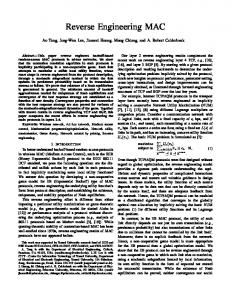
Figure 1. Data acquisition (upper left), registration (right) and mesh reconstruction (lower left) for the head of an antique statue.1 During the last few years we developed a nearly automatic processing pipeline covering the complex task from gathering data by an optical 3-D sensor to generating meshes of triangles. The whole surface of an object can be obtained by registering range images taken from arbitrary positions. The procedure includes the following steps (see Fig. 1): 1. Data acquisition: Usually multiple range images of one object are taken to acquire the whole object surface. These images consist of coordinate triples (x, y, z) arranged in a matrix, as on the CCD chip of the camera. 1 The original color images can be viewed in “www.optik.unierlangen.de/osmin/haeusler/people/sbk/papers/3dim2001_algo.pdf”.

2. Surface registration: The various views are transformed into a common coordinate system and are aligned to each other. First, the surfaces are interactively and coarsely aligned by pairs. Then, an ICP algorithm [1] minimizes the remaining deviations between all the views. 3. Mesh reconstruction: The views are merged into a single object model. A surface description is generated using a mesh of curved triangles. The order of the original data is lost, resulting in “scattered” data. 4. Data modeling and smoothing: A new modeling method for triangle meshes allows to interpolate curved surfaces only from the vertices and the vertex normals of the mesh. Using curvature dependent mesh thinning it provides a compact description of the curved triangle meshes. Measurement errors, such as sensor noise, aliasing, calibration and registration errors, can be eliminated without ruining the object edges. 5. Color reconstruction: For each range image a congruent normalized texture map is computed. In order to eliminate artifacts caused by illumination effects, two images of the same object view with illumination from different directions are merged. In this paper we will discuss the items “mesh reconstruction” and “data modeling and smoothing”. We will show some results that were modeled with our software system2 SLIM3D .

2 Related Work 2.1 Mesh Reconstruction Volumetric approaches have been used most frequently in recent years to reconstruct the topology of an object from a cloud of sampled data points. These are based on well established algorithms of computer tomography like marching cubes and therefore are easily implemented. They produce approximated surfaces, so that error smoothing is carried out automatically. The method of Hoppe et al. [5] is able to detect and model sharp object features but allows the processing of some 10,000 points only. Curless and Levoy [3] can handle millions of data points, but only matrix like structured range images can be used. Levoy et al. [9] used this reconstruction method for their impressive “Digital Michelangelo Project”.3 The usage of topology information provided by the range images enables faster algorithms and more accurate results. For that reason, Turk and Levoy [12] have proposed 2 www.optik.uni-erlangen.de/osmin/slim_e.html 3 www-graphics.stanford.edu/projects/mich/

a method for merging multiple range images into a single triangular mesh. While their “Mesh Zippering” algorithm solely stitches the boundaries of overlapping regions, our approach merges the meshes completely. In contrast to volumetric methods, merging techniques can generate interpolating meshes and therefore yield — in theory — more accurate results. On the other hand, special efforts for smoothing of measurement errors are required.

2.2 Data Modeling and Smoothing Calibration and registration errors usually appear after merging multiple range images from different views. Triangle meshes are so-called “unstructured grids” [13] and therefore it is not possible to use conventional modeling or signal processing methods like tensor product surfaces or linear filters. Unfortunately, no basic theory exists for handling unstructured data in order to estimate surface normals and curvature, interpolate curved surfaces, and subdivide or smooth triangle meshes. Merely, some limited approaches exist that work for special cases. Multiresolution analysis based on wavelets can only be used for triangle meshes with subdivision connectivity4 [10]. An approach for general meshes was proposed by Taubin [11]. He has generalized the discrete Fourier transformation by interpreting frequencies as eigenvectors of a discrete Laplacian. Defining such a Laplacian for irregular meshes allows to use linear signal processing tools like high and low pass filters, data compression and multiresolution hierarchies. However, the translation of concepts of linear signal theory is not the optimal choice for modeling geometry data. Surfaces of three-dimensional objects usually consist of segments with low bandwidth and transients with high frequency between them. They have no “reasonable” shape, as it is presupposed for linear filters. “Optimal” filters like Wiener or matched filters usually minimize the root mean square (RMS) error. Oscillations of the signal are allowed, if they are small. For visualization or milling of surfaces, curvature variations are much more disturbing than small deviations from the ideal shape. A smoothing filter for geometric data should therefore minimize curvature variations. Therefore we have generalized the Laplacian approach for invariance of surfaces with constant curvature. So did Desbrun et al. [4]. However, while they have defined their “curvature flow” operator heuristically, our “circular arcs” approach [7] is inspired by physical observations. Our method works best with dense meshes like those reconstructed from range images. Since it requires topological information, it is necessary to triangulate pure point clouds in advance. 4 All vertices (with singular exceptions) have the same number of neighbors.

tex insertion, gap bridging and mesh growing (see Fig. 3). Initially, a master image is chosen. The other views are merged into it successively. Only those vertices are inserted which do not cause any topological artifacts5 (e. g., flipped triangles) and which are required to keep the approximation error below a given threshold. 5. Final smoothing: Due to calibration and registration errors the meshes do not match perfectly. Thus, after merging the mesh is usually distorted and has to be smoothed again.

Figure 2. Thinned mesh of a technical object with curvature dependent density. The permitted approximation error in highly curved areas is less than in areas with low curvature (compare with Fig. 5).

3 Mesh Reconstruction The object surface is reconstructed from multiple registered range images. If the sensor is calibrated, the images consist of a matrix of coordinate triples xn,m = [x, y, z]Tn,m . The object surface may be sampled incompletely and the sampling density may vary, but should be as high as possible. Beyond that, the object may have arbitrary shape, and the field of view may even contain several objects. The following steps are performed to turn these data into a single mesh of curved or flat triangles: 1. Mesh generation: Because of the matrix-like structure of the range images, it is easy to separately turn each of them into triangle meshes with the data points as vertices. For each vertex a normal is calculated from the normals of the surrounding triangles. 2. First smoothing: In order to utilize as much of the sampled information as possible, smoothing of measurement errors like noise and aliasing is done before mesh thinning. 3. First mesh thinning: Merging dense meshes usually requires too much memory, so that mesh reduction must be carried out in advance. The permitted approximation error should be chosen as small as possible, as ideally thinning should be done only at the end of the process pipeline. Figure 2 shows a thinned mesh with curvature dependent density. 4. Merging: The meshes from different views are merged by pairs using local mesh operations like ver-

6. Final mesh thinning: Mesh thinning is continued until the given approximation error is reached. For thinning purposes also a classification of the surfaces according to curvature characteristics is carried out (see Fig. 5). 7. Closing of holes and gaps: Usually, data are missing due to shadowing effects or because it is not possible to acquire the complete surface of the object. This causes holes and gaps in the reconstructed mesh which are filled with flat triangles. The new triangles are refined by a new subdivision scheme to seemlessly integrate them into the measured data [8].6 8. Geometrical mesh optimization: Thinning usually causes awkward distributions of the vertices, so that elongated triangles occur. Geometrical mesh optimization moves the vertices along the curved surface in order to produce a better balanced triangulation.7 9. Topological mesh optimization: Finally, the surface triangulation is reorganized using edge swap operations, in order to optimize certain criteria. Usually, the interpolation error is minimized. The result of this process is a mesh of curved triangles. A new modeling method is able to interpolate curved surfaces solely from the vertex coordinates and the assigned normal coordinates. This enables a compact description of the mesh, as modern data exchange formats like Wavefront OBJ, Geomview OFF, Metastream MTS, or VRML support this data structure.

4 Modeling of Dense Triangle Meshes Many of the errors that are caused by the measuring process (noise, aliasing, outliers, etc.) can be filtered at the 5 Since vertex insertion is carried out in direction of the vertex normals, the probability for generating artifacts is minimized. 6 See file “subdivision_d.html” in folder “www.optik.uni-erlangen.de/osmin/haeusler/people/sbk/”. 7 See “Interpolation_d.html” in the same folder.

Figure 5. An application of curvature estimation. The vertices of the mesh of Fig. 2 are color coded according to their curvature characteristics (red = flat, green = cylindrical convex, blue = cylindrical concave, magenta = convex, yellow = concave, cyan = saddle). Figure 3. Merging of two meshes using vertex insertion, gap bridging, and mesh growing operations (projection in normal direction).

Figure 4 shows a cross section S with arc length si j through a constantly curved object surface between two adjacent vertices Vi and Vj . The curvature ci j of the curve S is (ci j > 0 for concave and ci j < 0 for convex surfaces) αi j αi j arccos(~ni ·~n j ) 1 ≈± ≈± , ci j = ± = ± r si j di j di j

Figure 4. Cross section S through a constantly curved surface. level of raw sensor data. A special class of errors (calibration and registration errors) first appears after merging the different views. We use a new modeling method that is based on the assumption, that the underlying surface can be approximated by circular arcs [7]. This algorithm allows the elimination of measuring errors without disturbing object edges and the interpolation of curved surfaces (e.g., curved triangles) which is simply done by interpolation between the circular arcs [8].8 It is assumed that the triangle mesh approximates a smooth surface with the vertices as sampled surface points. The sampling density ought to be high enough to neglect the variations of surface curvature between adjacent vertices. If this is true, the underlying surface can be locally approximated by circular arcs. As an example we show how easy curvature estimation can be done when this simplified model is used. 8 See

“Interpolation_d.html”.

(1)

which can be easily computed if the surface normals~ni and ~n j are known (they can be computed from the normals of the triangles meeting at Vi ). The principal curvatures κ1 (i) and κ2 (i) of Vi are the extreme values of ci j with regard to all its neighbors Vj : κ1 (i) ≈ min(ci j ) and κ2 (i) ≈ max(ci j ). j

j

(2)

The surface normals are computed separately, hence it is possible to eliminate noise by smoothing the normals without any interference of the data points. Therefore, this method is much less sensitive to noise than the usual method for curvature estimation from sampled data which is based on differential geometry [2]. Jain and Ittner [6] heuristically introduced a simplified ||~n −~n || approximation for Eq. (1): ci j ≈ idi j j . Our modeling method now proves that their measure is a good curvature estimation for dense meshes. Figure 5 demonstrates an application of this curvature estimation method. The vertices of the mesh of Fig. 2 are color coded according to their curvature properties.

5 Smoothing Triangle Meshes Filtering is done by first smoothing the vertex normals of the mesh and then using a non-linear geometry filter to adapt the positions of the vertices.

Figure 6. Cross section S through a constantly curved surface. The position of vertex V is not measured correctly. The “circular arcs approach” is used for smoothing measurement errors with minimum interference on real object features like edges. If curvature variations of the sampled surface are actually negligible, while the measured data vary from the approximation of circular arcs, this must be caused by measuring errors. Therefore, it is possible to smooth these errors by minimizing curvature variations. For this purpose a measure δ is defined to quantify the variation of a vertex from the approximation model. Figure 6 shows a constellation similar to Fig. 4. Now the vertex V is measured at a wrong position. The correct position would be V0i if Vi and the surface normals~n and~ni perfectly match the simplified model (there exist different ideal positions V0i for each neighbor Vi ). The deviation of V with regard to Vi , given by δi ≈ d i

cos(βi − α2i ) , cos( α2i )

(3)

can be eliminated by translating V into V0i . For regular meshes (di ≈ const ∀ i) the sum over δi defines a cost function for minimizing the variations of V from the approximation model. Minimizing all cost functions of all vertices simultaneously leads to a mesh with minimum curvature variations for fixed vertex normals. Alternatively it is possible to define a recursive filter for general meshes by repeatedly moving each vertex V along its assigned normal~n by ∆n =

1 N 1 < δi > := wi δi , 2 2N ∑ i

(4)

where N is the number of neighbors of V and wi are weights that attenuate the influences of the Vi according to their distances di : wi =

d0 . di

(5)

d0 is the minimum distance between all vertices of the mesh (usually the sampling distance). Weighting is necessary,

Figure 7. Smoothing of an idealized registration error on a flat surface. After moving each vertex by ∆n = 12 < δi > along its normal vector, the data points are placed in the fitting plane of the original data. since otherwise far away vertices would have more importance than contiguous ones. Using curvature dependent weights, it is possible to preserve or even enhance edges while smoothing.9 After a few iterations all ∆n converge towards zero and the overall deviation of all vertices from the circular arc approximation reaches a minimum. Restricting the translation of each vertex to only a single degree of freedom (direction of the surface normal) enables smoothing without seriously affecting small object details (compare with Turk and Levoy [12]). Conventional approximation methods, in contrast, cause isotropic daubing of delicate structures.

5.1 Smoothing of Calibration and Registration Errors This procedure can be used for surface smoothing if the surface normals describe the sampled surfaces more accurately than the data points. In case of calibration and registration errors the previous assumption is realistic. This class of errors usually causes local displacements of the overlapping parts of the surfaces from different views, while any torsions are locally negligible. Oscillating distortions of the merged surface with nearly parallel normal vectors at the sample points are the result. Figure 7 shows an idealization of such an error if the sampled surface is flat. The jagged line of vertices derives from different images that were not perfectly registered. It is clear that this error can be qualitatively eliminated, if the vertices are forced to match the 9 See

“smoothing2_d.html”.

Figure 8. Distorted mesh of a human tooth, reconstructed from 7 badly matched range images (left), and the result of smoothing (right).

defaults of the surface normals by translating each vertex by Eq. (4) along its normal. If the sampled surface is flat, the resulting vertex positions are placed in the fitting plane of the original data points. In case of curved surfaces, the regression surfaces are curved too, with minimum curvature variations for fixed surface normals. This method generalizes standard methods for smoothing calibration and registration errors by locally fitting planes to the neighborhood of each vertex [5, 12]. Instead of fitting piecewise linear approximation surfaces, in our case surface patches with piecewise constant curvature are used. Figure 8 demonstrates that registration and calibration errors in fact can be smoothed without seriously affecting any object details. The mesh on the left side of Fig. 8 is reconstructed from 7 badly matched range images of a human tooth. The mean registration error is 0.14 mm, the maximum is 1.5 mm (19 times the sampling distance of 0.08 mm!). The mean displacement of a single vertex by smoothing is 0.06 mm, the maximum is 0.8 mm. The displacement of the barycenter is 0.002 mm. This indicates that the smoothed surface is perfectly placed in the center of the difference volume between all range images.

Figure 9. Noisy range image of a ceramic bust (left), smoothed by a 7 × 7 median filter (center), and by the described smoothing method (right).

edge preserving filters. Although the errors (variations of the smoothed surface from the original data) of the median filter are slightly larger in this example, the described smoothing method shows much more noise reduction. Beyond that, the median filter produces new distortions at the boundaries of the surface. The new smoothing filter reduces the noise by a factor of 0.07, whereas the median filter actually increases the noise because of the produced artifacts. The only disadvantage of smoothing is a nearly invisible softening of small details. Experiments showed that the errors introduced by smoothing are always less than the errors of the original data. In particular no global shrinkage, expansion or displacement takes place, a fact that is not self-evident when using real 3-D filters.

6 Results 5.2 Smoothing of Noise and Moiré In case of noise or aliasing errors (Moiré) the surface normals are also distorted, but can simply be smoothed by weighted averaging. Thus filtering is done by first smoothing the normals (normal filter) and then using the described geometry filter to adapt the positions of the data points to these defaults. Figure 9 demonstrates smoothing of measuring errors of a single range image in comparison to a conventional median filter, which is the simplest and most popular type of

The described mesh reconstruction method was tested with many different objects, technical and natural as well. The following examples were digitized by our sensors and reconstructed with our SLIM3D software. Figure 10 shows the results for a design model of a firefighter’s helmet. The reconstructed CAD data are used to produce the helmet. For that purpose, the triangular mesh was translated into a mesh of Bézier triangles, so that small irregularities on the boundary could be cleaned manually. This work was carried out in collaboration of the Chair for

Figure 10. Reconstructed mesh of a firefighter’s helmet (left) and the helmet that was produced from the CAD data (right). Figure 12. Reconstruction of the head of St. George: rendered with plain surface (left) and with colored vertices (right).

Figure 11. Reconstructed surfaces of plaster models of a human canine tooth (left: 35,642 triangles, 870 kB) and a molar (right: 64,131 triangles, 1.5 MB).

Optics and the Computer Graphics Group10 of the University of Erlangen. Eight range images containing 874,180 data points (11.6 MB) were used for surface reconstruction. The standard deviation of the sensor noise was 0.03 mm (10% of the sampling distance), the mean registration error was 0.2 mm. On a machine with an Intel Pentiumr II 300 processor, the surface reconstruction took 7 minutes allocating 22 MB of RAM. The resulting surface consists of 33,298 triangles (800 kB) and has a mean deviation of 0.07 mm from the original (unsmoothed) range data. For a virtual catalogue of teeth for medical applications we measured a series of 26 human plaster tooth models of twice the natural size. Figure 11 shows a reconstructed canine tooth and a molar. Ten views (15 resp. 13 MB) were processed. Surface reconstruction took 6 resp. 7 minutes. 10 www9.informatik.uni-erlangen.de

For the “Germanisches Nationalmuseum” in Nürnberg we measured parts of a statue of Saint George (15th Century). The results are planned to enable a “virtual” restoration of the statue. Moreover, the 3-D data allow to distinguish between relief and painted structures (texture) of the surface. For the visitors of the museum it will be interesting to watch a 3-D simulation of the restoration process. Moreover, the obtained 3-D model enables to view the statue in a virtual (e. g., ancient) environment. The 3-D measurements were done using a phase measuring triangulation (pmt) sensor. Since the statue is partially very dark (e. g., the hair), 16 measurements for each view were overlayed. Nevertheless, some sections of the surface could not be measured. These missing data were automatically reconstructed by our new subdivision method [8].11 For each of altogether 26 views a normalized texture map was reconstructed. This was used to color the vertices of the final mesh (Fig. 12). In order to avoid loss of detail, mesh thinning was carried out very carefully. The final mesh consists of 400,000 triangles. Hence, surface reconstruction took 6 hours. The final mesh approximates the raw sensor data with a mean deviation of 140 µm. The last example demonstrates how a hardcopy of an angel from the “Bamberger Dom” was made without touching the damageable work of art. 200 range images were taken in order to acquire the whole surface of the statue. Since the memory of the used machine (1 GB) was not sufficient to merge all images into a single mesh, the data was cut into five slices which were processed separately and merged after the final mesh thinning. The resulting mesh consists of 1,450,000 triangles and was used to manufacture a copy in ABS plastics. From this a casting in a stone-like material was made. The whole process took approx. 2 months. 11 See

“closing_d.html”.

References

Figure 13. Making of a hardcopy of an angel from the “Bamberger Dom” (left: the original statue made of sandstone, middle: triangle mesh reconstructed from 200 range images, right: replica made of ABS plastics.

7 Conclusions We have presented an almost automatic pipeline for digitizing the complete surface of an object and for reconstructing a triangular mesh with high accuracy for metrology purposes. Sensor noise, and calibration, and registration errors are smoothed without significant loss of details. The errors reinduced by the modeling process are usually smaller than the errors in the original data (measuring, calibration, and registration errors). The smoothing method is specifically adapted to the requirements of geometric data, as it minimizes curvature variations. Undesirable surface waviness is avoided. Surfaces of high quality for visualization, NC milling and “real” reverse engineering are reconstructed. The user defines a limit for the approximation error which determines the density of the final mesh. Small holes and gaps due to missing data are automatically closed and seemlessly interpolated. Normally, no manual post-processing is required.

Acknowledgement Parts of this work were supported by the “Deutsche Forschungsgemeinschaft” (DFG #1319/8-4 and SFB 603) and by the “Studienstiftung des deutschen Volkes”.

[1] P. Besl and N. McKay. A method for registration of 3-d shapes. IEEE Transactions on Pattern Analysis and Machine Intelligence, 14(2):239–256, Feb. 1992. [2] P. J. Besl and R. C. Jain. Invariant surface characteristics for 3d object recognition in range images. Computer Vision, Graphics, and Image Processing, 33:33–80, 1986. [3] B. Curless and M. Levoy. A volumetric method for building complex models from range images. In H. Rushmeier, editor, SIGGRAPH 96 Conference Proceedings, pages 303– 312. Addison Wesley, Aug. 1996. [4] M. Desbrun, M. Meyer, P. Schröder, and A. H. Barr. Implicit fairing of irregular meshes using diffusion and curvature flow. In A. Rockwood, editor, Proceedings of SIGGRAPH 99, pages 317–324. Addison Wesley, Aug. 1999. [5] H. Hoppe, T. DeRose, T. Duchamp, J. McDonald, and W. Stuetzle. Surface reconstruction from unorganized points. In E. E. Catmull, editor, Computer Graphics (SIGGRAPH ’92 Proceedings), volume 26, pages 71–78, July 1992. [6] A. K. Jain and I. D. J. Segmentation of range images. In Proceedings of the First Annual Artificial Intelligence & Advanced Computer Technology Copnference, pages 23–28, 1985. [7] S. Karbacher. Discrete modeling of point clouds. In B. Girod, G. Greiner, and H. Niemann, editors, Principles of 3D Image Analysis and Synthesis, pages 166–175. Kluwer Academic Publishers, Boston-Dordrecht-London, 2000. [8] S. Karbacher, S. Seeger, and G. Häusler. A non-linear subdivision scheme for triangle meshes. In B. Girod, H. Niemann, and H.-P. Seidel, editors, Vision, Modeling and Visualization 2000, pages 163–170. Akademische Verlagsgesellschaft, Berlin, 2000. [9] M. Levoy, K. Pulli, B. Curless, S. Rusinkiewicz, D. Koller, L. Pereira, M. Ginzton, S. Anderson, J. Davis, J. Ginsberg, J. Shade, and D. Fulk. The digital michelangelo project: 3D scanning of large statues. Proceedings of SIGGRAPH 2000, pages 131–144, July 2000. [10] M. Lounsbery, T. D. DeRose, and J. Warren. Multiresolution analysis for surfaces of arbitrary topological type. ACM Transactions on Graphics, 16(1):34–73, Jan. 1997. [11] G. Taubin. A signal processing approach to fair surface design. In R. Cook, editor, SIGGRAPH 95 Conference Proceedings, pages 351–358. Addison Wesley, Aug. 1995. [12] G. Turk and M. Levoy. Zippered polygon meshes from range images. In A. Glassner, editor, Proceedings of SIGGRAPH ’94 (Orlando, Florida, July 24–29, 1994), pages 311–318. ACM Press, July 1994. [13] R. Westermann. Volume models. In B. Girod, G. Greiner, and H. Niemann, editors, Principles of 3D Image Analysis and Synthesis, pages 245–251. Kluwer Academic Publishers, Boston-Dordrecht-London, 2000.