PV Power Output Variability: Correlation Coefficients

PV Power Output Variability: Correlation Coefficients Thomas E. Hoff and Richard Perez Clean Power Research www.cleanpower.com Draft, November 11, 2010

Abstract Utility planners and operators are responsible for guiding where PV systems are located and are accountable for system reliability. They are concerned about how short‐term PV system output changes may affect utility system stability. That is, they are concerned about PV power output variability. This paper introduces a novel approach to estimate the maximum short‐term output variability that a fleet of PV systems places on any considered power grid. A key input to this approach is the correlation, or absence thereof, existing between individual installations in the fleet at the considered variability time scale. Short‐term PV power output variability is driven by changes in the clearness index. Thus, the paper focuses on analyzing the correlation coefficient of the change in the clearness index between two locations as a function of distance, time interval, and other parameters. The paper presents a method to estimate correlation coefficients that uses location‐specific input parameters. The method appears to be capable of describing site‐pair correlation across time intervals from seconds to hours. The method is derived empirically and validated using 12 years of hourly satellite‐derived data from SolarAnywhere® in three geographic regions in the United States (Southwest, Southern Great Plains, and Hawaii). Results at time intervals less than one hour are corroborated using findings from recent investigations that were based on 10‐second to one‐minute data sets. The strength and structure of the method is summarized by three fundamental findings that both confirm and extend conclusions from previous studies: 1. Correlation coefficients decrease predictably with increasing distance. 2. Correlation coefficients decrease at a similar rate when evaluated versus distance divided by the considered variability time interval. 3. The accuracy of results is improved by including an implied cloud speed term. The present approach has potential financial benefits to systems that are concerned about PV power output variability, ranging from distribution feeders to balancing regions.

Copyright © 2010 Clean Power Research

1

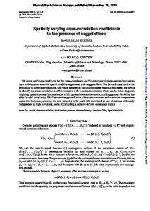
Introduction PV capacity is increasing on utility systems. As a result, utility planners and operators are growing more concerned about potential impacts of power supply variability caused by transient clouds. Utilities and control system operators need to adapt their planning, scheduling, and operating strategies to accommodate this variability while at the same time maintaining existing standards of reliability. It is impossible to effectively manage these systems, however, without a clear understanding of PV output variability or the methods to quantify it. Whether forecasting loads and scheduling capacity several hours ahead or planning for reserve resources years into the future, the industry needs to be able to quantify expected output variability for fleets of up to hundreds of thousands of PV systems spread across large geographical territories. Underestimating reserve requirements may result in a failure to meet reliability standards and an unstable power system. Overestimating reserve requirements may result in an unnecessary expenditure of capital and higher operating costs. The present objective is to develop analytical methods and tools to quantify PV fleet output variability. Variability in time intervals ranging from a few seconds to a few minutes is of primary interest since control area reserves are dispatched over these time intervals. For example, regulation reserves might be dispatched at an ISO every five seconds through a broadcast signal. Knowledge about PV fleet variability in five‐second intervals could be used to determine the resources necessary to provide frequency regulation service in response to power fluctuations. Variability of a PV fleet is thus a measure of the magnitude of changes in its aggregate power output corresponding to the defined time interval and taken over a representative study period. Note that it is the change in output, rather than the output itself, that is desired. Also note that, for each time interval the change in output may vary in both magnitude and sign (positive and negative). A statistical metric is therefore employed in order to quantify variability: the standard deviation of the change in fleet power output. It is helpful to graphically illustrate what is meant by output variability. The left side of Figure 1 presents 10‐second irradiance data (PV power output is almost directly proportional to irradiance) and the right side of the figure presents the change in irradiance using a 10‐second time interval for a network of 25 weather monitoring stations in a 400‐meter by 400‐meter grid located at Cordelia Junction, CA on November 7, 2010 (Hoff and Norris, 2010). The light gray lines correspond to irradiance and variability for a single location and the dark red lines correspond to average irradiance distributed across 25 locations. Results suggest that spreading capacity across 25 locations rather than concentrating it at a single location reduces variability by more than 70 percent in this particular instance.


2

work reducess 10‐second vvariability by m more than 70 0 percent in aa 400 Figure 1. Twenty‐five location netw mete er x 400 meter grid at Cord delia Junction , CA on Noveember 7, 2010 0.

A “fleet co omputation” approach can n be taken to o calculate outtput variabilitty for a fleet of PV systems as follows: id dentify the PV V systems thaat constitute tthe fleet to b e studied; select the time interval and time period of concern (e.g.., one‐minute e changes evaaluated over aa one‐year peeriod); obtain n time‐ put synchroniized solar irraadiance data ffor each locattion where a PV system is to be sited; ssimulate outp for each P PV system using standard m modeling too ols; sum the ooutput from eeach individuaal system to obtain the e combined fleet output; ccalculate the change in fle et output forr each time in nterval; and finally calculate the resulting statistical ou utput variability from the sstream of valu ues. This “fleett computation” approach, while technically valid, is difficult to im mplement in p practice for several re easons. First, insolation datta is not availlable in sufficcient resolutio on (either tim me resolution or geographical resolution). For examp ple, SolarAnywhere (2010)), which provvides operatio onal real‐timee n data for the continental U U.S. and Haw waii, is currenttly based on aa 10 km x 10 km grid and aa one‐ insolation hour time e interval. It h has a practical real‐time lim mit of one‐hallf hour and a few km baseed on current satellite te echnology. Fleet computation could no ot be perform med for, say, ssystems spaceed 0.5 km apaart with a fou ur‐minute tim me interval. Se econd, PV varriability deterrmined using the fleet com mputation approach is only appliccable to studies having a m matching timee interval of interest and aa fixed fleet onal PV system ms came on‐line. selection. The study would have to be re‐commissioned whennever additio e highly comp putation inten nsive, and thuus are not suiitable for real‐time operattions. Finally, caalculations are A more viable approacch is to stream mline the calcculations throough the use o of a general‐p purpose PV output variabilityy methodologgy. The method needs to q quantify shortt‐term fleet p power outputt variability using the observations that ssky clearness and sun posiition drive thee changes in tthe short‐term output for individuall PV systems aand that physsical parametters (i.e., dimeensions, plan nt spacing, number of plants, etc.) determine overall fleet variabiility. Hoff and P Perez (2010) developed a simplified mo odel as a firstt step towards a general m method to quaantify the outpu ut variability rresulting from m an ensemble of equally‐sspaced, identtical PV system ms. They defiined Copyrightt © 2010 Cleaan Power Research

3

output variability to be the standard deviation of the change in output over some time interval (such as one minute), using data taken from some time period (such as one year). The simplified model covered the special case when the change in output between locations is uncorrelated (i.e., cloud impacts at one site are too distant to have predictable effects at another for the considered time scale), fleet capacity is equally distributed, and the variance at each location is the same. Under these conditions, Hoff and Perez showed that fleet output variability equals the output variability at any one location divided by the square root of the number of locations:1

√

( 1 )

where is the standard deviation of the change in output of the fleet using a time interval of Δt, is the standard deviation of the change in output of the fleet concentrated at a single location, and N is the number of uncorrelated locations. Mills and Wiser (2010) have derived a similar result that relates variability to the square root of the number of systems when the locations are uncorrelated.

Maximum Output Variability Equation ( 1 ) has important implications for utility planners. It allows them to determine reserve capacity requirements to mitigate worst case fleet variability. For example, suppose that the variability of a single system was 10 kW per minute and there were 100 uncorrelated identical systems in the fleet. Total fleet variability equals 0.1 MW (

∗ √

per minute. The planner could then apply the desired

confidence level (e.g., they may choose 3 standard deviations) to determine the required reserve capacity (e.g., 3 x 0.1 MW = 0.3 MW). This calculation is applicable when two fundamental conditions are satisfied: (1) the output variability at a single location can be quantified and (2) the change in output variability between locations is uncorrelated. Consider the first condition. One approach to determining single location variability ( ) is to analyze historical solar resource data for the location of interest. The data would need to have been collected at a rate that accommodates the time interval of interest (perhaps down to a few seconds) over a substantial and representative period of time (perhaps over several years). Such high‐speed, high‐ resolution data is not generally available.2 An alternative approach is to construct a data set that simulates worst case variability conditions. The theoretically worst case variability of a single PV plant would be that it cycles alternately between 0 and 100 percent of its rated output every time interval. For example, suppose that the PV plant is rated at 1

1 2

See Equation (8) in Hoff and Perez (2010). One of the few examples of this sort of data is provided by Kuszamaul, et. al. (2010).


4

MW and the time interval of interest is 1 minute. As illustrated in Table 1, maximum variability occurs when the PV plant is at full power at 12:00, zero power at 12:01, full power at 12:02, etc. As illustrated in the right side of the table, the corresponding change in power fluctuates between ‐1 and 1 MW. The standard deviation3 of the change in power output equals 1 MW per minute. That is, a 1 MW PV plant that is exhibiting maximum variability over a 1 minute time interval has a 1 MW per minute standard deviation. This would imply that 1 MW of reserve capacity is required to compensate for the output variability for a single plant.

Table 1. Maximum change in power output at one location. Time 12:00 12:01 12:02 12:03 12:04

Power (MW) 1 0 1 0 1

Change (MW/min) ‐1 +1 ‐1 +1

Suppose that the PV “fleet” capacity was split between two locations and each were to exhibit maximum output variability. Two possible scenarios exist. The first scenario, illustrated in Table 2, assumes that both plants turn on and off simultaneously. As was the case where all capacity is concentrated at a single location, the change in output fluctuates between ‐1 and 1 MW and the standard deviation for this scenario is 1 MW per minute. The second scenario, illustrated in Table 3, assumes that the plants cycle on and off alternately with a time shift of 1 minute. In this case, the change in output from the first location cancels the change in output at the second location. The result of this scenario is a standard deviation of 0 MW per minute. It is incorrect to conclude, however, that the upper bound of output variability for 1 MW of PV is 1 MW per minute because this is the larger value of the two scenarios (the first equals 1 MW per minute and the second equals 0 MW per minute). This is because each of the two scenarios violates the assumed condition that the locations are uncorrelated. Specifically, the change in output between the two locations has perfect positive correlation in the first scenario (i.e., correlation coefficient equals 1) and perfect negative correlation in the second scenario (i.e., correlation coefficient equals ‐1).

3 The standard deviation of a random variable X equals the square root of the expected value of X squared minus the square of the expected value of X. σ

EX

E X .


5

Table 2. Maximum change in power output at two locations (scenario 1). Time 12:00 12:01 12:02 12:03 12:04

Power (MW) Plant 1 0.5 0 0.5 0 0.5

Change (MW/min) Fleet (1+2) 1 0 1 0 1

Plant 2 0.5 0 0.5 0 0.5

‐ 1 +1 ‐1 +1

Table 3. Maximum change in power output at two locations (scenario 2). Time 12:00 12:01 12:02 12:03 12:04

Plant 1 0.5 0 0.5 0 0.5

Power (MW) Plant 2 Fleet 1+2 0 0.5 0.5 0.5 0 0.5 0.5 0.5 0 0.5

Change (MW/min) 0 0 0 0

Feasible Maximum Output Variability These scenarios demonstrate that it is impossible for two systems to exhibit the behavior of worst case variance individually (by cycling on and off at each interval) without having either perfect positive or perfect negative correlation. Indeed, for each system to exhibit its maximum variance, its output changes must be exactly in tempo with the time interval, loosely analogous to each member of an orchestra following in time to its conductor, in which case the systems would by definition have perfect correlation (whether positive or negative). By this reasoning, the maximum output variability scenario described above (1 MW of variability for each 1 MW of fleet capacity) is impossible. When the systems have less than perfect correlation, as must be the case for any real‐world fleet, the variability of the combined fleet must be less than the total fleet capacity. To correct the worst case scenario, retain the assumption that each power change is either a transition from zero output to full output or from full output to zero output. This assumption in itself is highly conservative since the impacts of cloud transients on PV systems will almost never produce changes with magnitudes as high as 100 percent of rated output and will generally produce changes much less than 100 percent. As for timing, rather than being synchronized, each system is assumed to cycle on and off in a random fashion, representing fleets of PV systems with outputs that are uncorrelated. Random timing of power output changes is illustrated for a single location in Table 4 for a 1 MW PV system. Suppose that it is 12:00 and the time interval is 1 minute. There is a 50 percent chance that the Copyright © 2010 Clean Power Research

6

n and a 50 pe ercent chance e that the plan nt is off at 12 :00. If the plaant is on at 12 2:00, then theere is plant is on a 50 perce ent chance it will turn off aand a 50 perccent chance itt will remain on at 12:01. If the plant iss off at 12:00, tthen there is a 50 percent chance it willl stay off andd a 50 percentt chance it will turn on at 12:01. The e right colum mn in Table 4 p presents the p probability diistribution of the change in power. At eeach time interrval, there is aa 25 percent chance of a 1 1 MW per minnute decreasee in power, a 50 percent chance off no change in n output, and d a 25 percentt chance of a 1 MW per minute increasse in power. Note thatt while this is the maximum m possible change, it is exttremely unlikkely that such a distribution would acttually exist. Fiirst, weather conditions w would have to be exception nally erratic. SSecond, cloud ds would nee ed to be so dark that there e would be no o output wheen covering a PV system. TThird, the entire system would have to turn on and o off, rather thaan a subset oof the arrays. Fourth, each PV system w would Kuszamaul et.. al. (2010) an nd Mills et. al.. (2009) have need to operate as a “point source”” of output; K occurs as systeem size increases.4 demonstrrated that, in fact, a smootthing effect o Table e 4. Maximum m change in p power outputt assuming random outputt.

With thesse caveats, the above distrribution is takken for the cuurrent purposses. This distriibution has a standard deviation of times 1 MW W.5 If the enttire fleet of PV V systems weere concentraated at a singlle √

point, and d the fleet had a capacity o of CFleet, then the maximum m standard deeviation of ch hange in outp put equals:

( 2 )

2 √2 The maxim mum output vvariability forr a fleet of un ncorrelated loocations can b be calculated using this numerical definition off the maximu um output varriability for a single system m by substitutting Equation ( 2 ) into Equation ( 1 ).The result is thatt that maximu um output va riability equaals fleet capaccity divided by the square root of 2 times the number of uncorrelatted locations..

√2 √

( 3 )

4 5

See Figurre 13 in Kuszam maul et. al. (2010) and Figure 7 in Mills et. aal. (2009). 0.25 1 0.50 0 0.25 1 0.50 0 0.25 0 1

Copyrightt © 2010 Cleaan Power Research

0.25 1

√

7

n upper boun nd on the maxximum outpuut variability ffor any time in nterval as lon ng as Equation ( 3 ) places an between locattions is uncorrrelated. Actuual results aree likely to be lower. This the changge in output b practical u upper bound on single point output is substantiatedd by a wealth h of empirical evidence (seee Perez et aal., 2010a).

Examplle Suppose tthat a utility ssystem plans to incorporatte 5,000 MW of PV. Figuree 2 presents tthe maximum m output vaariability calcu ulated using EEquation ( 3 ) for PV fleets with capacitiies ranging from 0 to 5,000 0 MW based on two flee et composition strategies. The blue linee is the variab bility when thee fleet is d of uncorrelaated 1 MW syystems. The rred line is the variability when the fleett is composed d of composed uncorrelated 100 MW systems. As iillustrated in the figure at the 5,000 MW W level, if 100 0 MW system ms are ns (N=50) with h uncorrelate ed changes in output, maximum outputt variability iss 500 installed aat 50 location MW per ttime interval, or 10 percen nt of fleet cap pacity. Howevver, if 1 MW PPV systems arre installed att 5,000 locaations (N=5,0 000) with unco orrelated chaanges in outpuut, maximum m output variaability is 50 M MW, 6 or 1 perce ent of fleet caapacity. This exam mple illustrate es the potential benefit of dividing the PPV capacity in nto small systtems, and spreadingg them apart ggeographically so that outtput changes are uncorrelaated. More im mportantly, itt also illustratess the unnecesssary potentiaal cost that co ould be incurrred if system planners were to procuree reserves w without adequate tools for quantifying PV variabilityy. The dotted d line represeents the reserrve resourcess that would b be procured w when each MW of PV was fully “backed d up” with a M MW of fossil, battery, o or other dispaatchable resou urce. In the N N=5,000 exam mple, such a p planning pracctice — at least for fleets mad de up of unco orrelated systtems— would d result in cappital expendittures 99 timees the requireed amounts. Figure 2. Maximu um variability for 1 MW an nd 100 MW syystem sizes w with uncorrelaated changes..

6

Appendixx A illustrates h how to verify th hese results ussing an Excel sppreadsheet.


8

Correlation versus Distance Background: Critical Factors Affecting Correlation The critical factors that affect output variability are the clearness of the sky, sun position, and PV fleet orientation (i.e., dimensions, plant spacing, number of plants, etc.). To improve accuracy, Hoff and Perez (2010) introduced a parameter called the Dispersion Factor. The Dispersion Factor is a parameter that incorporates the layout of a fleet of PV systems, the time scales of concern, and the motion of cloud interferences over the PV fleet. Hoff and Perez demonstrated that relative output variability resulting from the deployment of multiple plants decreased quasi‐exponentially as a function of the generating resource’s Dispersion Factor. Their results demonstrated that relative output variability (1) decreases as the distance between sites increases; (2) decreases more slowly as the time interval increases; and (3) decreases more slowly as the cloud transit speed increases. Mills and Wiser (2010) analyzed measured one‐minute insolation data over an extended period of time for 23 time‐synchronized sites in the Southern Great Plains network of the Atmospheric Radiation Measurement (ARM) program. Their results demonstrated7 that the correlation of the change in the global clear sky index (1) decreases as the distance between sites increases and (2) decreases more slowly as the time interval increases. Perez et. al. (2010b) analyzed the correlation between the variability observed at two neighboring sites as a function of their distance and of the considered variability time scale. The authors used 20‐second to one‐minute data to construct virtual networks at 24 US locations from the ARM program (Stokes and Schwartz, 1994) and the SURFRAD Network and cloud speed derived from SolarAnywhere (2010) to calculate the station pair correlations for distances ranging from 100 meters to 100 km and from variability time scales ranging from 20 seconds to 15 minutes. Their results demonstrated that the correlation of the change in global clear sky index (1) decreases as the distance between sites increases and (2) decreases more slowly as the time interval increases. The consistent conclusions8 of these studies are that correlation: (1) decreases as the distance between sites increases and (2) decreases more slowly as the time interval increases. Hoff and Perez (2010) add that the correlation decreases more slowly as the speed of the clouds increases.

Objective Utility planners clearly require a tool that can reliably quantify the maximum output variability of PV fleets using a manageable amount of data and analysis. Equation ( 3 ) would potentially meet this requirement if the change in output between locations were uncorrelated (i.e., correlation coefficient is zero). In real fleets, PV systems will generally have some degree of correlation, so any planning tool will have to incorporate correlation effects in calculating actual fleet variability. This paper takes a step towards a general method by analyzing the correlation coefficient of the change in clearness index between two locations as a function of distance, time interval, and other parameters. 7 8

See Figure 5 in Mills and Wiser (2010). The results apply to either changes in PV output directly or changes in the clear sky index


9

It uses hourly global horizontal insolation data from SolarAnywhere (2010) to calculate correlation coefficients for 70,000 scenarios across three separate geographic regions in the United States (Southwest, Southern Great Plains, and Hawaii). The correlation coefficients taken from these scenarios are then compared to a method that could prove useful when integrated into utility planning and operations tool. Recognizing that the method must also be validated for shorter time intervals (several seconds to several minutes), its results are compared to studies based on 10‐second, 20‐second, and 1‐ minute insolation data sets.

Approach Hoff and Perez (2010) defined PV fleet variability as the standard deviation of its power output changes using a selected sampling time interval (e.g., such as one minute or one hour) and analysis period (such as one year), as expressed relative to the fleet capacity. To simplify the work, they formulated it in terms of the change in insolation rather than the change in PV power. As stated earlier, sky clearness and sun position drive the changes in short‐term output for individual PV systems. Mills and Wiser (2010) and Perez, et. al (2010) subsequently isolated the random component of output change and examined changes attributable only to changes in global clear sky (or clearness) index. The global clearness index equals the measured global horizontal insolation divided by the clear sky insolation. This paper continues in the direction of Mills and Wiser (2010) and Perez, et. al. (2010) and focuses on changes in the global clearness index.

Change in Global Clearness Index The global clearness index at a specific point in time is typically referred to as Kt*. It equals the measured global horizontal insolation (GHI) divided by the clear‐sky insolation. This paper refers to the change in the index between two points in time as ΔKt*. Since the change occurs over some specified time interval, Δt, at some specific location n, the variable is fully qualified as Δ ∗ , . This only represents one pair of points in time. A set of values is identified by convention by bolding the variable. ∗ Thus, is the set of changes in the clearness indices at a specific location using a specific time interval over a specific time period. ∗

,Δ

∗

,

,

,Δ

∗

,

,…,

∗

,Δ

,

( 4 )


10

Table 5 illustrates how to calculate the change in clearness index (ΔKt*) during conditions of rapidly changing insolation. For example, ΔKt* between 12:00 and 12:01 equals the difference between Kt* at 12:01 and Kt* at 12:00 (0.5 – 1.0 = ‐0.5). Table 5. Example of how to calculate change in clearness index (ΔKt*) using Δt = 1 minute. Time 12:00 12:01 12:02 12:03 12:04

GHI 1.0 0.5 0.0 0.5 1.0

Clear‐sky GHI 1.0 1.0 1.0 1.0 1.0

Kt* 1.0 0.5 0.0 0.5 1.0

ΔKt* ‐ 0.5 ‐ 0.5 +0.5 +0.5

Correlation and dependence in statistics are any of a broad class of statistical relationships between two ∗ ∗ or more random variables or observed data values (Wikipedia 2010). Let and represent two sets of observed data values for the change in the clearness index that have a mean of 0 and standard deviations, and . 9

Pearson’s product‐moment correlation coefficient (typically referred to simply as the correlation coefficient) equals the expected value of deviations. ∗

∗

times

∗

divided by the corresponding standard

∗

( 5 )

,

The analysis is performed as follows: 1. 2. 3. 4. 5. 6. 7. 8.

Select a geographic region for analysis Select a location for the first part of the pair Select a location for the second part of the pair Select a time interval for the analysis Select a clear sky irradiance level bin Obtain detailed insolation data Calculate the correlation coefficient 10 Repeat the calculation for all sets of location pairs, time intervals, and clear sky irradiance bins.

9 The expected value of ΔKt* equals 0 as long as the starting and ending GHI values are the same. This condition is satisfied when the time period of the analysis is performed over one day because the starting and ending GHI both equal 0. It will also be approximately true when the analysis encompasses many data points (as would be the case, for example, of an analysis of one hour of data using a one‐minute time interval). 10

Appendix B illustrates how to calculate ΔKt* correlation coefficients.


11

e if patterns eexisting that h help to betterr quantify The focuss of this paperr is on trying tto determine correlatio on coefficientss. As part of tthe objective,, a method is tested that p produces the desired output paramete er of the corre elation coefficcient of the change in the clearness ind dex between two separatee locations. As discussed d by Hoff and Perez (2010), the inputs innto this meth hod include th he distance between tthe two locattions, time intterval, and lo ocation‐speciffic parameterrs based on empirical weatther data, in particular, clou ud speed.

Resultss Scenariio Specificcation As summaarized in Table 6, three sep parate geograaphic regionss in the United d States weree selected forr analysis: SSouthwest, So outhern Greaat Plains, and Hawaii. The ffirst location (denoted by each of severral yellow squares in the ffigures), was sselected using a grid size oof 2.0°, 1.0°, o or 0.5° for thee Southwest, Southern Great Plains, and Hawaii, correspondin ngly. The secoond location ((denoted by aa red circle in n the figures) w was selected b between 0.1° and 2.9° (abo out 10 to 3000 km) from the first locatio on (other map p coordinattes were availlable but the illustrated po oints providedd sufficient data and ease of analysis, sso were igno ored). Hourly insolation daata was obtain ned for each of the two lo cations coverring the perio od January 1, 1998 througgh September 30, 2010 fro om SolarAnyw where (2010). The analysiss was then ed above for ttime intervalss of 1, 2, 3, annd 4 hours and for 10 sepaarate clear skyy performed as describe irradiance e bins. This an nalysis resulte ed in more than 70,000 coorrelation coeefficients. Table 6. Sum mmary of inp ut data. Region

Southwestt

Location # #1 Latitude:: 32° to 42°° Longitud de: ‐125° to ‐1 109° Grid Size e: 2.0° Location # #2 0.1°, 0.3°°, …, 1.9° from m #1 Time 1, 2, 3, and 4 hours Intervals Clear Sky 10 irradiance bins in intervals Irradiance e of 0.1 kW W/m2


Southern Great Plainss

Hawaii

Latitude: 335° to 38° Longitude: ‐999° to ‐96° Grid Size: 11.0° 0.1°, 0.3°, …, 2.9° from #11 1, 2, 3, and 44 hours

Latitude: 19° to 20° Longitu ude: ‐156° to ‐‐155° Grid Sizze: 0.5° 0.1°, 0.2°, …, 1.0° fro om #1 1, 2, 3, and 4 hours

10 irradiancee bins in increments oof 0.1 kW/m2

10 irrad diance bins in n incremeents of 0.1 kW W/m2

12

Correla ation Coeffficients Figure 3 p presents the ccorrelation co oefficients forr the Southweest.11 The collumns summarize the resu ults for each ttime interval aand the rows present the measured co rrelation coeefficients versus several alternativve candidate ssets of variables. The first column summ marizes resultts for a time iinterval of 1 h hour. The secon nd, third, and fourth colum mns plot the ssame results uusing time inttervals of 2, 3 3, and 4 hourss. Results in the top row present corre elation coefficients versuss the distancee between thee two location ns. oefficients verrsus distance divided by time interval. Results in the middle row present ccorrelation co oefficients veersus distancee divided by time interval Results in the bottom rrow present ccorrelation co 12 d by relative sspeed; this tterm is relate ed to the Disppersion Factorr introduced by Hoff and P Perez multiplied (2010). Th he dashed line e in the botto om figures represents the results of a ggeneralized m method, propo osed in this pap per for use in future tools,, that will be vvalidated in t he present an nalysis. Results are calculaated using paraameters obtaained from So olarAnywhere e. Figure 4 aand Figure 5 p present comp parative resultts for the Greeat Plains and d Hawaii. The patterns presented d in the figure es are similar across all tim me intervals inn the three geeographic loccations. Figuree 6 compressses the resultss for each location and pre esents resultss where all tim me intervals aare combined d into the same figure. Figure 3 3. Correlation n coefficients presented byy time intervaal for Southwest.

11

The dataa in all of the figures represen nt randomly se elected samplees of points in o order to make the results mo ore readable. 12 Relative speed equals tthe implied speed derived fo or the specific llocation from SSolarAnywheree data by the mplied speed accross the entire geographic rregion. Relativee speed is onlyy used for presentation purpo oses average im for the ben nefit of the reaader so that the e scale of the xx‐axis remains constant.


13

Figure 4. Correlation coefficients p presented by time interval for Great Plaains.

e 5. Correlatio on coefficientts presented by time interrval for Hawaii. Figure


14

Figu ure 6. Correlattion coefficients for all loccations and time intervals.

Discusssion The analyysis provides sseveral key fin ndings. First, consistent w ith previous sstudies, the ccorrelation coefficien nts decrease w with increasin ng distance (top row of Figgure 6). Secon nd, also consistent with previous sstudies, this d decrease occu urs more slow wly with longeer time intervvals (top row of Figure 6). An alternativve way of view wing this resu ult is that corrrelation coeffficients decrease at a similar rate when plotted ve ersus distance e divided by ttime interval (middle row of Figure 6). TThird, the scaatter in resultts is further de ecreased whe en a relative sspeed12 is intrroduced for thhe first locatiion in the pair of locationss (bottom rrow of Figure 6). Finally, th he generalize ed method, shhown by the d dashed black line in the bo ottom row of Figgure 6, fits the e empirical daata quite well when calibrrated using th he location‐sp pecific derived d input paraameters.

Resultss Project to o Shorter T Time Intervals An encouraging result of the forego oing analysis iis the ability oof the propossed general m method, validaated with several em mpirical data sets, to predict correlatio n coefficientss with such acccuracy. Even n directly w more encouraging is th hat the metho od is shown tto be valid reggardless of th he selected tim me interval. W While input dataa to the meth hod was taken n from the So olarAnywheree data set with a one‐hourr time interval, the method iss shown to prroduce accuraate correlatio on coefficientss for one‐hou ur, two‐hour, three‐hour, aand four‐hourr time intervals. This findin ng prompted tthe authors tto evaluate th he potential o of using the method b based on paraameters derivved from the SSolarAnywheere data set to o project resu ults to time intervals sshorter than o one hour.


15

be a highly valuable findingg if the metho od could be sshown to prod duce accuratee results for ttime It would b intervals sshorter than tthe available raw data. It would mean that the existing SolarAnyywhere data sset could be u used to deterrmine variabillity for fleets across the U..S., reducing tthe need for high‐speed, h high‐ resolution n data that is currently unaavailable. While the e desired obje ective is to de emonstrate th hat the methood accuratelyy determines correlation coefficien nts (and there efore variability) as a functtion of PV spaacing, a matheematically eq quivalent objeective is to show w that, for a given correlatiion coefficien nt, it is possibble to accurateely determinee spacing bettween PV system ms. The circles in Figure 7 ccorrespond to o the method d results take n from the do otted curve in n the bottom row of Figure 6. For example, Figure 6 im mplies that PV V systems ne ed to be spacced 40 km apart in the Greeat Plains in o order to achie eve a 25 perce ent correlatio on coefficientt using a 60 m minute time in nterval. Triplee the time interrval to 180 minutes and plants need to be spaced triiple the distance (120 km apart) to achieve the same 25 percent correlation coefficient. The solid lines connectting the four ttime interval observationss for each locaation in Figurre 7 illustrate that the relatio onship is lineaarly related to o the time intterval. The figgure begs thee question as to whether the results can be projecte ed in the regio on with shortter time intervvals (i.e., the gray sectionss of the figurees). Figure 7. Resu ults scale line early with the e time intervaal for a fixed ccorrelation co oefficient.

Evaluattion of Tim me‐Indepe endence Cllaim The above e linear relationship sugge ests that the m method is inddependent of selected time interval, evven down to tthe very shortt time intervaals (several se econds to sevveral minutes)) that are of p primary intereest to the utilitie es. This sectio on provides an initial validation of time ‐independence by comparing results calculated d from the on ne‐hour SolarA Anywhere daata set againstt results from m independen nt studies that used 10‐second, 20‐second, and one‐minute datta sets. Geographic Diversitty Study Mills and Wiser (2010)) used measured one‐minu ute insolationn data for 23 ttime‐synchro onized sites in n the Southern Great Plains network of th he Atmosphe eric Radiation Measuremen nt (ARM) pro ogram to


16

bility of PV with different d degrees of geeographic diveersity. That reeport presentted13 characterize the variab nges in global clear sky ind dex between tthese geographically dispeersed sites. M Mills the correllation of chan and Wiserr provided an n electronic ve ersion of their results and these were u used to comp pare against th he general m method propo osed here. Wh hile the one‐h hour SolarAnyywhere data set was used as input to th he general m method, correlation coefficcients were caalculated thatt correspondeed to much shorter time intervals iin the Mills an nd Wiser stud dy. The resultts, presented in Figure 8, aare comparab ble to the Millls and 14 Wiser study even down to one‐minute time intervals. Figure 8. Com F mparison of re esults to geoggraphic diverssity study.

Virtual N Network Stu udy Perez et. aal. (2010) obttained 20‐seccond to one‐m minute insolattion data for 24 measuringg stations, including 17 stations in n the ARM ne etwork and 7 stations in thhe SURFRAD n network. Theyy constructed d 15 5 ensional virtuaal networks using satellitte‐derived clooud speeds to o translate tim me measurem ments one‐dime into space e measureme ents. They then calculated d correlation ccoefficients b between the cchange in clearness index for varrious time inte ervals and disstances. Figurre 9 presentss some of the key results frrom that studyy. Figure 10 re e‐plots the daata from the vvirtual netwoork study alon ng with corressponding projection ns from the current study (based on inp put parameteers calculated d one‐hour So olarAnywheree data). Ressults compare e well to virtu ual network sttudy down too correlation coefficients o of 40 percent for time interrvals between n 20 seconds to 15 minute es. Results froom the virtual network stu udy correlatio on coefficien nts below 40 p percent may be lower as aa result of thee negative corrrelation arisiing from locattions that are vvery close together. 13

Figure 5 in Mills and W Wiser (2010). The minor differences in 180‐minute e time intervalss are due to meethodological d differences beetween the two o studies. 15 See Hofff and Perez (20 010) for a discu ussion of virtuaal network con struction. 14


17

Figure 9. Key resultss from virtual network study.

Figure 10. C Comparison of results to viirtual network study.


18

nsity Weather Station N Network High Den A third daata set was prrovided by Ho off and Norriss (2010). This data is from a network off 25 weather collection n devices. Thiss network is interesting fro om several peerspectives. FFirst, it is one of the few kn nown high‐denssity networks providing higgh speed dataa (see Kuszam maul 2010 forr a network of 24 sensors iin Lanai, HI). Second, it iss designed to be deployed to multiple loocations for sshort duration ns of time and thus is mo obile. This netw work was deployed at Cordelia Junction,, CA in a 400‐‐meter by 4000‐meter confiiguration (a square co omposed of 10 00 meters be etween stations). Figure 111 presents thee correlation coefficients ffor Novembe er 7, 2010. The irradiance d data associate ed with thesee coefficients is presented in Figure 1. SSince there are 25 locations,, there are 62 25 possible co ombinations, 300 of which are unique. Each of thesee nine differentt time intervaals (10, 20, 300, 40, 50, 60, 90, 120, and 300 combinations was evaluated using n os. seconds). Thus, there are 2,700 unique scenario e results fits tthe empirical data fairly w well. It is As can be seen by the black line in tthe figure, the et exhibits som me of the neggative correlaation effects identified by H Hoff interesting to note thaat this data se Perez, et. al. ((2010b) usingg the virtual nnetwork appro oach. and Perezz (2010) and P Figurre 11. Correlaation coefficie ents for high‐density, 25 u nit network aat Cordelia Ju unction, CA on n Novvember 7, 201 10 for time in ntervals from 10 seconds tto 5 minutes.

Conclu usions The objecctive of this paaper was to laay the foundaation for a neew method th hat could be eemployed in future utility tools to e enable the callculation of PV V fleet variabbility for plann ning and operational purp poses. data and physical fleet parrameters to d determine correlation betw ween The method used satellite‐derived d PV sites, ffrom which fleet variabilityy can be derivved. Copyrightt © 2010 Cleaan Power Research

19

The paper used hourly global horizontal insolation data from SolarAnywhere to validate the method by calculating correlation coefficients for 70,000 scenarios across three separate geographic regions in the United States (Southwest, Southern Great Plains, and Hawaii), while varying distance, time interval, insolation bin, and other parameters. These empirical correlation coefficients compared favorably with those derived by the method. The method was then shown to be independent of selected time interval, such that hourly satellite data could be used to calculate correlation coefficients for very short time intervals (several seconds to several minutes). These extrapolated results were validated using results from studies that are based on 20‐second to one‐minute insolation data. The paper had several important findings. First, correlation coefficients decreased with increasing distance. Second, correlation coefficients decreased at a similar rate when plotted versus distance divided by time interval. Third, the accuracy of results was further improved when an implied speed term is introduced into the analysis. Together, these results provided the basis for validating the generalized method. The method, based on input parameters from hourly SolarAnywhere data, produced correlation coefficients for short time intervals (seconds to minutes) that compared quite well to results from independent studies that used 10‐second, 20‐second, and one‐minute data sets. The preliminary conclusion of this work is that the approach validated in this paper can be used to identify the conditions under which the change in output between locations are uncorrelated. As a result, it can be used to satisfy one of the initial motivations of this study: the desire to equip utility planners with a tool capable of placing an upper bound on the maximum output variability of a fleet of PV systems using a manageable amount of data and analysis. The results, however, may have further implications. In particular, the results may be the basis for quantifying output variability even when correlation exists.

Next Steps This study demonstrated the ability to predict correlation coefficients using time intervals of 1 to 4 hours using multi‐year data sets. Results also suggested that the method is valid for short time intervals when compared to high speed studies, again based on long time period data sets. The next steps will be to further validate the results for short time intervals using measured higher speed data. Plans include the use of: 1 km x 1 km grid, ½‐hour SolarAnywhere data in selected locations; 1 km x 1 km grid, one‐minute extrapolated SolarAnywhere data in selected locations; and additional 10‐ second data from the mobile, high‐density network described earlier (Hoff and Norris, 2010). A particularly important focus of this work will be to assess the method’s ability to predict correlation between locations over short time periods as well as long time periods (several hours versus several years).

Acknowledgements Portions of this study were funded under a California Solar Initiative (CSI) Grant Agreement titled “Advanced Modeling and Verification for High Penetration PV.” The California Public Utilities Commission is the Funding Approver, Itron is the Program Manager, and PG&E is the Funding Copyright © 2010 Clean Power Research

20

Distributor. Thanks to Ben Norris (Clean Power Research) who designed, implemented, and operated the mobile irradiance network and provided valuable comments on the paper. Thanks to Jeff Ressler (Clean Power Research) for his comments. Opinions expressed herein are those of the authors only.

References Hoff, T. E., Perez, R. 2010. Quantifying PV power Output Variability. Solar Energy 84 (2010) 1782–1793. Hoff, T.E., Norris, B. 2010. Mobile High‐Density Irradiance Sensor Network: Cordelia Junction Results. Kuszamaul, S., Ellis, A., Stein, J., Johnson, L. 2010. Lanai High‐Density Irradiance Sensor Network for Characterizing Solar Resource Variability of MW‐Scale PV System. 35th Photovoltaic Specialists Conference, Honolulu, HI. June 20‐25, 2010. Mills, A., Wiser, R. 2010. Implications of Wide‐Area Geographic Diversity for Short‐Term Variability of Solar Power. Lawrence Berkeley National Laboratory Technical Report LBNL‐3884E. Mills, A., Alstrom, M., Brower, M., Ellis, A., George, R., Hoff, T., Kroposki, B., Lenox, C., Miller, N., Stein, J., Wan, Y., 2009. Understanding variability and uncertainty of photovoltaics for integration with the electric power system. Lawrence Berkeley National Laboratory Technical Report LBNL‐2855E. Perez, R., Kivalov, S., Schlemmer, J., Hemker Jr., C. , Hoff, T. E. 2010a. Parameterization of site‐specific short‐term irradiance variability. Submitted to Solar Energy. Perez, R., Kivalov, S., Schlemmer, J., Hemker Jr., C. , Hoff, T. E. 2010b. Short‐term irradiance variability correlation as a function of distance. Submitted to Solar Energy. Solar Anywhere_, 2009. Web‐Based Service that Provides Hourly, Satellite‐Derived Solar Irradiance Data Forecasted 7 days Ahead and Archival Data back to January 1, 1998. www.SolarAnywhere.com. Stokes, G.M., Schwartz, S.E., 1994. The atmospheric radiation measurement (ARM) program: programmatic background and design of the cloud and radiation test bed. Bulletin of American Meteorological Society 75, 1201–1221. Wikipedia. 2010. http://en.wikipedia.org/wiki/Correlation_and_dependence. Woyte, A., Belmans, R., Nijs, J. 2007. Fluctuations in instantaneous clearness index: Analysis and statistics. Solar Energy 81 (2), 195‐206.


21

Appendix A: Verrification of Worstt Case Sce enario Ressults Usin ng Excel Table 7 an nd Figure 12 iillustrate how w to constructt the worst caase scenario u using Excel. C Construct a spreadshe eet as shown in Table 7 byy randomly ge enerating eithher 0 or 1 for each minute for all 5,000 locations between 12:0 00 and 13:00. Sum the flee et output. Ca lculate the ch hange in fleett output. Calcculate output vaariability by caalculating the e standard devviation of thee change in po ower. Table 7. Worst caase example ffor 5,000 indeependent 1 M MW systems. Tim me 12:00 12:01 12:02 12:03 12:04 … … 13:00

Power (MW) Plant # #1 Plant #2 2 Plant #3 … 1 0 0 … 0 0 1 … 0 1 0 … 1 0 0 … 0 1 1 … … … … … 0 1 1 …

Changge (MW/min) ##5000 1 0 1 1 0 … 0

Fleeet 2,5519 2,5552 2,5558 2,5545 2,5540 … … 2,5525

‐33 ‐6 13 5 ‐12 …

Figure 12. Simulaated fleet output with maxximum random variability..


22

Appendix B Table 8 an nd Figure 13 p present three e examples off how to calcuulate the change in the cleearness indexx, which can n then be used to calculate e correlation coefficients. Table 8.. Data to calculate correlattion coefficients. Correlatiion coefficien nt equals 1.0 Time 12:00 12:01 12:02 12:03 12:04

GHI (kW/m2) #1 #2 1.0 1.0 0.0 0.0 0.0 0.0 1.0 1.0 1.0 1.0

Clear‐Sky I (kW/m2) #1 1 #2 1.0 0 1.0 1.0 0 1.0 1.0 0 1.0 1.0 0 1.0 1.0 0 1.0

Clearness Index #1 #2 1.0 1.0 0.0 0.0 0.0 0.0 1.0 1.0 1.0 1.0

Ch hange in Clearn ness Index #1 #2 ‐1.0 ‐1.0 0.0 0.0 +1.0 +1.0 0.0 0.0

Clearness Index #1 #2 1.0 1.0 0.0 1.0 0.0 0.0 1.0 1.0 1.0 1.0

Ch hange in Clearn ness Index #1 #2 ‐1.0 0.0 0.0 ‐1.0 +1.0 +1.0 0.0 0.0

Clearness Index #1 #2 1.0 1.0 0.0 1.0 0.0 0.0 1.0 0.0 1.0 1.0

Ch hange in Clearn ness Index #1 #2 ‐1.0 0.0 0.0 ‐1.0 +1.0 0.0 0.0 +1.0

Correlatiion coefficien nt equals 0.5 Time 12:00 12:01 12:02 12:03 12:04

GHI (kW/m2) #1 #2 1.0 1.0 0.0 1.0 0.0 0.0 1.0 1.0 1.0 1.0

Clear‐Sky I (kW/m2) #1 1 #2 1.0 0 1.0 1.0 0 1.0 1.0 0 1.0 1.0 0 1.0 1.0 0 1.0

Correlatiion coefficien nt equals 0 Time 12:00 12:01 12:02 12:03 12:04

GHI (kW/m2) #1 #2 1.0 1.0 0.0 1.0 0.0 0.0 1.0 0.0 1.0 1.0

Clear‐Sky I (kW/m2) #1 1 #2 1.0 0 1.0 1.0 0 1.0 1.0 0 1.0 1.0 0 1.0 1.0 0 1.0

Figgure 13. Change in clearness index for LLocation 2 vs. Location 1.


23