layers. For example designing a routing protocol for a network using multi-channel MAC ... These protocols focus on choosing a routing metric that selects routes to ..... according to location information service provided in the network. ... The third version is the MRP hybrid (MRB H) which is a combination of the previous two.
QoS Routing in Wireless Mesh Networks
by
Tamer Abdelkader
A thesis presented to the University of Waterloo in fulfillment of the thesis requirement for the degree of Master of Applied Science in Electrical and Computer Engineering
Waterloo, Ontario, Canada, 2008
©Tamer Abdelkader 2008
I hereby declare that I am the sole author of this thesis. This is a true copy of the thesis, including any required final revisions, as accepted by my examiners. I understand that my thesis may be made electronically available to the public.
Tamer Abdelkader
ii
Abstract
Wireless Mesh Networking is envisioned as an economically viable paradigm and a promising technology in providing wireless broadband services. The wireless mesh backbone consists of fixed mesh routers that interconnect different mesh clients to themselves and to the wireline backbone network. In order to approach the wireline servicing level and provide same or near QoS guarantees to different traffic flows, the wireless mesh backbone should be quality-of-service (QoS) aware. A key factor in designing protocols for a wireless mesh network (WMN) is to exploit its distinct characteristics, mainly immobility of mesh routers and less-constrained power consumption. In this work, we study the effect of varying the transmission power to achieve the required signal-to-interference noise ratio for each link and, at the same time, to maximize the number of simultaneously active links. We propose a QoS-aware routing framework by using transmission power control. The framework addresses both the link scheduling and QoS routing problems with a cross-layer design taking into consideration the spatial reuse of the network bandwidth. We formulate an optimization problem to find the optimal link schedule and use it as a fitness function in a genetic algorithm to find candidate routes. Using computer simulations, we show that by optimal power allocation the QoS constraints for the different traffic flows are met with more efficient bandwidth utilization than the minimum power allocations.
iii
Acknowledgements
My utmost thanks to ALLAH for all his gifts and blessings in all my life. I would like to thank Prof. W. Zhuang for her guidance and for helping me with her comments on every step of this work. I am also grateful to her for proofreading this thesis. Thanks should go to Prof. S. Naik and Prof. P. –H. Ho for their help and comments on this work. Special thanks also to my friend, Atef, who helped me in this work with his advices, guidance and in writing. Special thanks also to my friends A. Shamy, T. elwazni, M. Mehrjoo and H. Cheng who helped and supported me in different ways throughout my work. I am grateful to my sisters, friends and colleagues for their encouragement, help and prayer. Great thanks to my wife who supported me and endured with me this hard part of the life. Thanks are not enough to be given to my parents. Rather, there are no words that are valuable to equalize their love and support for me. They are behind any success in my life.
iv
Table of Contents Abstract .................................................................................................................................... iii Acknowledgements.................................................................................................................. iv Table of Contents...................................................................................................................... v List of Figures ........................................................................................................................ viii Abbreviations and Symbols ..................................................................................................... ix Abbreviations ....................................................................................................................... ix Symbols................................................................................................................................. x Chapter 1 Introduction .............................................................................................................. 1 1.1 Wireless Mesh Networks (WMNs) ................................................................................. 1 1.1.1 Architecture .............................................................................................................. 2 1.1.2 Applications.............................................................................................................. 3 1.2 Motivation ....................................................................................................................... 4 1.3 Objective ......................................................................................................................... 5 1.4 Thesis Organization......................................................................................................... 7 Chapter 2 Background and Literature Review.......................................................................... 8 2.1 Routing in WMNs ........................................................................................................... 8 2.1.1 Best-Effort Routing .................................................................................................. 9 2.1.2 QoS-aware Routing ................................................................................................ 18 2.2 Power Allocation........................................................................................................... 27 2.2.1 Power Saving Techniques ...................................................................................... 27 2.2.2 Using Available Power........................................................................................... 28 v
2.3 Summary ....................................................................................................................... 30 Chapter 3 System Model......................................................................................................... 31 3.1 Path Loss Model............................................................................................................ 31 3.2 Traffic Model ................................................................................................................ 33 3.3 Medium access .............................................................................................................. 36 3.4 Effective Bandwidth and Admission Control ............................................................... 37 3.5 Summary ....................................................................................................................... 38 Chapter 4 Problem Formulation.............................................................................................. 39 4.1 Variable Definition........................................................................................................ 39 4.2 Problem Formulation..................................................................................................... 41 4.3 Reducing problem complexity ...................................................................................... 43 4.3.1 First step: linearization ........................................................................................... 43 4.3.2 Second step: Finding a heuristic............................................................................. 44 4.4 Mapping to our routing problem ................................................................................... 45 4.4.1 Selection ................................................................................................................. 45 4.4.2 Reproduction (Crossover)....................................................................................... 46 4.4.3 Mutation.................................................................................................................. 46 Solution steps................................................................................................................... 47 Chapter 5 Simulation and Results........................................................................................... 50 5.1 Experiment 1 ................................................................................................................. 51 5.2 Experiment 2: Frequency Reuse ................................................................................... 53 5.3 Experiment 3: Maximum throughput versus Minimum power..................................... 55 vi
5.4 Summary ....................................................................................................................... 56 Chapter 6 Conclusions and Future Work................................................................................ 58
vii
List of Figures
Figure 1.1: Wireless Network Architecture .............................................................................. 2 Figure 3.1: The on-off traffic Model....................................................................................... 35 Figure 3.2: Time frame structure ............................................................................................ 37 Figure 4.1: Flow chart of solution procedure.......................................................................... 49 Figure 5.1: Percentage of packet Loss vs traffic load............................................................. 52 Figure 5.2: Frequency re-use index ........................................................................................ 54 Figure 5.3: Average number of hops per route ....................................................................... 54 Figure 5.4: Packet loss of minimum power and maximum throughput.................................. 55
viii
Abbreviations and Symbols
Abbreviations ACK
Acknowledgment
CDMA
Code division multiple access
CTS
Clear to send
Db
Decibel
dBm
decibel milliwatt
DCA
Dynamic channel assignment
DSDV
Destination sequenced distance vector
DSR
Dynamic source routing
ETX
Link transmission rate
FDMA
Frequency division multiple access
LOS
Line of sight
LQSR
Link quality source routing
MAC
Medium access control
MCR
Multi-channel routing
MFN_RS
Mean field network routing scheme
MR-LQSR
Multi-radio link quality source routing
MRP
Mesh routing protocol
NIC
Network interface card
ix
PLR
Packet loss rate
QoS
Quality of service
RADV
Route advertisement
RDIS
Route discovery
RSV
Reservation
RTS
Request to send
RTT
Round trip time
SSCH
Slotted seeded channel hopping
SINR
Signal to noise plus interference ratio
TDMA
Time division multiple access
VBR
Variable bit rate
VC
Virtual circuit
WLAN
Wireless local area network
WMN
Wireless mesh network
Symbols A(l , s )
The state of link l in slot s: whether active or not
BE
Effective bandwidth
c
Speed of light
x
CL
Load capacity
d
Distance between two routers
d0
A close-in reference distance
dq
The average waiting time for a packet in a queue
Dr
End-to-end delay bound requirement for each packet belonging to a route r
f
Carrier frequency
fi
Fitness value of chromosome i
G (.,.)
Path gain between two nodes
Gr
Receiver gain
Gt
Transmitter gain
hr
Signal to noise plus interference ration threshold for route r
L
System hardware losses, is the
M
A big positive number
N
Path loss exponent
N0
Thermal white noise power xi
Np
Population size
Ns
Number of sources to be admitted to the network
pi
Probability of selecting chromosome i for reproduction
PL (.)
Path loss as a function of distance
Pmax
Maximum transmission power
Pmin
Minimum transmission power for an active link
Pr
The signal power received at the receiver
Pt
The signal power at the transmitter
r
A route in the network
R
The set of all routes in the network
R(l )
Receiver node of link l
s
A time slot in the data frame
S
Number of time slots in one frame
SINR
Signal to noise plus interference ratio for a link in a route
T (l )
Transmitter node of link l
xii
Toff
The mean duration of the OFF period
Ton
The mean duration of the ON period
ts
Service time for a packet
Xσ
A zero-mean Gaussian distributed random variable with standard deviation σ
α
Probability to switch from the ON to the OFF period
β
Probability to switch from the OFF to the ON period
λ
Packet arrival rate
xiii
Chapter 1 Introduction
Providing broadband access to anyone anywhere is a challenge to today’s networking market. Wired connections may not be the best solution in terms of cost, setup and hardware beside the immobility constraint of clients. The wireless mesh networking is introduced to provide the wide scale connectivity with lower cost than the wired alternative [1]. In addition to the cost advantage, wireless mesh networks (WMNs) are easy to maintain, robust and provide reliable service coverage [1]. Also, it can be deployed in difficult terrain where a wireline network is difficult to be deployed. The development of standards such as IEEE 802.11 [2], 802.15 [3] and 802.16 [4] and the decreasing cost of the wireless interface cards have strongly pushed the development and spread of wireless mesh networks. In the next section, we will start by briefly defining the WMN showing its benefits to the community, its types and applications.
1.1 Wireless Mesh Networks (WMNs)
WMNs draw an increasing attention in nowadays research and industry. It is a promising technology in terms of providing wireless broadband services. A WMN operates like a network of fixed routers, except that routers are connected only by wireless links. A WMN
-1-
plays mainly the role of a backbone network. It can interconnect or provide access to the Internet or other wireline backbones to its mesh clients.
1.1.1 Architecture
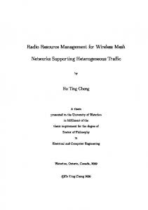
Figure 1 shows the wireless mesh backbone architecture. In this architecture, mesh clients represent other networks such as cellular, IEEE 802.11, IEEE 802.15, and sensor networks. Mesh routers are stationary and they form the backbone of the wireless mesh network. They can be connected to the high speed wireline network via gateways. The gateways, mesh routers and the mesh clients form a three-tier architecture [1], [5], [6]. Mesh clients can form an ad-hoc network that is connected to one or more mesh routers. Mesh routers act as relays to data transmitted between mesh clients or to the wireline network in both directions. Cellular networks, wireless local area networks (WLANs), WiMax networks and other types of access networks can be integrated into the WMN.
Wired Backbone Mesh routers
Gateway
Wireless mesh
Mesh clients Figure 1.1: Wireless Network Architecture 2
1.1.2 Applications
WMNs offer a wide scope of applications including, but not limited to, providing broadband internet access, sharing information on goods and services, gaming, public safety, medical and emergency response, valuable asset security, neighborhood video surveillance, industrial Monitoring. WMNs can also play an important role in disasters reporting and emergency networking.
On the small scale ([7], [8], [9], [10]), such as home or office, wireless mesh networking allows for connections to the internet from anywhere, indoors or outdoors, without wires. Access points are placed in the transmission range of each other to act as packet relays. Technologies such as IEEE 802.11b or IEEE 802.11a are used to provide secure reliable, fast and wireless connectivity. Computers with a wireless card can send and receive data to each other and to the Internet. Small scale WMNs can also be found in coffee shops, hotels, airport lounges and other locations where large crowds gather.
WMNs can cover a metropolitan area to provide broadband access [10], [11], [12], [13], [14], [15], [16]. It provides lower upfront investment cost and less deployment time than the traditional wired network.
3
These applications differ widely in their QoS requirements. A protocol designed to support one set of requirements may not be good for another set. Therefore designing protocols for such networks should consider the diverse requirements, to provide the best performance for each set while achieving fairness among different sets.
1.2 Motivation
As a backbone network, a WMN is required to maintain the same QoS level as its access networks because it is very hard to provide an end-to-end QoS to the users of these networks using a non QoS-aware backbone. In fact, QoS provisioning problem in the mesh backbone resembles to a great extent providing QoS guarantees over the Internet, which is mainly designed for best effort traffic.
In order to provide QoS guarantees over the Internet, two main approaches are used; namely [17], integrated service (IntServ) and differentiated service (DiffServ). IntServ provides QoS guarantees per flow. Therefore, each router in the system should implement IntServ, and every user should make an individual reservation. This implies that each router has to store a large amount of information and heavy signaling traffic may be exchanged throughout the network. As a result, an IntServ-like approach works well with small scale networks or with very high performance (in terms of processing power and memory) routers. DiffServ provides QoS guarantees per flow-class. Only selected routers at the network boundaries implement DiffServ. The remaining routers at the core of the network provide 4
per-hop behavior (PHB). This implies that all complex functions, such as traffic classification and conditioning, are done at the network edges. Core routers are doing the job of routing with a simple DiffServ functionality of per-hop behavior according the class that the packets belong to.
1.3 Objective
The main function of the wireless mesh backbone is to carry the traffic of the access networks and route it to its destination. Our objective in this work is to propose a QoS-aware routing framework for wireless mesh backbones exploiting their unique characteristics. A wireless mesh backbone is different from the Internet architecture in the sense that the wireless links are shared by nature. The links are not isolated; they interfere with each other affecting the quality of transmission and causing packet loss. Also, all the mesh routers are similar in functionalities and capabilities. They can not be divided into core and edge (access) routers. Therefore, it is difficult to apply either the IntServ or the DiffServ QoS models in their current forms proposed originally for the Internet. IntServ requires very powerful routers to handle all the flows’ state information coming from every single user in every mesh client. DiffServ distributes the processing between the core routers and the edge routers, which are the same in the wireless mesh backbone. This implies that DiffServ may need also all the wireless routers to be powerful enough to handle traffic classification, shaping and conditioning. On the other hand, wireless mesh backbones are similar in architecture to wireless ad hoc networks in the sense that they are infrastructure-less 5
networks with shared wireless links. However, the mesh routers are fixed and not batterypowered. Besides, wireless routers carry different traffic pattern from that of ad hoc networks since they interconnect access networks not just mobile users.
In this research, we aim at selecting routes that provide QoS guarantees in terms of delay and signal-to-interference-plus-noise ratio (SINR) to the different traffic aggregates in the wireless mesh backbone. The traffic from the access network is aggregated in the mesh router connected to it based on the service class [5] and then routed to its destination. Each service class has a unique end-to-end delay requirement to be satisfied over the whole route. Each service class also has a minimum SINR to be met at each link of the route.
Our main contribution in this work is a framework for QoS-aware routing in wireless mesh backbone using power control. Our framework is based on a centralized time division multiple access (TDMA) medium access control (MAC) protocol. Our approach for QoS provisioning is to allocate the power of each mesh router optimally in order to discover the routes that maximize the number of simultaneous transmissions in each time slot while meeting both the end-to-end delay and SINR constraints. In general, allocating the resources efficiently for a TDMA-based wireless mesh backbone is a challenging task. It tackles both the QoS routing and scheduling problems taking into consideration the spatial channel reuse. Indeed, power control plays an important role in utilization the bandwidth efficiently. If minimum power is allocated for each hop, this implies that a large number of hops are used 6
in each route. This decreases the delay share of each hop (end-to-end delay is divided among the large number of hops) and hence more time slots (bandwidth) is needed. On the other hand, if maximum power is allocated, the number of hops in every route will be minimal. However, the interference increases, which limits the number of simultaneous transmissions leading to inefficient wireless bandwidth utilization. Therefore, an optimal power allocation is required to realize QoS provisioning with efficient resource allocation.
1.4 Thesis Organization
The remainder of the thesis is organized into five chapters. Chapter 2 gives a summary of literature review. Chapter 3 describes the system model. The problem formulation is presented in Chapter 4. The simulation results and performance comparisons are discussed in Chapter 5. Chapter 6 concludes the research.
7
Chapter 2 Background and Literature Review
Routing and link scheduling are important components in satisfying the QoS requirements and utilizing the network bandwidth efficiently. They have long been addressed in wireless and wireline networks. However, few works have been done for WMNs. Power allocation has also been studied in wireless ad-hoc networks and sensor networks from the perspective of saving power. In the following, we review the literature of routing, link scheduling and power allocation to find the problems addressed and the impact of the proposed solutions in the WMNs. We mention here only the research done on WMNs for the routing and link scheduling. Since the power allocation is not addressed in WMNs we mention some work that was done in traditional ad-hoc networks.
2.1 Routing in WMNs
According to our survey of routing protocols, we classify routing protocols developed for the WMNs according to the QoS level that they provide: Best Effort Routing Protocols or QoS-aware Routing Protocols. Under this classification, we further divide routing protocols according to the number of channels used in data transmission and their combination with the type of antenna, mainly the directional antenna. 8
2.1.1 Best-Effort Routing
Best effort services are those that do not request any QoS guarantees. An example of a best effort application is web browsing in which an internet user requests a web page through a web browser and then waits without any guarantee that the page will not be delayed for a long time, or even though it may not open at all due to network congestion or server overloading. For such type of traffic, the network tries to accommodate as much flows as it can. Therefore increasing network capacity becomes the main concern.
In the wireless environment the main cause for capacity degradation is interference between neighbouring links of the network. In order to increase capacity we should try to alleviate or decrease the effect of interference. Several approaches have been adopted to increase capacity including a better selection of routes, the use of multi-channels, and the use of directional antennas.
Since routing depends on metrics that are mainly measured in the underlying link and physical layers, cross-layer routing has gained much research effort. Routing can be done based on metrics like throughput, delay, packet loss rate, power control, load distribution, and many others that are measured at the link or physical layers. In that case routing protocols are dependent on the underlying structure. So routing protocols can be developed to
9
work on top of a multi-channel architecture while others developed to benefit from using a directional antenna.
Routing protocols design is also highly jointed with the underlying link and physical layers. For example designing a routing protocol for a network using multi-channel MAC protocol will tend to favour channel diversity and load balancing among channels. While routing in networks with directional antennas will try to benefit from the uni-casting capability of the directional antennas and to alleviate problems that aroused for such type of networks. In the next sections, we present and discuss routing protocols developed for besteffort traffic. The protocols are classified based on the number of channels used throughout the network.
2.1.1.1 Routing Protocols for Single-Channel Networks
These protocols focus on choosing a routing metric that selects routes to increase the total network capacity. In [5], De Couto discusses the theory that selecting the minimum hop count as a metric for routing protocols in multi-hop wireless networks tends to achieve poor performance. The reason as declared in the paper is due to the tendency of the routing protocol to include longer links which means distant nodes. The longer the link between two nodes, the more it becomes exposed to fading, noise and other interference. This leads to an increase in packet loss rate and therefore to poor throughput. De Couto introduces a new routing metric, called ETX, which accounts for the link loss rate. A route that has the 10
minimum ETX is selected to be the recommended one. This metric is based on measuring the loss rate of broadcast packets between pairs of neighbouring nodes. A number of small sized packets are sent for the purpose of measuring the link loss rate followed by the reception of replies for these packets. The percentage of successfully received packets out of the transmitted packets indicates the successful transmission rate. The reciprocal of its complementary indicates the estimated number of transmissions required to send a packet on that link.
This metric was adopted by other routing protocols. In [18] it is implemented in two of the well known routing protocols for wireless networks, namely the DSDV [19] and DSR [20] routing protocols. The protocols are implemented in mobile nodes that form an ad-hoc network. A single channel is used and thus if a link is active, all neighbouring links should not be active or there will be interference.
An extension for this work is done by Draves in [21]. Five routing metrics are compared including the traditional hop-count, the proposed link transmission rate in [18], ETX, and another two metrics are the per-hop round trip time (RTT) and the per-hop packet-pair metrics. The per-hop RTT is based on measuring the round trip delay seen by unicast probes between neighbouring nodes. The per-hop packet pair is based on measuring the delay between a pair of back-to-back probe signals to the neighbouring node. According to their results, ETX outperforms the other two metrics when all the nodes are stationary while the 11
traditional minimum hop had the best performance when the sender is mobile. The ETX metric is included in a modified version of DSR which is called Link Quality Source Routing (LQSR) [22].
A simple extension to this work is made by Kulkarni et al in [23]. They modify the previous ETX to suit the multi-rate case. Instead of measuring the number of transmissions using a single rate, they use multiple rates from the set of rates supported by the underlying wireless technology to estimate the transmission time.
2.1.1.2 Routing for Multi-Channel Wireless Networks
In order to increase capacity we should try to alleviate or decrease the effect of interference. Several approaches have been adopted to increase capacity. One active approach is the deployment of multiple channels. Two neighbouring links interfere if they use the same channel. By proper assignment of multiple channels to neighbouring links we can activate more than one link simultaneously on condition that they use different channels. The term “channel” refers to a frequency band, like in FDMA, or an orthogonal code, like in CDMA.
Routing protocols developed for multi-channel wireless networks are often jointed with a channel assignment scheme that enables many neighbouring links to be active simultaneously to increase capacity. Some works are concerned only with channel 12
assignment [24], [25], [26], [27], leaving the routing problem as a standalone problem to be solved on top of the channel assignment.
The work in [24] presents an integer linear programming formulation for the fixed channel assignment problem in multi-radio multi-channel wireless mesh networks. The goal is to maximize the number of simultaneous transmissions in the network. The channel assignment is supposed to be centralized which puts a restriction on the network topology and limits the scalability of the network. In addition, all nodes have to access the channel assignment server, leading to high congestion in the paths to that server.
In [25], Wu et al. proposes a protocol, namely Dynamic channel Assignment (DCA), which utilizes the multi channel capability of the 802.11 physical layer. In this protocol, one channel is dedicated as a control channel for exchanging control messages among all hosts while the other channels are used for data packets. Data channels are assigned dynamically on an on-demand basis. The control channel is assigned to one transceiver while data channels are assigned to the other transceiver(s). By this way a host can listen on the control channel and the data channel simultaneously. The sender uses the control channel to set up connection with the receiver. The request-to-send packet (RTS) includes a list of preferred channels to be used for data transmission. The receiver decides on one of the channels and sends the information to the sender in the clear-to-send packet (CTS). The sender announces the channel used to neighbouring nodes through a reservation packet (RSV). This protocol 13
does not have the multi-channel hidden terminal problem since there will be always one of the transceivers listening to the channel. In addition there is no need for synchronization between the sender and receiver. The disadvantage is the cost of reserving a channel for the small control messages, thus wasting bandwidth.
A similar protocol is proposed in [26] that uses one control channel and N data channels. The difference is that the decision on the channel to use is based on the channel condition at the receiver side. The best channel condition is selected. Although it has a throughput improvement over [25], it still has the same disadvantages.
The protocol in [27] operates with a single radio (transceiver) per host. It does not separate control channel from data channels. The main disadvantage is that it requires clock synchronization among all hosts. Another disadvantage is that it incurs a bandwidth overhead to exchange traffic indication messages. At that time there will be no exchange of data packets.
In [28], Gupta and Kumar show that using one radio per node extensively degrades the capacity of wireless networks. Moreover, the prices of wireless network adapters are decreasing in a way that makes employing more than one network adapter a more cost effective solution. Most of the recent research effort has been directed towards the employment of more than one interface in a mesh router to increase the network capacity. 14
In [29], Draves suggests implementing a routing metric that accounts for the link loss rate to be used in a multiple radio environment. The proposed metric favours the selection of different channels for neighbouring links which will lead to minimizing the interference and thus increasing the capacity. The new protocol was named MR-LQSR (Multi-Radio LinkQuality Source Routing). The new metric WCETT (Weighted Cumulative Expected Transmission Time) allows to trade off channel diversity and path length by adjusting a control parameter. The WCETT combines the link quality in terms of the expected transmission time and the channel diversity by favouring paths that are more channel diverse.
MR-LQSR uses a number of channels which is equal to number of radio interfaces. Thus in the case of two radios, as in their experiment, only two channels are used. Each radio has a fixed channel which has an advantage in that it does not incur a switching delay. On the other side it is a restriction which if relaxed can yield better performance in terms of throughput and which incurs some delay that are tolerable.
In [30], So et al. proposes an on-demand routing protocol for networks with single transceiver nodes benefiting from the multiple channels offered by the 802.11. The protocol, named MCRP, assigns different channels to neighbouring nodes so as to avoid interference. Each node can switch between channels under the constraint that no two neighbouring nodes
15
are switching so that to avoid the deafness problem [31]. The protocol works on a synchronous TDMA access technique which is complex to implement.
In [32] Shacham et al. proposes an architecture for multi-channel wireless networks. Although the architecture is developed for network with single radio nodes, it can be extended to multi-radio nodes network. The main restriction in this architecture is the tight coordination it requires among nodes which cannot be easily guaranteed.
An attempt to assign channels to interfaces and schedule flows is made by Bahl in [74]. Bahl proposes a link layer solution named Slotted-Seeded Channel Hopping (SSCH). This work is implemented in networks with single interface nodes but can be extended to multiple interface nodes. In SSCH, nodes hop between channels after fixed intervals based on a schedule. This schedule is published to neighbouring nodes so that two nodes can communicate by adjusting their schedule to have a common channel at some time. The paper includes also a flow scheduling algorithm per each node. Bahl did not discuss a routing protocol to be implemented on top of his work.
A joint channel assignment and routing protocol is proposed in [34], [35]. This work by Raniwala et al. focuses on improving the capacity of wireless mesh networks that is used as an intermediary between the wired backbone and the mobile mesh clients. Thus all the traffic is directed towards specific gateway nodes. They assume each node to have more than one 16
radio and each radio can switch among the available channels. Two channel assignment and bandwidth allocation techniques are proposed. The first is based on network topology and the other is based on traffic load. They claim that any routing algorithm can work efficiently on their channel assignment techniques. However they implement a routing protocol that has its routing metric as the shortest path and another one with randomized multi-path routing.
In [33], Pradeep proposes a joint channel assignment and routing protocol. This work allows for a free traffic load from any point in the network to the other. He considers switching latency in the work and tries to minimize it by decreasing the channel switching rate for one interface. He also proposes a new routing metric incorporated into an on-demand routing protocol. The proposed Multi-Channel Routing (MCR) metric combines the measured link expected transmission time (ETT) and switching costs into a single path cost.
2.1.1.3 Routing for nodes with Directional Antenna
Another approach for improving wireless network capacity is the use of directional antennas [36], [37], [38], [39], [40]. By beam-forming at the transmitter we can restrict the transmission area, reducing interference and alleviating the exposed terminal problem. Therefore capacity can be greatly improved and we can achieve higher throughputs. Placing the directional antenna at the receiver side can reduce the hidden terminal problem by only listening to the expected area of transmission.
17
Directional antennas have also an impact on the network layer. They help in finding routes with less hop count [38] due to the longer transmission range of directional antenna. They can also help in finding energy efficient routes [39] and interference-aware [40] routes.
On the other side, using directional antennas has founded new problems including new kinds of hidden terminal problems and deafness [41] and capture [36]. Another problem that arises is the discovery of the neighbours [42]. These new category of problems imposes a tradeoff between gaining benefits of using directional antennas and solving or adapting to the problems.
2.1.2 QoS-aware Routing
With the recent advances in communication technology and the flooding of multimedia services through the internet, QoS consideration in networking is becoming imperative. Providing QoS is a challenge to networking services’ providers especially in the wireless environment. Different layers can share in fulfilling QoS requirements individually or integrated with others.
Services guarantees are a typical requirement for applications involving audio and video transmission such as Voice over IP (VOIP), distant learning using online multimedia 18
transmission and video conferencing. This type of traffic is characterized by having variable bit rate (VBR). Allocating bandwidth is a challenge in that case since if it is allocated according to the maximum rate then resources are wasted and other applications will be blocked while there is unused capacity. In addition, calculating the effective bandwidth in the wirelesss environment is not a trivial task.
Several metrics are used to specify QoS requirements in networks such as minimum required throughput or capacity, maximum tolerable delay, maximum tolerable delay jitter, and maximum tolerable packet loss ratio. An application may request guarantees on one or more metrics for its QoS. In the next sections, we present and discuss the different routing protocols developed to satisfy QoS requirements for traffic flows.
2.1.2.1 General Routing Protocols
A route is scanned for QoS satisfaction in a procedure similar to route discovery in conventional routing protocols. The source node sends a route request packet with the QoS guarantees required on the route such as minimum required bandwidth, total delay bound, packet loss rate (PLR) to the destination. This can be done either by broadcasting (flooding the network) or using a previously discovered route or a list of routes. Every node receiving the route request packet carrying the required QoS guarantees compares its own measured metrics with the required metrics bound found in the packet header. If not satisfying the
19
requirements, a node failure packet is sent back to the source node to start a new route discovery or to an intermediate node to perform a route repair procedure.
In [43], a source node initially selects a neighbour that is closest to the destination according to location information service provided in the network. On the way from source to destination every node compares its PLR with the maximum PLR in the packet header and the accumulated PLR so far. If the PLR constraint is violated a route failure is sent back to the source to start a new QoS route discovery. Once the route request packet reaches the destination, the available bandwidth required on each intermediate node is calculated and an admission request message is sent to the source. If the bandwidth requirements are satisfied then the bandwidth is reserved in that node and this information is broadcasted to neighbouring nodes. If the bandwidth requirements are not satisfied an admission refused message is sent to the next node on the route to the source to start a route repair procedure. The route repair is a partial route discovery from the node received the route repair message to the destination.
In [44], three versions of a routing protocol schemes are introduced. The protocols are designed assuming that data flows are established between client nodes and the gateway. Two client nodes will always communicate through their parent gateway. Therefore every node needs to know a route to the nearest gateway only. The protocol scheme is named mesh routing protocol (MRP). The first version of the protocol is MRP On-Demand (MRP-OD). A 20
new node joining the network broadcasts locally (one hop) a route discovery (RDIS) message. All the nodes receiving the RDIS message will reply with a route advertisement (RADV) message with the metrics of their routes to the nearest gateway. The protocol is benefiting from the fact that all connected nodes already know routes to gateways and the significant routing metrics of those routes. If the joining node did not receive an RADV message it will keep sending RDIS messages. Upon reception of RADV messages the node will selects one or more routes according to its QoS requirements. By this way, the setup of the upstream route from the node to the gateway is completed. The return path does not have to be the reverse. Thus a return path discovery is established by sending a registration request RREG from the node to the gateway. When the gateway receives the RREG message it replies by registration acknowledgment (RACK) message. Loss of any of the RREG or RACK requires re-initiation of the discovery process. Upon reception of the RACK the joining node starts sending and receiving from the internet.
If a link loss is suspected, during the transmission and reception of data packets, the node enters a verify-link state. In the verify-link state, the node keeps sending route check (RCHK) packets unicasted to next hop. If a reply is received then the route is working again, otherwise the node switches to a disconnected state. If a node losses its route to the gateway, all its children will lose their route also. Hence when a node losses its connection with the gateway, it sends a route error (RERR) message to all its children. When losing the connection to a gateway, a node, and therefore all its children, will reinitiate a route discovery process. 21
The second version of MRP is MRB beacon mode (MRP B). Instead of sending RDIS messages to neighbours to discover a route to a gateway, a node listens to periodic beacons sent by nodes in the network to advertise routes. After collecting beacons from neighbours, the route selection and registration proceeds as in MRP-OD. A link loss is determined by missing a predefined number of beacons. This version reduces the delay of route-break detection but increases routing overhead.
The third version is the MRP hybrid (MRB H) which is a combination of the previous two versions. A new node joining the network or returning from a disconnection state sends RDIS messages to discover routes to gateway instead of waiting for the beacons. While a link loss is detected by not receiving a predefined number of beacons. This version has faster route discovery and link failure detection. However, it imposes more routing overhead than the previous two versions.
2.1.2.2 Location-based Routing
For non-position based routing protocols, a routing protocol has to flood the network with route request packets to discover the route to destination. This overhead can be greatly reduced if the node has information about the destination location. In position based routing protocols [45], the source node sends a packet with the destination position contained in its 22
header to the closest neighbours to the destination. The neighbours forward the packet to the next closest neighbours to the destination and so on till the packet reaches the destination. The destination can be a single node or a group of nodes in a certain geographic area which is called geocasting [46]. Location information can be gathered using GPS or other position determination devices [47]. A recent protocol [43] used ultra wideband (UWB) technologies to estimate position. In [43], the source node sends a route request packet to discover a route that satisfies the QoS requirements. The packet is sent in the estimated direction to destination as long as the QoS requirements are satisfied. If the QoS requirements are violated a route failure packet is sent to the source node to begin another QoS route discovery.
2.1.2.3 Routing in Differentiated Service Networks
In [49], an architecture for Differentiated services provision in the wireless mesh backbone is discussed. Hai et al. proposes a QoS routing and MAC scheme for WMN backbone routers. They recommend the routing to be class-based. For each traffic class the routing protocol should select routes that satisfy the QoS requirements of that class. They suggest using an ondemand routing protocol similar to AODV to reduce signalling overhead and they assume the network to work with a single channel. This work is preliminary and is an open issue for further research.
23
Another approach to provide QoS routing is addressed in [48]. The authors divide the network into clusters and suggested the routing to be done on two levels: inter-cluster routing and intra-cluster routing. Inter-cluster routing aims to route data cluster by cluster. While the intra-cluster routing aims to route data inside the cluster. This coarse granularity routing can prove to be efficient in terms of scalability but is worse in terms of interference and thus throughput and delay.
2.1.2.4 Multiple-Constraints Routing
Traffic flows vary in their requirements. Flows can be bandwidth-sensitive requesting a minimum bandwidth or delay-sensitive requesting a maximum delay bound. Others can request for maximum packet loss rate (PLR) bound. Flows requesting multiple QoS metrics guarantees impose more difficulty. Solving a multi-constrained path problem is a NPcomplete [49] in many cases such as when the metrics are additive [50]. Even satisfying one constraint may become NP-complete when link interference is taken into consideration [51], [52].
Solving the multi-constrained routing problem in WMNs is addressed in [53]. The authors propose a routing scheme based on Mean Field Network (MFN_RS). The goal is to find a solution for the routing optimization problem using a computational method that is faster than the Simulated Annealing (SA) approach.
24
The protocol in [43] uses heuristic algorithms to solve the problem. The researchers divide the two-constraint problem into two one-constraint problems. A QoS route discovery is done on two steps. The first is to discover a route that satisfies the packet loss rate (PLR) requirement. The second step is to check if the discovered route satisfies the other requirement which is either bandwidth or delay.
2.1.2.5 Multi-Channel Routing
Multiple channels are presented as a solution for the interference problem. Channels can be orthogonal codes (CDMA) or frequency bands (FDMA). A routing protocol that is built on a multi-channel network is mostly jointed with the channel assignment problem. Channel assignment was investigated in several works [24], [25], [26], [27]. A centralized channel assignment performs better than a distributed one. However it can be a bottleneck in the network.
A Bandwidth Aware Routing (BAR) protocol is presented in [54] following an interference aware channel assignment. The routing protocol guarantees bandwidth for each flow assuming the bandwidth for each link is known. It is assumed that each node is equipped with two network interface cards (NICs). Each NIC is tuned to a different channel. Different nodes use different channels with the constraint that two neighbouring nodes must 25
have a common channel to communicate. The channel assignment is centralized and static which means that it will last as long as there are no new nodes added to the network.
2.1.2.6 Multi-Path Routing
Multipath routing is used to maximize utilization of network resources. With multipath routing, a node chooses several links (or routes in case of vitual circuit (VC)) for the same destination. If properly managed, it can aggregate resources of multiple paths, increase admission rate, increase throughput and improve reliability.
The design of a multipath protocol requires much care about routing overhead and coordination among neighbouring flows. The protocol proposed in [55] limits the number of multiple paths to a number specified by the flow. The protocol, named multi-path dynamic source routing protocol (MP-DSR), is based on the existing Dynamic Source Routing
protocol (DSR) and takes advantage of its distributed on-demand nature. It seeks to compute a set of unicast disjoint routes that can satisfy a minimum end-to-end reliability requirement. The path reliability is calculated based on the link availabilities of all links along a path. Link availability is defined as the probability that a link is available for a defined period of time. The calculation of link availability is based on the node’s movement; a constraint which is not found in WMNs.
26
The same approach of path limiting is addressed in [56]. Chen et al. proposes a ticket based multipath routing. The source node issues probes to discover routes. Each probe is
assigned a number of tickets that is equal to the number of required multiple paths. The number of tickets is related to the stringency of the constraint requirements.
2.2 Power Allocation
As the wireless routers in the WMN are not battery-powered, power allocation becomes an important factor in designing a routing protocol. It provides an additional degree of freedom beside the traditional frequency, time and code degrees. Power allocation has been investigated in different research works related to routing problems in WMNs. We classify these protocols into those that concern about saving power and others that use the available power constrained only by the maximum limit.
2.2.1 Power Saving Techniques
Many proposals have been developed that aim at saving power [57], [58], [59]. Reducing both energy and interference is the target of the work done in [57]. The authors discusses the topology control techniques developed in the literature of ad-hoc and sensor networks. They prove that topology control though reduces energy but is not enough to reduce interference. They propose an interference-minimum construction that preserves connectivity of the nodes and provide paths that are longer by a constant factor than the shortest paths in the original 27
network. In [60], the authors assume a conflict free medium access on which they implement their energy-efficient QoS topology control. They accommodate traffic flows according to the capacity available after applying their energy saving algorithm. All these works concern about saving energy which limit the QoS satisfaction for the flows in the network. This is acceptable in a network with battery-powered nodes such as in ad-hoc or sensor networks. However, in WMNs the concern is directed towards increasing the network capacity while satisfying the QoS requirements.
2.2.2 Using Available Power
An early work for adjusting transmission power in wireless networks is presented in [61]. The work provides an analytical model to adjust the transmission power for slotted ALOHA packet radio networks for the sake of reducing interference. Three different methods for allocating the power are studied in [61]. The first one is the shortest-hop allocation, which implies the power is allocated just to reach the closest neighbor (shortest hop). The second method allocates the power to reach the longest hop within the transmission range and the third uses the maximum power. It has been shown that the second method causes the smallest interference compared to the other two. The advantage of these methods is their simplicity. Little computation is required to decide for the next node to receive the packets. The disadvantage can be seen in ignoring the traffic load in computing the relay node. In the three strategies, traffic load is not taken into consideration. In addition, the decision is either the farthest or the nearest, neglecting the 28
chance of having better decision for an intermediate relay node. This work is done for best effort traffic.
In [62], maximum power allocation is used in order to achieve opportunistic routing. Using a high transmission power enables transmitting to far nodes in one hop. All the nodes (routers) in the transmission range of the transmitting node receive a copy of the transmitted packet. Some may not receive the packet successfully due to wireless channel impairments such as fading and interference. Therefore, the receiver nodes agree on one of them to be the next node in the path and forward a received packet in a similar way till reaching the destination. This work mainly addresses the link quality problem without any QoS considerations.
Wei et al. [63] introduces an interference-aware routing algorithm and a centralized TDMA scheduling scheme. The work in [63] aims at achieving high channel utilization by minimizing the interference. However, it does not address QoS issues in the route construction or in the scheduling scheme. Tao et al. [64] proposes an algorithm for centralized scheduling and routing using concurrent transmissions. However, the algorithm is based on routing trees where the route of the tree is the centralized controller. This implies that some mesh routers can communicate only to reach others via the controller, which indicates a potential single point of failure in the network. In addition, the paper does not address the QoS issues. 29
2.3 Summary
In this chapter, we present and discuss the routing protocols developed for the WMNs and the power allocation techniques related to our work. The work done focuses on increasing the network capacity which is achieved by avoiding or reducing interference. Approaches to reduce interference include using multiple channels, directional antennas or properly managing the media in the case of a single channel by introducing new metrics. Most work done addresses the best-effort traffic. Satisfying QoS requirements for the traffic increases the complexity of the problem.
It has been shown that despite the diversity and richness of work done, the existing work does not fully address the unique characteristics of WMNs, mainly: transmission power availability (up to maximum power) and stationary property of the wireless routers. We aim to make use of these characteristics to support QoS routing in WMNs.
30
Chapter 3 System Model
The network under consideration consists of 25 routers connected to each other through wireless links. The routers are distributed in a grid topology on an area of 1500 m2. The location of sources and destinations are randomly chosen. Each node (router) knows its location and can adjust its transmission power to any value between zero and its maximum power level Pmax. We assume line-of-sight (LOS) transmission is available in all backbone links and also in all access links (between mesh routers and mesh clients). All the backbone wireless router transceivers are assumed to work in a half-duplex manner; they cannot send and receive at the same time.
3.1 Path Loss Model
Since all the backbone and the access links are static, it is reasonable to assume a free space path loss model. At any distance d from the transmitter, the path loss PL(d) at a particular location is random and distributed log-normally (normal in decibel units, dB) about the mean distance-dependent value [65]. That is ___ ___ ⎛d ⎞ PL (d )[dB ] = PL (d ) + X σ = PL (d 0 ) + 10n log⎜⎜ ⎟⎟ + X σ ⎝ d0 ⎠
31
___
where PL (d ) is the path loss due to distance, X σ is a zero-mean Gaussian distributed random variable (in dB) with standard deviation σ (also in dB), d0 is a close-in reference distance (close to the transmitter) and n is the path loss exponent which indicates the rate at which the path loss increases with distance. The distance-dependent path loss can be calculated using the formula ___ ⎛ G G λ2 ⎞ PL (d ) = −10 log⎜⎜ t r 2 2 ⎟⎟ λ = c f ⎝ L(4π ) d ⎠ ,
where Gt and Gr are the transmitter gain and receiver gain respectively, L is the system hardware losses, c is the speed of light, f is the carrier frequency. The signal power received at the receiver, Pr, can then be calculated using the formula
Pr (d )[dBm] = Pt [dBm] − PL (d )[dBm]
where Pt is the signal power at the transmitter (in decibel milliwatt, dBm) and d is the distance between transmitter and receiver. In order to define a path loss for a link, we will use a slightly different notation which is the path gain G. We will define path gain for each pair of transmitter-receiver. Therefore, for a transmitter T(l) of link l and a receiver R(l) of link l, we have a path gain G(T(l),R(l)). With this notation, we can define the signal-to-noise-plus-interference ratio for a link l to be
SINR(l ) =
G (T (l ), R(l )) P(T (l )) ∑k∈L,k ≠l G(T (k ), R(l ))P(T (k )) + N 0
32
where N0 is the thermal noise power at the receiver which is normally considered to be constant, and G(T(k),R(l)) is the path gain between the transmitter of link k and receiver of link l.
3.2 Traffic Model
Since a wireless mesh backbone connects different networks such as cellular, IEEE 802.11, IEEE 802.15 and sensor networks, it is expected to have traffic with different characteristics and different QoS requirements. Each router has traffic flows aggregated from different sources and going to different destinations. The packet traffic often follows an on-off behaviour. During the on period a burst of packets is generated. The distribution of on and off periods is the burst level description of the traffic. For example voice-packets’ modelling assumes on and off periods to be exponentially distributed.
Packet level description of the traffic, such as packet arrival and packet size, is of more complexity due to the many factors affecting it including different applications, users’ profiles and network protocols. Traditional modeling assumes a Poisson process or periodical arrival for the packets. However, it is found in [66] that these models are not accurate for aggregate traffic. It is found in [67], through real measurement and statistical analysis of traffic data gathered from wide area network (WAN) and Ethernet, that the aggregate packet arrivals from multiple sources can be well modelled by self-similar processes with long range dependence and heavy-tailed distribution. A self-similar model for traffic means that a
33
segment of the traffic at sometime scale looks or behaves just like an appropriately scaled version of the traffic measured over a different time scale.
Several processes can be used to generate the self-similar traffic. In [66], an M/G/∞ queue model is suggested for generating self-similar traffic. In [68], it is proved that self-similar traffic can be generated by superposition of multiple i.i.d. on-off sources which have a heavy tailed distribution with infinite variance for the on and off periods. The work done in [69] proves through real measurement and statistical analysis that self-similar nature is found to exist in cellular networks with mobile nodes. In [70], the author proves that using a Markov Modulated Poisson Process (MMPP) for modelling the traffic accurately approximates the characteristics of Internet traffic.
No work so far, until this thesis was written, had been done to model the aggregate traffic in wireless mesh networks. We will assume that the traffic follows an MMPP model with ON and OFF periods following an exponential distribution. The probability to switch from the ON to the OFF period is α, and that from the OFF to the ON is β. Packets arrival during the ON period is a poisson process with arrival rate λ. The arrival rate varies for each traffic flow and for different experiments.
The following figure shows the 2-state Markov model used for packet arrival. During the ON period, a series of packets are generated. In the OFF period, no packets are generated. 34
Duration of each ON and OFF period is estimated by independent exponential laws of parameters α and β. The mean duration of the ON period (Ton) and the OFF period (Toff) periods are Ton =
1
α
and Toff =
1
β α on
off
β
Figure 3.1: The on-off traffic Model
The activity factor for the packets’ source can be calculated as Activity factor =
Ton β = Ton + Toff α + β
We consider two different classes of service with different end-to-end delay bound requirements Dr(1) and Dr(2). The two classes also have different SINR requirements,
SINR(1) and SINR(2) respectively, at each link so their data can be decoded correctly (with sufficient bit error rate) at each forwarding hop. We assume that the data will be decoded at each forwarding hop and then re-sent so the bit error rate will not be accumulated over the whole route causing severe degradation in the SINR at the final destination.
35
3.3 Medium access
We consider a centralized control TDMA MAC protocol. The control is done by one of the wireless routers with special capabilities. The exchange of control information is done by direct communication between the routers and the controller for specific or common control messages. However, for data transmission, all the routers communicate directly with each other in an peer-to-peer manner.
In the TDMA-based MAC, time is partitioned to fixed length frames. The frame structure contains a beacon period (control sub-frame) in addition to the contention-free period (data sub-frame), which is partitioned to time slots with equal duration. The controller allocates the time slots and the power for each wireless router via signaling messages broadcast on the beacon period. We assume the controller is aware of its location and the location of each wireless router.
The time frame structure is shown in figure 2 where the frame is divided into two subframes: a control sub-frame and a data sub-frame. The control sub-frame is where the communication control part takes place. This includes synchronization of slots and frames, clustering, routing messages, power measurement, VC setup, ACKs, etc.
36
frame 1 2
N
Control sub-
Data
frame
sub-frame
Figure 3.2: Time frame structure
At the end of the control sub-frame, each node has learned the data slots assigned to it. In order to support real-time traffic, data slots must be reserved prior to the data sub-frame. The number of data slots is determined according to the bandwidth requirement of the traffic flows.
3.4 Effective Bandwidth and Admission Control
An important approach that is considered in the admission control for multiplexing variable bit rate (VBR) traffic is the effective bandwidth. It captures the statistical multiplexing gain achieved from aggregating a large number of bursty sources. Given the traffic characteristics of each source and its QoS requirements, we can obtain the relation between the required capacity, C L , and the number of sources to be admitted, N s . The effective bandwidth
37
BE =
CL ranges between the peak rate and the average rate to achieve a balance between Ns
QoS assurance and high utilization. We use simulation to find the effective bandwidth that achieves the acceptable packet loss rate for all the traffic flows.
3.5 Summary
In this chapter, we propose a network model to provide QoS for VBR traffic. The network is assumed to be clustered. Each cluster is managed by the cluster head. A deterministic TDMA is used to take advantage of the interference-free medium. A transmitted signal is subject to free-space path loss which is a function of the distance the signal travels. Packet arrivals follow an MMPP model in which there are 2 states: ON and OFF state. During the ON state, inter-arrival times between packets follow an exponential distribution.
38
Chapter 4 Problem Formulation
In this chapter, we present our formulation for the joint routing and link scheduling problem. We first define some variables that will be used in the formulation. Then the problem is formulated as an optimization problem.
4.1 Variable Definition
The variables used in the formulation are as follows: (i)
A route r ∈ R, where R is the set of all routes in the network, consists of Lr links. Any two subsequent links cannot be active at the same time because each node has only one transceiver.
(ii)
Each route r has a maximum end-to-end delay requirement Dr. to each of its packets. The end-to-end delay of a packet is the time it takes to travel from the source node to the destination node including intermediate links’ transmission delays and nodes’ queuing delays. Each link transmission delay equals the reciprocal of the link bandwidth (data transmission rate) which is constant. For the estimation of queuing delay, we use the average queuing delay at each node. Because we have fixed packet size and frame size, the M/D/1 can be used to 39
model the queues in our network [1]. Therefore the average waiting time for a packet in a queue, dq can be calculated as
d q (λ ) =
t s (1 − λt s / 2) 1 − λt s
where ts is the service time, and λ is the arrival rate. (iii)
A(l,s) is a binary variable which is equal to 1 if link l is active in time slot s; otherwise, it is 0.
(iv)
A set L of wireless links connects the nodes of the network. A link l ∈ L can be represented by its two nodes l = (T(l), R(l)),where T(l) is the transmitter node, and R(l) is the receiver node. The transmitter node T(l) uses a power P(T(l)) to transmit on link l. The path gain for link l is given by G(T(l),R(l)), and models the transmitter and the receiver amplification gains, as well as the attenuation of the signal due to distance, fading and shadowing.
(v)
Pmin is the minimum power required to transmit a signal on a link given the link distance and the sensibility of the receiver. Pmax is the maximum transmission power.
40
4.2 Problem Formulation
The problem is divided into two parts; the first part is obtaining all combinations of all the possible routes for all source-destination pairs; the second part is to solve the link scheduling problem for each combination of routes which is then used to find the best combination. The first part is very time consuming and requires a heuristic to reduce its large time complexity. The second part is formulated by an optimization problem and can be solved in a reasonable time (hundreds of milliseconds to few seconds) on current computers’ configuration. We start our problem formulation by presenting the optimization problem to solve for the link scheduling. After that, we discuss the heuristic we used to reduce the time complexity of finding the best combination of routes.
The link scheduling problem can be formulated as:
∑∑ A(l , s)
(6)
+ d q ) ≤ Dr ; ∀r ∈ R
(7)
1 S .t s
maximize
L
S
l =1 s =1
subject to
∑ (t
l∈Lr
s
SINR (l , s ) =
G (T (l ), R(l )) A(l , s ) P(T (l )) ≥ hr ∑k∈L,k ≠l G(T (k ), R(l ))A(k , s) P(T (k )) + N 0
where hr is the SINR threshold for route r, and N0 is the white noise power 41
(8)
A(l , s ) Pmin ≤ P(l , s ) ≤ A(l , s ) Pmax ; ∀l ∈ L
∑
{i , j }∈L
A({i, j}, s ) +
∑ A({ j, k}, s) ≤ 1
(9) (10)
{ j , k }∈L
∑ A({i, j}, s) ≥ 1
(11)
{i , j }∈L
A(l , s ) ∈{0,1}; ∀l ∈ L
(12)
The objective function is the maximization of the average network throughput, where S is the number of slots in one frame, L is the set of all links in the network, and ts is the duration of one time slot. Constraint (7) is the delay constraint. Each link delay is the summation of transmission and queuing delays. The constraint ensures that the summation of delays over all the links of one route (flow) during the slots allocated to that route does not exceed the delay bound. Constraint (8) ensures that the signal to interference noise ratio (SINR) is greater than the required threshold. Constraint (9) is the upper and lower bound for the link power. Constraint (10) ensures that no two links having a common node can be active at the same time slot. Constraint (11) states that at least there should be one link active given that the packet queue is not empty.
42
4.3 Reducing problem complexity
The problem is a mixed integer non-linear programming (MINLP) problem which is difficult to solve and takes too long time for a large number of links in the network; therefore, in order to reduce the time to solve the problem, we take two consecutive steps: the first step is to remove the non-linearity of the problem; and the second is to find a heuristic to reduce the search time in the solution set.
4.3.1 First step: linearization
Looking into the problem formulation, we can find that SINR constraint is the only one that introduces non-linearity; this is due to the presence of the product of the two variables, the link binary variable and the link power variable. A common way to eliminate the nonlinearity of this kind is to use the big-M method [3]. The SINR constraint should be verified if the link explored is active, otherwise it should be redundant. This can be formulated as follows:
G (T (l ), R(l )) P(T (l )) ≥ h(∑k∈L ,k ≠l G (T (k ), R(l ))P(T (k )) + N 0 ) − M (1 − A(l , s )) where M is a big positive number; if the link l is active at slot s, then A(l,s)=1 and the second term in the right hand side is of zero value; however, if link l is not active, then A(l,s)=0 and the second term of the right hand side is of a very large value that the formula will be verified
43
in all cases. Since variables are not multiplied by each other, the formula is linear and hence of lower complexity than the original one.
4.3.2 Second step: Finding a heuristic
A heuristic is a technique used to solve a problem with a high computational complexity in a reasonable time but without guaranteeing to achieve the best solution. One of the widespread techniques is the genetic algorithm.
A Genetic Algorithm (GA) is a search technique. It is mainly used as a heuristic to find sub-optimal solutions from within a large set of possible solutions in a reasonable time. A GA involves operations that help evolve towards better solutions. It starts by selecting an initial population of chromosomes representing a subset of the large set of all possible solutions. Each of the population chromosomes is evaluated using a fitness function that is defined according to the problem. Some of the chromosomes are selected from the population to undergo a crossover operation. This operation results in new chromosomes that inherit the characteristics of its parents. A mutation operation may occur according to some probability which alters one of the chromosomes to yield a slightly different new chromosome. These operations are repeated for several generations till we are satisfied about the fitness of the last generation. The chromosome with the highest fitness value in the last generation is the best solution obtained from the algorithm.
44
4.4 Mapping to our routing problem
Our problem is to find the best set of routes for all source-destination pairs that maximize the network throughput. Each chromosome represents a set of possible source-destination routes, one route for each source-destination. A gene in the chromosome represents a node ID; therefore, the chromosome is a chain of node IDs that constitute the different routes of the network. A set of possible solutions are chosen randomly from the set of all possible solutions to produce the initial population. Operations that are done on the population are selection, crossover, and mutation. The generation is then evaluated and the process is repeated.
4.4.1 Selection
Two chromosomes are selected using the roulette-wheel selection to undergo a crossover operation. The roulette-wheel selection selects chromosomes in proportion to their fitness value; the more the fitness value, the more the chance to be selected. In order to achieve that, all the population chromosomes are evaluated using the fitness function. The probability of selecting chromosome i with fitness value fi is thus
pi =
fi Np
∑f j −1
where Np is the population size. 45
i
4.4.2 Reproduction (Crossover)
Each two selected chromosomes are then combined to generate two new chromosomes. A part of one chromosome that is selected randomly is replaced by another random part from the other chromosome and the same for the other chromosome. The new chromosomes are validated so that they do not evolve to an unfeasible solution. Then they are evaluated and join the population only if they have a fitness value that is higher than then the smallest fitness value of the population. By doing that, we guarantee that the crossover operation does not worse the population fitness; either improves or leaves it as it is. The two new chromosomes, then, replace the least-fitness chromosomes in the population so that the population size remains constant.
4.4.3 Mutation
Mutation is the process of altering a gene (a node ID) so that it becomes any other valid gene (another node ID). This operation helps in introducing new solutions that may not be reached through crossover operations. We perform mutation with a probability of 0.1; a typical value as mentioned in [75]. The gene is selected randomly (uniform random) from all the genes in the chromosomes other than the first and last gene of each route (source and destination).
46
Solution steps
We assume our network to be a cluster within a clustered network. The optimization problem is to be solved in the cluster head which acts as a controller for its cluster. The results are sent to the cluster members to act upon. The cluster controller collects the required information (QoS requirements(delay, SINR), traffic rate) from its cluster members and from other clusters through communication with the other cluster controllers.
The following procedure describes our framework: 1. The controller polls the other routers in its cluster and the other cluster controllers via signaling messages to get the location information and QoS parameters. The location information is acquired for new members only since the network members are static. The current source routers aggregate the traffic from the mesh clients connected to them based on the class of service required. Then, they respond to the network controller by appropriate signaling message with the required information.
2. Based on the location information of the routers and the maximum power Pmax, the controller obtains all the possible routes for each source router according to the distance between this router and the other routers.
3. The controller tries the possible combinations of the different routes of all the source routers. It tries to find the links slot scheduling (which links can be active at each slot) and also the combination of routes that satisfies the QoS requirements and maximizes the network throughput. At each combination and for every time slot, all the links that can operate simultaneously are selected taking into consideration that consecutive links from the route 47
cannot work simultaneously in the same time slot. The links that can share a certain time slot are selected based on the SINR value at each receiver of these links.
4. The different combinations are compared and the combination that maximizes the network throughput is selected by the controller.
5. The routes information together with the links’ schedule is sent to the nodes participating in the process to begin transmitting at the next data slot.
6. In order to admit any new mesh client, the controller goes again to Step 3 until no other flows from any service class can be admitted, which implies that the maximum possible number of flows is reached. Figure 4.1 is a flow chart that summarizes the previous steps.
48
Start
Control phase of a new frame: Collect traffic information (rate, max power, QoS req.)
Find all possible routes for each sourcedestination pair
Try different combinations of the routes to find the best one among them (Use genetic algorithm to reduce search space). This step includes finding the optimal link schedule
Disseminate the routes with the link schedule to the nodes to transmit during the data phase
Data phase: Data transmission occurs
Figure 4.1: Flow chart of solution procedure
49
Chapter 5 Simulation and Results
In our simulations, we consider a network cluster of 25 static nodes in a 1500x1500 m2 area. We assume the carrier frequency to be 2.4 GHz. Speed of light is 3x10⁶m/s. The transmitter and receiver amplification gains are 100 each; therefore, a link of distance d has a link gain (path loss) of 2
⎛ ⎞ 1 3x10⁸ ⎟ 2 G = 100 x100 x⎜⎜ 9 ⎟ ⎝ 4 x3.14 x 2.4 x10 ⎠ d
The ambient thermal noise at each node N0 = 10-12 W. The minimum SINR threshold h=10. The maximum transmission power Pmax = 300 mW. Simulation run-time is 100,000 time slots. Receiver sensibility is -120 dB. The delay requirement of each route, Dr, is a random integer.
We compute optimal solutions by simulating the network in Matlab and solving the optimization problem using lpsolve [2].
50
5.1 Experiment 1
In this experiment, we consider the 25 nodes to be randomly distributed over an area of 1500m2. We randomly set 12 source-destination pairs in the network. Traffic sources are modulated as a Markov-modulated Poisson Process (MMPP) with ON and OFF states. Transition probabilities are 0.1 from the ON to OFF state and 0.9 from the OFF to the ON state. During the ON state, packet arrivals are modeled by a Poisson process. The Twelve traffic flows vary in their average arrival rate and bandwidth requirement. Several runs are performed to find the average packet losses. Packet losses occur due to the buffer overflow and packets’ delay expiration. Packet queue at each node can store up to 50 packets. Simulation time is 100,000 time slots. Delay deadlines are set to be equal to double the average inter-arrival time, i.e. a packet can wait for only 2 packets’ average arrival. Results are represented as per the traffic load. Traffic load is defined to be the ratio of total average bandwidth of all traffic to the network bandwidth, or in mathematical notation F
Load =
∑B f =1
f
C
where Bf is the estimated average bandwidth for flow f, F is the set of all flows, and C is the network bandwidth.
51
45 40 35
% Pkt loss
30 25 20 15 10 5 0 0.357 0.385 0.417 0.455 0.5
0.556 0.625 0.714 0.833
1
1.25 1.471 1.667
2.5
Traffic load
Figure 5.1: Percentage of packet Loss vs traffic load
It can be seen from the figure that packet losses exist in all traffic load values even in the light traffic loads; this can be justified by the fluctuation of the packet arrival around its average arrival times.
In the figure, it is shown that at a unity traffic load, i.e. the network bandwidth is equal to the total average bandwidth of all flows, the flows experiences a packet loss of about 8.5%. It is up to the flows’ sources to specify the acceptable loss rate. If the loss rate required is less than 8.5% (assuming all flows have the same packet loss requirement) then we should go
52
further left in the traffic load access, which means the effective bandwidth is going towards the peak rate of the flows.
5.2 Experiment 2: Frequency Reuse
In this experiment, we run several runs with different number of flows (source-destination pairs). In each run, we calculate the number of active links working in one frame. We define the frequency re-use index to be the number of active links in one frame divided by the number of slots in one frame. The simulation results are shown in figure 5.2.
It can be noticed that the trend of the frequency reuse index is to increase by increasing the number of running flows in the network. This can be justified by the tendency of the flows to have shorter hops which is illustrated in figure 5.3. When the number of flows increases in the network, and hence the number of links, over the same network area, it becomes difficult to run more links simultaneously; thus, frequency re-use is seen to stabilize at the higher number of flows.
53
1.6 1.4 1.2
links/slot
1 0.8 0.6 0.4 0.2 0 2
3
4
5
6
7
8
9
10
11
12
10
11
12
Number of flows
Figure 5.2: Frequency re-use index 6
Number of hops/route
5
4
3
2
1
0 2
3
4
5
6
7
8
9
Number of flows
Figure 5.3: Average number of hops per route 54
It is observed that by increasing the flows in the network, flows tend to have more links. This is due to the tendency to have shorter hops in crowded networks.
5.3 Experiment 3: Maximum throughput versus Minimum power
In this experiment, we compare the results of the maximum-throughput algorithm to that of a power-saving algorithm in terms of packet loss. Both algorithms satisfy the QoS requirements. Results are shown in figures 5.4 and 5.5.
50 45 40
% pkt loss
35 30 25 20 15 10
minimum power maximum throughput
5 0 0.541 0.575 0.613 0.657 0.708 0.767 0.836 0.92
1
1.15 1.314 1.533 1.84
Traffic load
Figure 5.4: Packet loss of minimum power and maximum throughput
55
It can be seen from the figure that maximizing the throughput results in a packet loss decrease of about 5% than that of minimizing power; the same applies for throughput. We should note that this performance is achieved by consuming more power which is not a main concern in the wireless mesh network.
5.4 Summary
We conduct three experiments to evaluate the performance of our proposed algorithm. The first experiment shows the packet losses for a network of 25 nodes and 12 source-destination flows chosen randomly versus the traffic load. From the first experiment, we can calculate the effective bandwidth given the acceptable packet loss rate for each traffic flow in the network with homogeneous traffic. The second experiment shows the effect of adding more flows to the network on the frequency re-use index. It is found that the frequency re-use index increases by increasing the number of flows in the network up to some point where the network saturates and there is no room for more links to work simultaneously. Also in this experiment, it is shown that the number of hops per route increases by increasing the number of flows in the network. This indicates the tendency of the routes to have shorter links to reduce interference. The third experiment shows the results of the comparison between maximizing throughput and minimizing power on the packet throughput and loss rate. It is found that the maximizing throughput approach outperforms the minimizing power approach in terms of packet loss rate 56
and consequently in network throughput. These improvements are on the account of consuming more power which is not an issue in our case of a network with stationary nodes.
57
Chapter 6 Conclusions and Future Work
WMNs are envisioned as a key solution to the increasing demand on multimedia networking and providing broadband access. The lower cost and easier installation of the WMNs than the wireline counterpart pushes industry and academia to pay more attention to this promising technology. Most of the work done focused on increasing the network capacity for best effort traffic. Few works have been done for satisfying the QoS and many research areas are still open in all the network stack layers.
We focus on the network layer to find the best routes and links’ schedule for all the traffic flows in the network subject to the constraint of satisfying their QoS requirements. We consider TDMA in the medium access layer. The QoS requirements are in terms of delay and signal to noise plus interference ratio. We formulate an optimization problem to solve for the link schedule. The problem is a mixed integer and non-linear which is difficult to solve. We simplify the problem to a mixed integer problem using one of the optimization techniques. We use genetic algorithm to search for the best routes since finding the optimal routes is very time consuming.
58
Our results show that routes tend to have fewer hops from the source to the destination in order to maximize the network throughput. While in case of increasing the network flows, routes tend to have more hops with shorter lengths to reduce interference and allow for frequency re-use. Frequency re-use is shown to increase with the number of flows in the network up to some point where the network is found to be saturated and there is no space for more links to work simultaneously.
Another experiment is conducted to compare the results of maximizing the network throughput with minimizing the power of the nodes. The results are shown for two metrics: the network throughput and the packet loss rate. It is shown that the former outperforms the later due to its usage of the power relaxation property.
This work is done using a centralized controller which is considered to be a cluster head in a clustered network. An important extension to this work is to find a distributed implementation. In addition scalability of the network is worth to be addressed. We notice that by increasing the network size and number of flows in the network, calculations are getting more complex and require a long time to solve. In that case, a heuristic to reduce the complexity is required. The heuristic may decrease the accuracy of the results, which is acceptable to allow for large networks to be tested.
59
In our implementation, we use a genetic algorithm to reduce the complexity of finding the routes. We set the parameters of the genetic algorithm according to previous works done in the routing problem. However, in order to obtain better results, more research work has to be done to adjust the parameters specifically for this problem.
60
Bibliography
[1]
I.F. Akyildiz, X.Wang, and W. Wang, ``Wireless Mesh Networks: A Survey,'' Computer Networks Journal (Elsevier), March 2005.
[2]
IEEE 802.11 Standard Group Web Site. Available from: .
[3]
IEEE 802.15 Standard Group Web Site. Available from: .
[4]
IEEE 802.16 Standard Group Web Site. Available from: .
[5]
H. Jiang, W. Zhuang, X. Shen, A. Abdrabou, and P. Wang, “Differentiated services for wireless mesh backbone,” IEEE Commun. Mag. , vol. 44, no. 7, Jul. 2006, pp. 113–119.
[6]
H. Cheng, H. Jiang and W. Zhuang, “Distributed medium access control for wireless mesh networks,” Wireless Communications and Mobile Computing, vol. 6, no. 6, pp. 845-864, Sept. 2006.
[7]
“Mesh Dynamics website.” http://www.meshdynamics.com.
[8]
“Belair Networks website.” http://www.belairnetworks.com.
[9]
“Intel Wireless Mesh Networks website.” http://www.intel.com/update/contents/nc11032.htm.
- 61 -
[10]
“Nortel Networks website.” http://www.nortelnetworks.com/solutions/wrlsmesh/.
[11]
“Microsoft’s Wireless Mesh Networks website.” http://research.microsoft.com/mesh/.
[12]
“MeshNetworks website.” http://www.meshnetworks.com.
[13]
“Nortel Networks website.” http://www.nortelnetworks.com/solutions/wrlsmesh/.
[14]
“Radiant Networks website.” http://www.radiantnetworks.com.
[15]
“Tropos networks website.” http://www.troposnetworks.com/.
[16]
“Telabria website.” http://www.telabria.com/.
[17]
X. Xiao and L. Ni. Internet QoS: A big picture. IEEE Network, Apr. 1999, pp. 8–18.
[18]
D. De Couto, D. Auayo, “High throughput Path Metric for multi-hop wireless networks”, Proceeding of ACM MOBICOM Conference, September 2003.
[19]
C.E. Perkins, T.J. Watson, Highly dynamic destination sequenced distance vector routing (DSDV) for mobile computers, in: ACM SIGCOMM_94 Conference on Communications Architectures, London, UK, 1994.
[20]
D. Johnson, D. Maltz, J. Jetcheva, The dynamic source routing protocol for mobile ad hoc networks, Internet Draft, draft-ietf-manet-dsr-07.txt, work in progress, 2002. 62
[21]
R. Draves, J. Padhye, B. Zill, “Comparison of routing metrics for static multi-hop wireless networks”, ACM Annual Conference of the Special Interest Group on Data Communication (SIGCOMM), August 2004, pp. 133–144.
[22]
R. Draves, J. Padhye, and B. Zill, "The architecture of the Link Quality Source Routing Protocol." Microsoft Research, Tech. Rep. MSR-TR-2004-57.
[23]
G. Kulkarni, A. Nandan, M. Gerla, M. Srivastava, “A Radio Aware Routing Protocol for Wireless Mesh Networks”
[24]
A. Das, H. Alazemi, R. Vijayakumar, and S.Roy. Optimization Models for Fixed Channel Assignment in Wireless Mesh Networks with Multiple Radios. In SECON, 2005.
[25]
S. Wu, C. Lin, Y. Tseng, and J. Sheu. “A new multi-channel MAC protocol with on-demand channel assignment for multi-hop mobile ad hoc networks”. In (ISPAN), 2000.
[26]
N. Jain and S. Das, “A Multichannel CSMA MAC Protocol with Receiver-Based Channel Selection for Multihop Wireless Networks,” in Proc. of the 9th Int. Conf. on Computer Communications
[27]
J. So and N. H. Vaidya, “Multi-channel MAC for Ad Hoc Networks: Handling MultiChannel Hidden Terminals using a Single Transceiver,” in Mobihoc, 2004.
[28]
P. Gupta and P. R. Kumar. “The Capacity of Wireless Networks”. IEEE Transactions on Information Theory, 46(2):388-404, March 2000.
63
[29]
R. Draves , J. Padhye , B. Zill, “Routing in Multi-Radio Multi-Hop Wireless Mesh Networks”, MOBICOM 2004.
[30]
J. So and N. Vaidya, “A Routing Protocol for Utilizing Multiple Channels in Multi-Hop Wireless Networks with a Single Transceiver,” Tech. Rep., UIUC, Oct 2004.
[31]
R. Choudhury and N. Vaidya, “Deafness: A mac problem in ad hoc networks when using directional antennas,” in IEEE ICNP, 10 2004.
[32]
N. Shacham and P. King., “Architectures and Performance of Multichannel Multihop Packet Radio Networks,” IEEE Journal on Selected Area in Communication, vol. 5, no. 6, pp. 1013– 1025, July 1987.
[33]
P. Kyasanur and N.H.Vaidya. “Capacity of Multi-Channel Wireless Networks: Impact of Number of Channels and Interfaces”. In MOBICOM, 2005.
[34]
R. Raniwala and T. Chiueh. “Architecture and algorithms for an IEEE 802.11-based multichannel wireless mesh network”. In INFOCOM, 2005.
[35]
A. Raniwala, K. Gopalan, and T. Chiueh, “Centralized Channel Assignment and Routing Algorithms for Multi-Channel Wireless Mesh Networks,” MC2R, vol. 8, no. 2, pp. 50–65, April 2004.
[36]
R. Choudhury, N. Vaida " Capture-Aware Protocols for Wireless Multihop Networks Using Multi-Beam Directional Antennas ", Technical Report, 2005.
64
[37]
R. Ramanathan, J. Redi, C. Santivanez, D. Wiggins, and S. Polit, “Ad hoc networking with directional antennas: A complete system solution,” Journal of Selected Areas in Communications, Jan 2005.
[38]
R. Choudhury and N. Vaidya, “Impact of directional antennas on ad hoc routing,” in Proceedings of Personal and Wireless Communication (PWC), September 2003.
[39]
A. Nasipuri, J. Mandava, H. Manchala, and R. Hiromoto, “On demand routing using directional antennas in mobile ad hoc networks,” in Proceedings of IEEE ICCCN, September 2000.
[40]
J. Tang, G. Xue, C. Chandler, and W. Zhang, “Interference-aware routing in multihop wireless networks using directional antennas,” in Proceedings of INFOCOM, March 2005.
[41]
R. Choudhury, N. Vaida " Capture-Aware Protocols for Wireless Multihop Networks Using Multi-Beam Directional Antennas ", Technical Report, 2005.
[42]
S. Vasudevan, J. Kurose and D. Towsley, “On neighbour discovery in wireless networks with directional antennas,” in Proceeding of INFOCOM, May 2003.
[43]
A. Abdrabou and W. Zhuang, .A position-based qos routing scheme for uwb mobile ad hoc networks,. IEEE Journal on Selected Areas in Communications, vol. 24, pp. 850.856, Apr. 2006.
65
[44]
J. Jun and M. Sichitiu, "MRP: Wireless Mesh Networks Routing Protocol" Center for Advanced Computing and Communications (CACC), Raleigh, NC, Tech. Rep. TR-06/02, September 2006.
[45]
M. Mauve, J.Widmer, and H. Hartenstein, “A survey on position-based routing in mobile ad hoc networks,” IEEE Network, vol. 15, no. 6, pp. 30–39, Dec. 2001.
[46]
J. C. Navas and T. Imielinski, “Geographic addressing and routing,” In Proc. 3rd ACM/IEEE Int. Conf. on Mobile Computing and Networking (MobiCom'97), Sept. 1997.
[47]
J. Hightower and G. Borriello, “Location systems for ubiquitous computing,” Computer, 34(8):57{66, August 2001.
[48]
T. Tung, Z. Jia and J. Walrand, “A Practical Approach to QoS Routing for Wireless Networks,” wiopt, pp. 286-293, Third International Symposium on Modeling and Optimization in Mobile, Ad Hoc, and Wireless Networks (WiOpt'05), 2005.
[49]
S. Chen, “Routing Support For Providing Guaranteed End-to-End Quality-of-Service,” PhD thesis, University of IL at Urbana-Champaign, 1999.
[50]
F. Kuipers and P. Mieghem, “Conditions that impact the complexity of QoS routing,. IEEE/ACM Transactions on Networking,” vol. 13, no. 4, pp. 717.730, 2005.
[51]
L. Georgiadis, P. Jacquet, and B. Mans, “Bandwidth reservation in multihop wireless networks: Complexity and mechanisms,” in Proc. IEEE Int. Conf. Distrib. Comput. Syst., 2004, pp. 762–767.
66
[52]
K. Bertet, C. Chaudet, I. Lassous, and L. Viennot, “Impact of interference on bandwidth reservation for ad hoc networks: A first theoretical study,” in Proc. IEEE GLOBECOM, vol. 5, 2001, pp. 2907–2910.
[53]
L. Liu and G. Feng, “Mean field network based QoS routing scheme in wireless mesh networks,” Wireless Communications, Networking and Mobile Computing, 2005. Proceedings. 2005 International Conference on , vol.2, no.pp. 1110- 1113, 23-26 Sept. 2005
[54]
J. Tang , G. Xue and W. Zhang, “Interference-aware topology control and QoS routing in multi-channel wireless mesh networks”, Proceedings of the 6th ACM international symposium on Mobile ad hoc networking and computing, May 25-27, 2005, UrbanaChampaign, IL, USA
[55]
R. Leung, J. Liu, E. Poon, C. Chan and B. Li. “MP-DSR: A QoS-aware Multi-path Dynamic Source Routing Protocol for Wireless Ad-hoc Networks,” in Proceedings of the 26th IEEE Annual Conference on Local Computer Networks (LCN 2001), pp. 132-141, Tampa, Florida, November 15-16, 2001.
[56]
S. Chen and K. Nahrstedt, ”Distributed quality-of-service routing in ad hoc networks,. IEEE Journal on Selected Areas in Communications”, vol. 17, pp. 1488.1505, Aug. 1999.
[57]
M. Burkhart, P. von Rickenbach, R. Wattenhofer and A. Zollinger, “Does Topology Control Reduce Interference?” MOBIHOC’04, May 24-26, 2004, Roppongi, Japan.
58]
X. Jia, D. Li, and D. Du, “QoS topology control in ad hoc wireless networks,” in Proceedings of the 23rd Annual Joint Conference of the IEEE Computer and Communications Societies (INFOCOM '04), vol. 2, pp. 1264–1272, Hong Kong, March 2004. 67
[59]
R. Ramanathan and R. Hain, “Topology control of multihop wireless networks using transmit power adjustment,” in Proceedings of the 19th Annual Joint Conference of the IEEE Computer and Communications Societies (INFOCOM '00), vol. 2, pp. 404–413, Tel Aviv, Israel, March 2000.
[60]
Y. Wang and X. Li, “Localized construction of bounded degree and planar spanner for wireless ad hoc networks,” Proceedings of the 2003 joint workshop on Foundations of mobile computing, pages 59–68, 2003.
[61]
T. Hou and V. Li,“Transmission range control in multihop packet radio networks,” IEEE Trans. Communication, vol. COM–34, no. 1, pp. 38–44, Jan. 1986.
[62]
S. Biswas and R. Morris, “ExOR: Opportunistic Multi-hop Routing for Wireless Networks,” SIGCOMM’05, August 21-26, 2005, Philadelphia, Pennsylvania, USA.
[63]
H.Wei, S. Ganguly, R. Izmailov and Z. Haas, “Interference-aware IEEE 802.16WiMax mesh networks,” in proc. IEEE VTC’05, May 2005.
[64]
J. Tao, F. Liu, Z. Zeng and Z. Lin, “Throughput enhancement inWiMax mesh networks using concurrent transmission,” in proc. Wireless Commun., Net. and Mob. Comp. 2005, Sep. 2005, pp. 871–874.
[65]
T. Rappaport, “Wireless Communications: Principles and Practice,” 1996 by Printice Hall.
[66]
V. Paxson and S. Floyd, “Wide area traffic: the failure of Poisson modeling,” IEEE/ACM transactions on networking, vol. 3, no. 3, pp. 226-244, june 1995. 68
[67]
W. Leland, M. Taqqu, W. Willinger and D. Wilson, “On the self-similar nature of Ethernet traffic (Extended version),” IEEE/ACM transactions on networking, vol. 2, pp. 1-15, feb. 1994.
[68]
M. Willinger et al., “Self-similarity through high-variability: statistical analysis of Ethernet LAN traffic at the source level,” IEEE/ACM transactions on networking, vol. 5, no. 1, pp. 71-86, feb 1997.
[69]
D. Basgeet, J. Irvine, A. Munro, P. Dugenie, D. Kaleshi, and O. Lazaro, “Impact of Mobility on Aggregate Traffic in Mobile Multimedia System,” The 5th International Symposium on Wireless Personal Multimedia Communications (IEEE), 2: 333–337, Oct. 2002.
[70]
L. Muscariello, M. Mellia, M. Meo, R. Cigno and M. Marsan, “An MMPP-Based Hierarchical
Model
of
Internet
Traffic,”
IEEE
International
Conference
on
Communications (ICC 2004), Paris - France, June 20-24 2004.
[71]
H. Kist and D. Petras, “Service strategy for VBR services at an ATM air interface,” in 2nd European Mobile Commun. Conf., Bonn, Germany, Oct. 1997.
[72]
“Using lpsolve from MATLAB,” http://lpsolve.sourceforge.net/5.5/
[73]
W. Winston, “Operations Research Application and Algorithms,” PWS-Kent publishing Company, second ed., 1991.
[74]
P. Bahl, R. Chandra, and J. Dunagan, "SSCH: Slotted seeded channel hopping for capacity improvement in IEEE 802.11 ad-hoc wireless networks," in Proceedings of ACM MobiCom, 2004. 69
[75]
M. Tomassini. “Evolutionary algorithms,” In E. Sanchez and M. Tomassini, editors, Towards Evolvable Hardware, volume 1062 of Lecture Notes in Computer Science, pages 19-47. Springer-Verlag, Berlin, 1996.
70