ABCM Symposium Series in Mechatronics - Vol. 2 - pp.765-771 Copyright © 2006 by ABCM
QUALITY ESTIMATION USING GENERIC MODEL PARAMETERS AND NEURAL NETWORK Daniel J. B. S. Sampaio University of Sao Paulo – EPUSP/PMR, Alameda Prof. Mello de Moraes 2231, 05508-900, Sao Paulo, Brazil
[email protected]
Norbert Link University of Applied Sciences Karlsruhe - IAF, Moltkestrasse 30, 76133 Karlsruhe, Germany
[email protected]
Lucas A. Moscato University of Sao Paulo – EPUSP/PMR, Alameda Prof. Mello de Moraes 2231, 05508-900, Sao Paulo, Brazil
[email protected]
Abstract. Safety aspects in the electrical industry are strongly linked to the welding quality of safety parts. A bad contact point of an electronic component can damage the functionality of an electrical control system and lead to the dysfunction of a production plant or to a fire through a short-circuit in an air-plane. Destructive testing (random testing) is today the only possibility to obtain reliable information on the welding quality. In safety relevant areas, one out of ten joints has to be checked by destructive testing to guarantee the quality and safety. This leads to considerable costs and time expenditures and is not environmentally friendly. In this paper is proposed the use of a simple generic model based on physical properties of the process in order to implement an non-destructive on-line quality estimator of resistance spot weldings, where the model parameter values are estimated from fitting against the observable process curves (electrical resistance curves) by means of a adapted Levenberg-Marquardt algorithm and used to estimate the welding quality by means of a neural network. Experiments with 240 measurements of the resistance over time curves of each welding spot were conducted. These experiments were used to assess the proposed approach. The on-line quality estimation of resistance spot welding(RSW) allows the achievement of a quality reliability of welding joints of up to 98% for the analyzed process. Keywords: generic model, non-destructive tests, quality control, resistance spot welding 1. Introduction Safety aspects in the electrical industry are strongly linked to the welding quality of safety parts. A bad contact point of an electronic component can damage the functionality of an electrical control system and lead to the dysfunction of a production plant or to a fire through a short-circuit in an air-plane. Weld quality is controlled mainly by good process control together with periodic testing of samples. While a number of quality monitors have been developed, there is still a desire to produce a low cost, reliable and robust in-process weld quality monitor, in order to reduce or eliminate periodic destructive tests. In safety relevant areas, one out of ten joints has to be checked by destructive testing to guarantee the quality and safety. This leads to considerable costs and time expenditures and is not environmentally friendly. Ultrasonic non-destructive testing has been tested and applied at vehicle manufacturers, for example, but still is not a low cost solution and requires skill and training to achieve high accuracy. As resistance spot welding has electromechanical elements, various weld quality control techniques have been proposed based mainly in the following process parameters: dynamic resistance, welding current, voltage, electrode displacement, tip force, the number of weld cycles and the upslope current, concentrating on estimating the welding quality by using neural networks (Li, Hu, and Ni, 2000) (Aravinthan et al., 2001), self-organizing maps (Zettel et al., 2004). and regression analysis (Cho and Rhee, 2002). Principal component analysis, geometric features, non temporal and temporal statistics from the curves are mainly employed for systematic feature selection. In this paper a simple generic model based on physical properties of the welding process is proposed to be a feature generator and, using a neural network, to implement a non-destructive on-line quality estimator for RSW. It does not have the intention of being used for simulation ends and to cover all the details of the process. The model parameter values are estimated from fitting the model against the electrical resistance curves acquired from the process, by means of a adapted Levenberg-Marquardt algorithm. 2. Generic process model applied to resistance spot welding processes 2.1. Resistance spot welding
RSW consists of the joining of two or more metal parts in a localized area, based on the heat produced according to Joule’s Law. High current is passed through the parts via the electrodes of a welding gun and since heat is produced mainly at the interface between the sheets due to electrical resistance, a molten pool is created in this location by the heating energy flowing in. Thermal expansion occurs and pressure should be applied in the electrodes in order to avoid expulsion of molten material. After switching off the current, this molten material cools down and a solid weld nugget is produced. Two quantities are accessible and can be measured during the welding process, the voltage and the current signals. The only material characteristic that can be extracted for each individual spot from the accessible voltage and current signals is the electrical resistance. The latter forms the basis for deriving process features. We consider the electrical resistance R as a combination of contact, bulk and electrode resistance values, affected by physical properties and laws. In this way, the changes in R will follow these properties and laws invariant to the control strategy. A sketch of the RSW arrangement is shown in the Fig. 1.
Figure 1. Resistance Spot Welding Arrangement 2.2. Creating the generic process model The generic model does not have the intention of being used for simulation ends and to cover all the details of the process. It was created to describe the main variations of the electrical resistance during the welding process and in this way to be used to fit a measured resistance curve, finding a relation between the model parameters and the final quality. Assuming symmetry of the arrangement R(t) will be defined:
R(t ) = 2 ⋅ RB (t ) + RC (t ) + 2 ⋅ RELM (t )
(1)
The electrical resistance R is the sum of the electrical resistance of the bulk material (RB) in addition to the electrical resistance of the interface between the sheets (contact resistance RC) and in addition to the electrical resistance of the interface between the sheet and the electrode plus the electrical resistance of the electrode itself (RELM). We consider each of these parameters independently and discuss them separately. Important information in the welding process is the heat produced. This heat causes the increase of the temperature that is the basis of the welding process. The electrical resistance will be dependent on the temperature and this is the first parameter to be defined.
Figure 2. Temperature vs. time
The heat produced by the circulating current and the restructuring of the sheet’s material has a behavior that is approximated by an exponential behavior, which is shown in the Fig. 2. The weld temperature T increases approaching asymptotically the melting temperature. The items that influence how fast T increases are mainly the material used, the current and the force applied in the system. One assumption is that the temperature is considered the same in the whole system (thin material and good electrode cooling). Therefore T can be characterized by (2):
T (t ) = T0 + (Tmelt − T0 ) * (1 − e − ( I *KT *t ) )
(2)
T: estimated weld temperature; T0: initial temperature; Tmelt: melting temperature; I: current; KT: temperature factor; t: actual welding time. The variation of RB will now be defined. The electrical resistance of a material depends on the electrical resistivity of a material (ρ). The electrical resistivity of a material (ρ) depends on the temperature and consequently the electrical resistance will change with it too. This change follows a temperature coefficient of resistance (α) that is characteristic for each material. The area and length will also change with the temperature by expansion of the material but this effect in the resistance compared with the one caused by the change in the resistivity can be neglected. The electrical resistance of the bulk material can be then characterized by (3):
Figure 3. Bulk Material Resistance vs. time
RB (t ) = R0 B * [1 + (α * T )]
(3)
RB: electrical resistance of the bulk material; R0B: initial electrical resistance of the bulk material; α: temperature coefficient of resistance. The resistance of the bulk material has in the time, using (3), the behavior shown in the Fig. 3. Another electrical resistance component is the electrical resistance of the electrode and the electrical resistance of the interface between electrode and sheets. These resistances will be considered as one resistance called RELM. In a first moment of the welding process the electrode will have certain contact area with the sheets. When the material is softening due to increase of the temperature, the electrodes will fit better and maybe also sink in the sheets and the contact area will increase. In this way the resistance between the electrodes and the sheets will be reduced since the current has a bigger surface to flow. This sinking in is also directly related to the force applied in the electrodes. The electrical resistance RELM can then be characterized by (4):
RELM = R0 ELM * e[ − (t /( K ELM *T ))] RELM: Electrical Resistance of the electrode and interface between electrode and sheets; R0ELM: Initial electrical resistance of RELM; KELM: Electrode-Material factor. The RELM has in the time, using (4), the behavior shown in the Fig. 4.
(4)
Figure 4. RELM vs. time The electrical resistance of the interface between the sheets is called contact resistance RC. RC is mostly responsible for the heat produced and necessary for the welding process. In the beginning this resistance is relatively high and will decrease due to the fitting of the surface of the two sheets by material softening. This is basically influenced by the force applied in the electrodes and the surface of the material used. After this, RC will continue to slowly decrease until certain value is reached. This will happen because the temperature will increase, the sheets will become soft and consequently will fit better to each other. After the start of the melting, this resistance tends to a small increase due the electrical resistance in the liquids is normally higher than in the solids but this effect will not be considered in this model. The electrical resistance RC can then be characterized by (5):
RC = R0C − [( R0C * K C − soft ) * (1 − e − t*KC *T )]
(5)
RC: Electrical resistance of the interface between the sheets; R0C: Initial electrical resistance of RC; KC-Soft: Material softening factor; KC: Factor of the variation of the contact resistance; RC has in the time, using (5), the behavior shown in the Fig. 5.
Figure 5. RC vs. time After defining all the partial resistances, the electrical resistance of the whole process can be calculated using (1). Using values close to the reality in the partial equations to the parameters α, Tmelt, T0 and KT and with reasonable parameter values for R0C, R0B, R0ELM and with guesses for KC, KC-Soft and KELM, the curve shown in the Fig. 6 was obtained. This curve presents almost the same behavior as the called “classic resistance profile” for a good welding (Bhattacharya and Andrew, 1974).
Figure 6. Electrical resistance R vs. time
2.3. Parameter estimation and process data For the determination of the generic model parameter values a fitting algorithm is needed. Due to their non-linear dependence on the parameters this has to be non-linear. Nonlinear models cannot be estimated using simple matrix techniques. Instead, an iterative approach is required. The Levenberg-Marquardt method (LV) is a standard iterative method for non-linear curve fitting. It is useful for finding solutions to complex fitting problems (Press et al., 1996). Since the LV method is an iterative non-linear process it can get stuck in a local minimum, depending on the parameter starting values. For this reason, the final result may depend on the initial parameter guess. This characteristic causes the LV method sometimes to be unstable depending on the initial guess, number of variables and order of the involved equations. A challenge in this method is to find the condition for stopping iterations. It is not uncommon to find the parameters wandering around the minimum in a flat valley of complicated topology and maybe this minimum is not the sought one due this complex topology. In this investigation the stopping and search method for the iterations was modified according with the model characteristics. A precision value, an increase (multiplication) factor, a decrease (division) factor and the chi-square value are the basis for the stopping condition. As said before, the result of the method depends on the initial guess. Using some real resistance curves from the analyzed welding process it is possible to have an impression about the quality of the fitted curves. Figures 7 and 8 show results of the fitting algorithm using the described model. Figure 7 shows an example of the poorest fitted curve and Fig. 8 shows an example of a well-fitted curve. The poor fitted curve does not seem to be so bad therefore there is no need to isolate such curves from the main set of curves and analyze then separately.
Figure 7. Poorly fitted curve for the analyzed process
Figure 8. Well-fitted curve for the analyzed process The data used to assess the method was obtained from a welding process of the company Stanzbiegetechnik (SBT). In this process two thin materials, a contact (0,85mm) and a base material (0,18mm), are welded (fig. 9). Due to the special material properties, a welding help (spikes on the base material produced by molding) is used in order to increase the contact resistance between the two materials. There is a very good cooling in the electrodes in the way that their temperature is kept about 16°C. There is also a very short welding time of about 25ms. The voltage and current signals are measured and recorded during each welding test and from them the resistance curves were derived. During the tests some conditions of the process were changed like the level of the applied current and the applied force and also the welding help was not used in some tests in order to simulate real variations that can occur during the welding production. The maximum shear force, in 102.Newton, that the spot can withstand was measured for each experiment and this is the quality parameter for this process. Values bigger than four (400N) should
be achieve to indicate a weld with a good quality. About 240 experiments were made and used for a offline training of a neural network. After trained, the neural network can be used online to estimate the quality of the new acquired data.
Figure 9. Welding parts used in the analyzed process 3. Results We started using the fitting algorithm with three fixed model parameter values (α, Tmelt, T0) and seven adjustable parameter values (KT, R0B, R0C, R0ELM , KC, KC-Soft and KELM). After analyzing the fitting algorithm results and the final values of all adjustable parameters, some considerations were made. The number of fixed model parameter values was increased to five (α, Tmelt, T0, KT, R0B) and the number of adjustable parameter values was reduced to also five ( R0C, R0ELM , KC, KC-Soft and KELM) because the initial resistance of the bulk materials and the variation of the temperature in these materials can be consider the same in all cases. Using the five adjustable parameter values as input data for the neural network, different topologies of neural network were trained and validated with the available data which had to give an estimate of welding spot strength (in 102.Newton) at its single output neuron. For the neural network training we used 145 experiments and for the validation 50 experiments. In both, training data and validation data, we tried to include data recorded in all simulated process conditions. The best topology found was: 5 input neurons, 8 neurons in the hidden layer and 1 output neuron. The results using such topology are shown in the fig. 10.
Figure 10. Estimated Value x Measured Value for training data and validation data The quality expected for the welded joints in the analyzed process is to be bigger than 4. However the company SBT adjusts the machinery to obtain a value of about 5.5. We set the value 0.6 as a tolerance value for our approach. Therefore in our case the estimated value should be bigger than 4.6 to guarantee a good quality weld joint, which is a very reasonable value since the company works in the set point 5.5. In the fig. 10 it is possible to see that the Mean Square Error (MSE) obtained was 0.13758 for the training data and 0.09851 for the validation data, which are very reasonable values. The recognition rate was 89% for the training data and 98% for the validation data. It is possible to check in the validation result that only one welding test had the estimated quality value out of the tolerance range and this was not far away of this range. Also the welding tests wrong
classified in the training data are not far away of this range showing a very good estimation using the generic model parameters as input data to the neural network. 4. Conclusion The work presented shows that since in a very complex process affected by non-deterministic parameters like the resistance spot welding process, a simple generic model based on physical properties of the process can be sufficient to obtain a correlation between the final quality and estimated values of the model parameters. Testing different neural network topologies and number of adjustable model parameters, it was possible to confirm the success of the proposed approach. The on-line quality estimation of resistance spot welding(RSW) using the proposed approach allows the achievement of a quality reliability of welding joints of up to 98% for the analyzed process. The most crucial point with non-linear models is the parameter estimation, especially with short processing time. Major improvements are possible by further investigating robust parameter estimation and linearization methods. 5. Acknowledgements We would like to express our gratitude to our colleagues at the Fachhochschule Karlsruhe in Germany, at the University of Oulu in Finland, at the Harms + Wende GmbH & Co.KG in Germany, Technax Industrie in France and also Stanzbiegetechnik GesmbH Austria for providing the data set and the expertise needed at the various steps of research and for numerous other things that made it possible to accomplish this work. This study has been carried out with financial support from the Commission of the European Communities, specific RTD programme “Competitive and Sustainable Growth”, G1ST-CT-2002-50245, “SIOUX”(Intelligent System for Dynamic Online Quality Control of Spot Welding Processes for Cross(X)-Sectoral Applications”). It does not necessarily reflect the views of the Commission and in no way anticipates the Commission’s future policy in this area. 6. References Aravinthan, A., Sivayoganathan, K., Al-Dabass, D., Balendran, V., 2001, “A neural network system for spot weld strength prediction”, UKSIM2001, Conf. Proc. of the UK Simulation Society, pp. 156-160. Cho, Y., Rhee, S., 2002, “Primary Circuit Dynamic Resistance Monitoring and its Application on Quality Estimation during Resistance Spot Welding”, Welding Researcher, pp 104-111. Li, W., Hu, S. Jack, Ni, J., 2000, “On-line Quality Estimation in Resistance Spot Welding”, Journal of Manufacturing Science and Engineering, august 2000, Vol. 122 pg 511-512 Ivezic, N., Alien, J. D., Jr., Zacharia, T., 1999, “Neural network-based resistance spot welding control and quality prediction”, Intelligent Processing and Manufacturing of Materials, IPMM '99. Proceedings of the Second International Conference on, pp. 989–994. J. H. W. Broomhead, 1990, "Resistance spot welding quality assurance", Welding and Metal Fabrication, vol. 58, No. 6. W. H. Press, S. A. Teukolsky, W. T. Vetterling, B. P. Flannery, 1996, “Numerical recipes in C”, Second Edition, Cambridge University Press. R.W. Messler Jr., 1995, "An Intelligent control system for resistance spot welding using a neural network and fuzzy logic", Conference Record of the 1995 IEEE Industry Applications Conference, Vol. 2, pp. 1757-63. D. Zettel, D. Sampaio, N. Link, A. Braun, M. Peschl and H. Junno, 2004, "A self organising map (SOM) sensor for the detection visualisation and analysis of process drifts," Poster Proceedings of the 27th Annual German Conference on Artificial Intelligence (KI 2004), Ulm, Germany, pp. 175-188. S. Bhattacharya and D. R. Andrew, 1974, ”Significance of Dynamic Resistance Curves in the Theory and Practice of Spot Welding,” ¨Welding and Metal Fabrication, Vol. 42, pp. 296-301. 7. Responsibility notice The authors are the only responsible for the printed material included in this paper.