Quantifying Job Fairness in Queueing Systems

Quantifying Job Fairness in Queueing Systems

by

David Raz Under the supervision of

Prof. Hanoch Levy and Prof. Benjamin Avi-Itzhak

Submitted to the Senate of Tel-Aviv University in Partial Fulfillment of the Requirements for the Degree of

Doctor of Philosophy

October 2007 Tel-Aviv University Raymond and Beverly Sackler Faculty of Exact Sciences School of Computer Science

To my beloved wife and children: Ronit, Ofri and Lavi

ABSTRACT

Queueing models have long served as key models in a wide variety of fields and applications, both in Computer Science and in other areas. Fairness is widely accepted as a major issue in the operation of queues, perhaps the reason why queues were formed in the first place. There is also ample evidence that fairness is important to customers. Despite the above, little study has been conducted on the subject of queue fairness and how to quantify it. As a result, the issue of fairness is not well understood and agreed upon measures do not exist. In this work we propose a measure and quantitative models for measuring fairness to customers or jobs. We study the measure’s main properties and show that it fits the intuition of both customers and practitioners, while agreeing with some other important properties. We study and quantitatively compare different systems and settings using this measure: we compare different service policies under single server settings; we study common mechanisms used for managing multi-server systems such as using multiple queues, jockeying and queue joining policy; we study different classification and prioritization mechanisms such as priority queues and server dedication. In each of the areas we provide practical methods and results for quantitatively evaluating fairness. We also study the important related subject of predictability. We propose a simple measure for predictability, and analyze it for several common systems.

ACKNOWLEDGMENTS

First and foremost, I wish to express my gratitude to my thesis advisors, Prof. Hanoch Levy and Prof. Benjamin Avi-Itzhak, for their dedication and hard work, but more than this, for provided exciting, invigorating, and insightful discussions and ideas throughout the course of this work. Their enthusiasm with the subject of Fairness has always been an inspiration to me. I’m also especially thankful for them lending me their vast experience in navigating the academic maze. I would like to thank the people and organizations that funded my research. For one year I was fully funded by an IBM Ph.D. Fellowship, for which I wish to thank the IBM Corporation and my mentor for this fellowship, Dr. Dagan Gilat. The rest of the time I was partially funded by the Israeli Ministry of Science and Technology, grant number 380-801, by the EURO-NGI network of excellence, and by grants from the School of Computer Science. Other funding was supplied by the Deutsch Foundation travel grants, the KIPP Foundation travel grants and by a School of Computer Science prize for study achievements. I wish to thank many editors and anonymous reviewers for their many insightful and valuable comments. Much of the material in this work was greatly influences by such comments. Finally, on a personal note, I would like to thank my beloved family. I am thankful to my parents, who placed me on the beginning of the academic journey so naturally, and who keep supporting me on this road, and to my grandfather who is always proud of my achievements. But most of all I wish to thank my wife Ronit and my children, Ofri and Lavi, for their love, patience, dedication, encouragement and support on this long, and sometimes frustrating, adventure. I lovingly dedicate this thesis to them.

CONTENTS

Abstract . . . . . . . . . . . . . . . . . . . . . . . . . . . . . . . . . . . . . . . . . . .

iii

Acknowledgments . . . . . . . . . . . . . . . . . . . . . . . . . . . . . . . . . . . . .

iv

Contents

. . . . . . . . . . . . . . . . . . . . . . . . . . . . . . . . . . . . . . . . . .

v

List of Figures . . . . . . . . . . . . . . . . . . . . . . . . . . . . . . . . . . . . . . .

xi

List of Tables . . . . . . . . . . . . . . . . . . . . . . . . . . . . . . . . . . . . . . . . xiii 1. Introduction to Job Unfairness . . . . . . . . . . . . . . . . . . . . . . . . . . . . 1.1

1

Thesis Outline . . . . . . . . . . . . . . . . . . . . . . . . . . . . . . . . . .

5

2. Prior Art . . . . . . . . . . . . . . . . . . . . . . . . . . . . . . . . . . . . . . . .

7

2.1

Job Fairness Measures . . . . . . . . . . . . . . . . . . . . . . . . . . . . . .

7

2.1.1

Strict Seniority Based Fairness Measures . . . . . . . . . . . . . . . .

7

2.1.2

Slowdown Based Fairness Measures . . . . . . . . . . . . . . . . . . .

9

2.1.3

Discrimination Frequency Measures . . . . . . . . . . . . . . . . . . 12

2.2

Fairness Measures in Related Areas . . . . . . . . . . . . . . . . . . . . . . . 13

2.3

Fairness Measures in General . . . . . . . . . . . . . . . . . . . . . . . . . . 16

3. Model and Notation . . . . . . . . . . . . . . . . . . . . . . . . . . . . . . . . . . 18 3.1

Customers and Scenarios . . . . . . . . . . . . . . . . . . . . . . . . . . . . . 18

3.2

Classes of Service . . . . . . . . . . . . . . . . . . . . . . . . . . . . . . . . . 19

3.3

General Notation Practices . . . . . . . . . . . . . . . . . . . . . . . . . . . 19

Contents

3.4

vi

Common Service Policies . . . . . . . . . . . . . . . . . . . . . . . . . . . . . 20

4. Introducing the Fairness Measure: RAQFM . . . . . . . . . . . . . . . . . . . . . 23 4.1

RAQFM For Single Non-Idling Server . . . . . . . . . . . . . . . . . . . . . 25 4.1.1

Individual Customer Discrimination . . . . . . . . . . . . . . . . . . 25

4.1.2

System Measure of Unfairness . . . . . . . . . . . . . . . . . . . . . . 26

4.1.3

Unfairness of a Scenario . . . . . . . . . . . . . . . . . . . . . . . . . 27

4.2

Generalization of RAQFM for Multi-Server Systems . . . . . . . . . . . . . 28

4.3

Generalization of RAQFM for Networks of Queues . . . . . . . . . . . . . . 29 4.3.1

The Global Method . . . . . . . . . . . . . . . . . . . . . . . . . . . 29

4.3.2

The Local Method . . . . . . . . . . . . . . . . . . . . . . . . . . . . 30

4.3.3

The Decomposition Method . . . . . . . . . . . . . . . . . . . . . . . 31

5. Basic Properties of RAQFM . . . . . . . . . . . . . . . . . . . . . . . . . . . . . . 33 5.1

Sensitivity of the Measure to Seniority and Service Requirement Differences 33 5.1.1

The Mr. Short vs. Mrs. Long Example . . . . . . . . . . . . . . . . 33

5.1.2

Reaction to Differences in Seniority . . . . . . . . . . . . . . . . . . . 35

5.1.3

Reaction to Differences in Service Requirement . . . . . . . . . . . . 38

5.2

Absolute Fairness of PS . . . . . . . . . . . . . . . . . . . . . . . . . . . . . 40

5.3

Zero Sum . . . . . . . . . . . . . . . . . . . . . . . . . . . . . . . . . . . . . 42

5.4

Bounds of RAQFM . . . . . . . . . . . . . . . . . . . . . . . . . . . . . . . . 43 5.4.1

Bounds On Individual Discrimination . . . . . . . . . . . . . . . . . 43

5.4.2

Bounds on Scenario and System Fairness . . . . . . . . . . . . . . . 44

6. The Locality of Measurement Property . . . . . . . . . . . . . . . . . . . . . . . . 47 6.1

Locality of Reference and Comparison Set . . . . . . . . . . . . . . . . . . . 50

6.2

Locality of Measurement, Locality of Variance and the Relation Between Them . . . . . . . . . . . . . . . . . . . . . . . . . . . . . . . . . . . . . . . 51

6.3

Locally Measured Metrics . . . . . . . . . . . . . . . . . . . . . . . . . . . . 54

6.4

Explicit Evaluation of the Intra-Variance . . . . . . . . . . . . . . . . . . . . 60

Contents

6.5

vii

Numerical Results . . . . . . . . . . . . . . . . . . . . . . . . . . . . . . . . 62 6.5.1

Numerical Example . . . . . . . . . . . . . . . . . . . . . . . . . . . 62

6.5.2

Simulation Results . . . . . . . . . . . . . . . . . . . . . . . . . . . . 63

7. Computing RAQFM Under The Markovian Model . . . . . . . . . . . . . . . . . 65 7.1

The Analysis Methodology

. . . . . . . . . . . . . . . . . . . . . . . . . . . 65

7.2

Example: Analysis of Unfairness in a FCFS M/M/1 Queue . . . . . . . . . . 68

8. Fairness in Single Server Systems . . . . . . . . . . . . . . . . . . . . . . . . . . . 71 8.1

8.2

8.3

Conditional Discrimination in M/M/1 . . . . . . . . . . . . . . . . . . . . . 71 8.1.1

FCFS . . . . . . . . . . . . . . . . . . . . . . . . . . . . . . . . . . . . 72

8.1.2

LCFS . . . . . . . . . . . . . . . . . . . . . . . . . . . . . . . . . . . . 76

8.1.3

P-LCFS . . . . . . . . . . . . . . . . . . . . . . . . . . . . . . . . . . 81

8.1.4

ROS

. . . . . . . . . . . . . . . . . . . . . . . . . . . . . . . . . . . . 83

System Unfairness in M/M/1 . . . . . . . . . . . . . . . . . . . . . . . . . . 85 8.2.1

FCFS . . . . . . . . . . . . . . . . . . . . . . . . . . . . . . . . . . . . 85

8.2.2

LCFS . . . . . . . . . . . . . . . . . . . . . . . . . . . . . . . . . . . . 85

8.2.3

P-LCFS . . . . . . . . . . . . . . . . . . . . . . . . . . . . . . . . . . 86

8.2.4

ROS

8.2.5

Numerical results and Discussion . . . . . . . . . . . . . . . . . . . . 87

. . . . . . . . . . . . . . . . . . . . . . . . . . . . . . . . . . . . 86

The Tradeoff Between Seniority and Service Requirements, and RAQFM’s Sensitivity To It . . . . . . . . . . . . . . . . . . . . . . . . . . . . . . . . . 88

8.4

Going Beyond Exponential Service Requirement . . . . . . . . . . . . . . . 90

8.5

Summary . . . . . . . . . . . . . . . . . . . . . . . . . . . . . . . . . . . . . 92

9. Fairness of Multiple Server Systems 9.1

. . . . . . . . . . . . . . . . . . . . . . . . . 93

Fairness of G/D/m Type Systems . . . . . . . . . . . . . . . . . . . . . . . . 94 9.1.1

The Effect of Seniority on Fairness . . . . . . . . . . . . . . . . . . . 94

9.1.2

The Effect of Multiple Queues Operation Mechanisms on Fairness . 98

9.1.3

The Effect of Queue Joining Policy on Fairness . . . . . . . . . . . . 103

Contents

viii

9.1.4 9.2

Numerical Results for the M/D/2 Model . . . . . . . . . . . . . . . . 103

Fairness of M/M/m Type Systems . . . . . . . . . . . . . . . . . . . . . . . 105 9.2.1

The Effect of Multiple Queues Operation Mechanisms on Fairness . 106

9.2.2

The Effect of Queue Joining Policy on Fairness . . . . . . . . . . . . 116

9.3

Fairness of G/G/m Type Systems . . . . . . . . . . . . . . . . . . . . . . . . 120

9.4

Summaruy . . . . . . . . . . . . . . . . . . . . . . . . . . . . . . . . . . . . . 125

10. Fairness of Prioritization Systems . . . . . . . . . . . . . . . . . . . . . . . . . . . 127 10.1 Class Discrimination . . . . . . . . . . . . . . . . . . . . . . . . . . . . . . . 129 10.2 Class Prioritization . . . . . . . . . . . . . . . . . . . . . . . . . . . . . . . . 131 10.2.1 Prioritizing Short Jobs is Jusitified . . . . . . . . . . . . . . . . . . . 131 10.2.2 The Effect of Class Prioritization . . . . . . . . . . . . . . . . . . . . 133 10.2.3 Exact Analysis in the Single Server Markovian Distribution Case . . 135 10.3 Resource Dedication to Classes . . . . . . . . . . . . . . . . . . . . . . . . . 150 10.3.1 Dominance Results for 2 Class Systems . . . . . . . . . . . . . . . . 150 10.3.2 Analysis of Class Discrimination in Systems with Many Classes . . . 154 10.3.3 Numerical Results . . . . . . . . . . . . . . . . . . . . . . . . . . . . 156 10.4 Combining Servers . . . . . . . . . . . . . . . . . . . . . . . . . . . . . . . . 160 10.4.1 Analysis of Multiple-Server Multiple-Class FCFS system . . . . . . . 161 10.4.2 Analysis of Multiple-Server Multiple-Class ‘Hybrid’ FCFS system . . 164 10.4.3 Comparative Results . . . . . . . . . . . . . . . . . . . . . . . . . . . 164 10.5 Summary . . . . . . . . . . . . . . . . . . . . . . . . . . . . . . . . . . . . . 165 11. The Twin Measure for Predictability . . . . . . . . . . . . . . . . . . . . . . . . . 167 11.1 Introduction to Predictability . . . . . . . . . . . . . . . . . . . . . . . . . . 167 11.2 Additional Useful Notation . . . . . . . . . . . . . . . . . . . . . . . . . . . 168 11.3 Introducing the Twin Measure . . . . . . . . . . . . . . . . . . . . . . . . . 169 11.4 Analyzing Common Scheduling Policies for Single Server Systems . . . . . . 171 11.4.1 PS . . . . . . . . . . . . . . . . . . . . . . . . . . . . . . . . . . . . . 171 11.4.2 FCFS . . . . . . . . . . . . . . . . . . . . . . . . . . . . . . . . . . . . 171

Contents

ix

11.4.3 LCFS and P-LCFS . . . . . . . . . . . . . . . . . . . . . . . . . . . . . 172 11.4.4 SJF and P-SJF . . . . . . . . . . . . . . . . . . . . . . . . . . . . . . 173 11.4.5 LJF and P-LJF . . . . . . . . . . . . . . . . . . . . . . . . . . . . . . 175 11.4.6 LAS

. . . . . . . . . . . . . . . . . . . . . . . . . . . . . . . . . . . . 175

11.4.7 SRPT . . . . . . . . . . . . . . . . . . . . . . . . . . . . . . . . . . . . 176 11.4.8 LRPT . . . . . . . . . . . . . . . . . . . . . . . . . . . . . . . . . . . . 178 11.4.9 RR . . . . . . . . . . . . . . . . . . . . . . . . . . . . . . . . . . . . . 178 11.5 Discussion: Twin Measure Results . . . . . . . . . . . . . . . . . . . . . . . 178 11.5.1 Classifying the Scheduling Policies . . . . . . . . . . . . . . . . . . . 179 11.5.2 Comparing Predictability Criteria . . . . . . . . . . . . . . . . . . . 181 11.5.3 Optimality under the Twin Measure . . . . . . . . . . . . . . . . . . 183 11.6 The Twin Measure in Multi-Server Systems . . . . . . . . . . . . . . . . . . 184 11.6.1 Single Queue . . . . . . . . . . . . . . . . . . . . . . . . . . . . . . . 184 11.6.2 Multiple Queues . . . . . . . . . . . . . . . . . . . . . . . . . . . . . 185 11.7 Extending the Twin Measure . . . . . . . . . . . . . . . . . . . . . . . . . . 187 11.7.1 Job Trains . . . . . . . . . . . . . . . . . . . . . . . . . . . . . . . . . 187 11.7.2 Non-Simultaneous Twins . . . . . . . . . . . . . . . . . . . . . . . . 189 12. Work in Progress and Future Research Subjects . . . . . . . . . . . . . . . . . . . 190 12.1 Online Algorithms and Competitive Analysis . . . . . . . . . . . . . . . . . 190 12.2 Tail Analysis . . . . . . . . . . . . . . . . . . . . . . . . . . . . . . . . . . . 192 12.3 Future Research . . . . . . . . . . . . . . . . . . . . . . . . . . . . . . . . . 195 Bibliography . . . . . . . . . . . . . . . . . . . . . . . . . . . . . . . . . . . . . . . . 197 Appendices . . . . . . . . . . . . . . . . . . . . . . . . . . . . . . . . . . . . . . . . . 212 Appendix A. Stronger Proof for Reaction to Differences in Seniority . . . . . . . . . 213 Appendix B. Proof of the Locality of Reference Theorem . . . . . . . . . . . . . . . 216

Contents

x

Appendix C. Analysis of Conditional Discrimination and Unfairness in an M/Er /1 System . . . . . . . . . . . . . . . . . . . . . . . . . . . . . . . . . . . . . . . . . . 220

LIST OF FIGURES

2.1

Classification According to the Expected Slowdown Fairness Criterion . . . 11

5.1

Short and Long - Seniority vs. Service Requirement . . . . . . . . . . . . . 34

6.1

“Heavy First Job” Scenarios under a Non-Preemptive Service Policy . . . . 59

6.2

Variance Vs. Intra-Variance of Sojourn Time . . . . . . . . . . . . . . . . . 64

8.1

Conditional (normalized) Discrimination for M/M/1 under FCFS . . . . . . 75

8.2

Conditional (normalized) Discrimination for M/M/1 under LCFS . . . . . . 81

8.3

Conditional (normalized) Discrimination for M/M/1 under P-LCFS . . . . . 83

8.4

Conditional (normalized) Discrimination for M/M/1 under ROS . . . . . . . 84

8.5

System Unfairness (Variance of Discrimination) for M/M/1 . . . . . . . . . 87

8.6

System Unfairness For Discreet Distribution . . . . . . . . . . . . . . . . . . 89

9.1

Case 1 - Sequentially Served Customers By The Same Server . . . . . . . . 95

9.2

Case 2 - Partially Parallel Served Customers . . . . . . . . . . . . . . . . . . 96

9.3

Selection of Jockeying Customer, Equal Service Requirements, Case 2. . . . 101

9.4

Unfairness of Four Queue Strategies under the M/D/2 Model . . . . . . . . 104

9.5

Unfairness in the M/D/2 Model - Comparison of Queue Joining Policies . . 106

9.6

Unfairness of Four Queue Strategies for the M/M/2 Model

9.7

The Effect of the Queue Joining Policy on the System Fairness . . . . . . . 119

9.8

Unfairness of Four Queue Strategies for High Variability Service Requirements125

. . . . . . . . . 115

10.1 The Effect of Preemptive Priority on Four Classes of Customers. . . . . . . 135 10.2 Single Server FCFS with Two Customer Classes: State Diagram . . . . . . . 139

List of Figures

xii

10.3 Single Server FCFS System with Two Customer Classes, Exponential Distribution . . . . . . . . . . . . . . . . . . . . . . . . . . . . . . . . . . . . . . 141 10.4 Class Discrimination in a Single Server Priority System with Two Customer Classes, Exponential Distribution . . . . . . . . . . . . . . . . . . . . . . . . 147 10.5 Unfairness in a Single Server System with Two Customer Classes, Exponential Distribution . . . . . . . . . . . . . . . . . . . . . . . . . . . . . . . . 148 10.6 Unfairness in a Single Server Priority System with Two Customer Classes, Non-Exponential Distribution . . . . . . . . . . . . . . . . . . . . . . . . . . 149 10.7 Unfairness and Class Discrimination in a 12 server Dedication System . . . 156 10.8 The Effect of Queue Dedication on the System Fairness . . . . . . . . . . . 159 10.9 Comparison Between the Unfairness in Single Server and Dual Server Systems165 11.1 Classification According to CRTC . . . . . . . . . . . . . . . . . . . . . . . 181 A.1 Two Customers With Stochastically Identical Service Requirements

. . . . 214

LIST OF TABLES

6.1

Variances of Discrimination Vs. Variance of Sojourn Time . . . . . . . . . . 63

11.1 Comparing Predictability Criteria . . . . . . . . . . . . . . . . . . . . . . . . 182

Chapter 1 INTRODUCTION TO JOB UNFAIRNESS

Queueing models have long served as key models in a wide variety of fields and applications, including computer systems, telecommunication systems, and human services systems, e.g. Web servers, bank offices, etc., to mention just a few. In the context of computer systems, queues traditionally served a major role in operating systems. With the advance of technology and the shift of many services to computer systems, such as Web-based services and Call Centers, computer-managed queues are becoming an important part of many daily life applications. In many applications, where an important question is how to operate the queueing system, the two issues most often considered are “efficiency”, which is mostly attributed to the mean waiting time in the system, and “fairness”. Efficiency has been extensively studied and is well understood, see the many textbooks on the subject e.g. Kleinrock [88, 85], Hall [61], Cooper [35], Daigle [39], Gross and Harris [60]. However, despite its great importance, which we soon discuss in detail, little study has been conducted on the subject of queue fairness and how to quantify it. As a result, the issue of fairness is not well understood and agreed upon measures do not exist. Fairness is one of the cardinal issues in queueing systems. In fact, one may argue that one of the main reasons, perhaps the utmost reason, for using a queue in the first place, be it in a public office or at a computer system, is to provide some type of fairness to the jobs or customers1 being served. In this sense one could view a queue as a “fairness management facility”. 1

The terms Customers and Jobs are used interchangeably throughout this work.

Chapter 1. Introduction to Job Unfairness

2

The fairness factor associated with waiting in queues has been recognized in many works and applications; some of them are listed next. Larson [89] in his discussion paper on the dis-utility of waiting, recognizes the central role played by ‘Social Justice’, which is another name for fairness, and its perception by customers. This is also addressed by Rothkopf and Rech [129] in their paper discussing perceptions in queues. In that paper they bring an impressive list of quantifiable considerations showing that combining queues may not be economically advantageous, contrary to the common belief. At the end they concede however, that all these considerations may not have sufficient weight to overcome the unfairness perceived by customers served in a separate queues structure. Aspects of fairness in queues were also discussed earlier by quite a number of authors. Some of these are Palm [108] that deals with judging the annoyance caused by congestion, Mann [96] that discusses the queue as a social system, and Whitt [151] that addresses overtaking in queues. Scientific evidence of the importance of fairness of queues was recently provided by Rafaeli et al. [112, 113]. That work uses an experimental psychology approach to study the reaction of humans to waiting in queues and to various queueing and scheduling policies. The studies revealed that for humans waiting in queues, the issue of fairness is highly important, sometimes even more important than the duration of the wait. For the case of common queue versus a separate one at each server, they found that the common queue was perceived as more fair. Probably for this reason we find separate queues mostly in systems where a common queue is physically not practical, e.g. traffic toll booths and supermarkets. Recently, the issue of fairness is also discussed in the context of practical computer applications. For example, the issue of fairness in web servers is discussed by HarcholBalter et al. [63], where a policy is shown to have reduced response times, but at the expense of unfairness to large jobs. Considering the apparent importance of fairness of queues, there is very little published work providing quantitative results on job fairness. The objective of this work is to propose such measures and quantitative models.


3

But what are the major factors in measuring fairness in queues? Traditionally, serving customers by order of arrival, i.e.

First-Come-First-Served

(FCFS2 ), is considered the most fair queueing discipline. This probably derives from experience in exhaustible service systems where the total amount of service the system is able, or willing, to dispose is limited in some way e.g. a line at a gas pump at a time of energy crisis, a line for basic foods in a refugee camp, or less dramatic, a line for tickets for a show or a sports event. If you are not early enough in the queue, chances are you will never get the service, or product. Clearly, placing ahead of you a person who arrived after you can be regarded as grossly unfair, particularly if that person is not needier than you. Most present day queueing systems, however, are not of this type, and thus FCFS may not be as crucial in these systems. In this work we focus on such non-exhaustible servers. Larson [89] discusses the psychology of waiting. In the first part of that paper, dedicated to social justice in queues, the author brings several anecdotal actual situations, experienced by him and others, that strongly support the traditional claim of FCFS being the most socially just queue discipline. In fact he practically defines social injustice as violation of FCFS when stating “customers may become infuriated if they experience social injustice, defined as violation of FIFO.” So what would be a fair service order in a supermarket queue, an airport waiting line, or a computer system? Many people would instinctively embrace Larson’s view, responding that FCFS is the fairest order. Already Kingman [83] pronounces that FCFS is “in a sense the ‘fairest’ queue discipline.” The underlying principle, or rationale, of this view can be expressed in one sentence: the one who has been waiting longest earned the right to be served first. But, recalling that the server is non-exhaustible, namely, it can serve forever, is FCFS undeniably the most fair discipline? 2

We use Typrwriter-Style to denote scheduling policies. The description of the different policies can

be found in Section 3.4.


4

To answer this question, consider a common situation which perhaps is best depicted in the supermarket queue setup: Mr. Short arrives at the supermarket counter holding only one item. In the line ahead of him he finds Mrs. Long carrying two fully loaded carts of items. Short says to Long “Excuse me, I only have one item. Would you mind if I go ahead of you?” Would it be fair to have Mrs. Long served ahead of Short and Short waiting for the full processing of Mrs. Long’s loaded carts? Or, would it be more fair to advance Short in the queue and serve him ahead of Long? This dilemma may cause some to “relax” their strong belief in the absolute fairness of FCFS. In fact, the dilemma brings to the discussion a new factor, that of service requirement. The basic intuition thus suggests that prioritizing short jobs over long jobs may also be fair, based on the underlying principle that the one who demands the least of the server’s time should be served first. The question of whether it is fair to serve Short before Long, and the dilemma associated with this question, is rooted in the contradicting factors of seniority difference, working to the benefit of Long, and service requirement difference, working to the benefit of Short. To further demonstrate the conflict we continue our scenario in two directions: (i) Long responds “Why don’t you go ahead of me. I have arrived just a few seconds ago and it is not fair that you will wait that long while your short service will delay me very little”. This is one possibility. Alternately, Long may be negative, saying (ii) “Look, I have been waiting in this line forever. If not for this lengthy wait I would have been out of here long before your arrival. You can patiently wait too”. Clearly, Long weighs their seniority difference against their service requirement difference in deciding what is the fair thing to do. One may also note that the behavior of a queueing system is traditionally governed by these two major physical factors, job seniority and job service requirements. In traditional queueing analysis they serve, in the form of arrival times and service requirements, together with the server policy, to derive the system performance e.g. expected delay. As we will show in Section 2.1, most of the measures available today3 don’t deal 3

This applies to practically all the measures available in the time when this research has started, in

early 2003.


5

with both of these factors. Very intriguing and drastically contradicting results may be obtained if only one of the factors is accounted for. Thus, a measure that accounts only for seniority differences, as the one by Avi-Itzhak and Levy [7], will rank FCFS as the most fair policy and Last-Come-First-Served (LCFS) as the most unfair policy, in the case of equal service requirements and uninterrupted service. In contrast, a measure that accounts only for service requirement differences, such as the criterion developed by Wierman and Harchol-Balter [155], implies that Preemptive Last-Come-First-Served (P-LCFS) is always fair, while FCFS is always unfair. We will review both of these measures in detail in Section 2.1. Our objective is therefore to propose a measure which deals with both job size and job seniority. Another important requirement is that it will be convenient to measure and work with by analysts. The measure is called RAQFM - a Resource Allocation Queueing Fairness Measure. Using this measure, we study different queueing mechanism, focusing on evaluating the relative fairness of these mechanisms. Such analysis provides measures of fairness for these systems, that can be used to quantitatively account for fairness when considering alternative designs. The quantitative approach can enhance the existing design approaches in which efficiency (e.g., utilization and delays) is accounted for quantitatively, while fairness is accounted for only in a qualitative way.

1.1 Thesis Outline The structure of this work is as follows. We first (Chapter 2) discuss prior work, both on the specific subject of queueing job fairness and on related areas. We then (Chapter 3) describe the general model and notation used throughout this work. Following this (Chapter 4) we introduce and describe the RAQFM measure itself, along with its quantitative model, for various settings. We then study the the basic properties of the RAQFM measure (Chapter 5). We dedicate another chapter, Chapter 6, to one specific property, namely to locality of measurement, due to its importance.


6

We then move on to apply RAQFM to different settings. But prior to that, we present a general method for computing RAQFM in Markovian systems in steady state (Chapter 7). The method is demonstrated in detail for a single server FCFS system, and the same method is later utilized to produce many of the results in this work. We are then free to move to the actual application of RAQFM. We focus on several areas of interest. In Chapter 8 we apply RAQFM to service policies in single server systems. In Chapter 9 we apply it to multiple server and multiple queue systems. In Chapter 10 we study the fairness of classification and prioritization mechanisms. For each of these areas of interest we discuss the relevant mechanisms used in theory and in practice, and compare them quantitatively. While the bulk of our research is about fairness, during our research we discovered that the subject of fairness is closely related to that of predictability. If a system is unfair to customers, it is sometimes also hard to predict the behavior of that system. We therefore also researched the subject of predictability, although not to the same width and depth. Chapter 11 is a self-contained chapter dealing with our research on predictability. We finalize the discussion in Chapter 12 with mentioning some areas in which work is in progress. In that chapter we also list many other open questions and suggestions for future research. The majority of the material in this thesis was previously published in a series of papers and technical reports: Raz et al. [117, 118], Avi-Itzhak et al. [11], Raz et al. [120], Levy et al. [93], Raz et al. [116, 119, 122, 121, 123]. We point the reader in the beginning of each chapter to the relevant resources.

Chapter 2 PRIOR ART

In this chapter we survey prior work on job fairness. We start by surveying work dealing specifically with measures for job fairness in queues. We then provide some work done in closely related areas, such as flow fairness and fair CPU allocation. Lastly, we provide some pointers to general works which might be loosely related, but are of interest to the reader. Major parts of this survey were published in Avi-Itzhak et al. [10]. See also a short survey by Wierman [153].

2.1 Job Fairness Measures In this section we survey job fairness measures. As mentioned in the introduction, we believe a fairness measure should deal with both job size and seniority. We therefore also point out for each measure if it deals with job size, job seniority, or both. 2.1.1 Strict Seniority Based Fairness Measures Several fairness measures were proposed which aim strictly at conserving seniority. Maybe the first to deal with measuring fairness implicitly is Kingman [83], which shows that among all non-idling policies where the jobs are indistinguishable, FCFS has the lowest variance and is therefore “in a sense the ‘fairest’ queue discipline.”

Chapter 2. Prior Art

8

Thus, implicitly, the Variance of Waiting Time serves as a measure of fairness. This is of course a limited view, which deals only with the seniority of the jobs. We deal with the variance as a fairness measure in details in Chapter 6. In Avi-Itzhak and Levy [7] a measure based on Order of Service has been devised for jobs with equal service requirements. The study deals with a specific sample path of the system π, and examines a realization of the service order with a fairness measure F (π) defined on the service order. The paper assumes several axioms on the properties of F (π). The major axiom is 1) Monotonicity of F () under neighbor jobs interchange: If two neighboring jobs are interchanged then F () is strictly monotone with the seniority difference between the jobs. The other axioms are 2) Reversibility of the interchange, 3) Independence on position and time, and 4) Fairness change is unaffected by jobs not interchanged. The results derived show that the quantity c

X

ai ∆i + α,

i

where ai is the arrival epoch of customer Ci , ∆i is the order displacement of Ci , i.e. the number of positions Ci is pushed ahead or backwards on the schedule, compared to FCFS, and where c > 0 and α are arbitrary constants, satisfies the axioms. This quantity is the unique form satisfying the axioms applied to any feasible interchange, i.e. not necessarily of neighbors. Under steady state this quantity is equivalent to the variance of the waiting time, with a negative sign, up to a constant multiplier. The waiting time variance can thus serve as a surrogate for the system’s unfairness measure. By definition of the axioms, this approach deals with seniority differences only. Gordon [58] proposes the Slips and Skips approach. It aims at quantifying the violation of social justice due to overtaking in the queue. The underlying rationale is that FCFS is just and customer overtaking causes injustice. The approach defines two types of overtaking events experienced by a tagged customer: 1) A Skip - when the tagged customer overtakes another customer, namely, it completes service before a customer that arrived ahead of it, and 2) A Slip - when the tagged customer is overtaken by another customer. While the


9

work suggests that counting the number of skips and slips can provide an indication of the amount of injustice and analyzes these counts, it does not deal with how to use these as the basis for a fairness measure. Several systems are studied, including: Two M/M/1 systems in parallel with random queue joining, two M/M/1 systems in parallel, where the tagged customer, and only that customer, uses the “join the shortest queue” strategy, the multi server system M/M/m, and the infinite-server system M/G/∞. For these systems the probability laws of the number of skips and the number of slips experienced by an arbitrary customer (denoted NSKIP S and NSLIP S , respectively) are derived. Interesting results are: 1) For every system NSKIP S = NSLIP S , 2) For most systems the distributions of the two variables differ from each other, 3) Only one system is found by the author where the distributions equals each other, the M/G/∞ system where the service requirement distribution is symmetric around its mean, 4) Using the “join the shortest queue” strategy by the tagged customer, when no one else uses it, reduces the number of slips and increases the number of skips the tagged customer experiences. 2.1.2 Slowdown Based Fairness Measures The Slowdown (a.k.a. stretch, normalized response time) was proposed as a metric of unfairness in several works. The Slowdown of a job j is defined as Tj /sj where Tj is the job’s response time (a.k.a. flow time, sojourn time, turnaround time; the time from when the job first arrives at the system until it departs the system) and sj is the job’s service requirement. The reason for looking at the slowdown metric is that it makes intuitive sense that the mean response time experienced by a user should be proportional to the service requirement of the job submitted by the user. For example, the PS policy was observed by Kleinrock [85], Sec. 4.4 as being “eminently fair” since under PS (for M/G/1) all jobs experience the same mean slowdown: 1/(1 − ρ), where ρ < 1 is the system’s load (Sakata et al. [132, 133]). Note that inherently, slowdown based measures focus on the size of jobs, and ignore the seniority, although the SQF measure from Avi-Itzhak et al. [9] does account for seniority, as we will discuss later. In Bender et al. [14] the max slowdown is proposed as a performance metric, and is


10

used as indication of unfairness. The authors provide theoretical results, both positive and negative, about algorithms for minimizing the max slowdown in different settings: offline (the job arrival times are specified ahead of time), online (jobs are released only at their arrival time and the algorithm must decide only based on already released jobs), nonpreemptive (jobs must be processed without interruption), and preemptive (jobs may be suspended and resumed latter with no cost). They also provide experimental results from HTTP and database logs using Shortest-Remaining-Processing-Time (SRPT), FCFS and their own heuristic policy DEDF. One major problem with using the max slowdown as a fairness measure is that the slowdown of an arbitrary job can usually be arbitrarily large, even if in general jobs of that type are treated well. To avoid this problem Bansal and Harchol-Balter [13], when analyzing SRPT, propose to use the the expected slowdown. Let T (x) be the steady-state response time for a job of size x. The slowdown seen by a job of size x is defined as def

S(x) = T (x)/x and the expected slowdown for a job of size x is E{S(x)}. In HarcholBalter et al. [62] the expected slowdown as the job size goes to infinity is studied. It is shown that for any work conserving policy limx→∞ E{S(x)} ≤ 1/(1 − ρ). More specifically for PS (for which it is well known), SRPT, P-LCFS, LAS and LRPT this holds with equality. In Wierman and Harchol-Balter [155] this is taken a step further (which is further discussed in Wierman [152]) when the expected slowdown is used for classifying M/GI/1 disciplines into three classes as follows. Definition 2.1. Let E{S(x)}P be the expected slowdown for a job of size x under service policy P. Consider an M/GI/1 system with load 0 < ρ < 1. A job size x is treated fairly under policy P, service distribution X, and load ρ if

E{S(x)} ≤

1 . 1−ρ

Otherwise, a job size x is treated unfairly. A scheduling policy P is fair under service distribution X and load ρ, if every job size is treated fairly. Otherwise P is unfair for that service distribution and load.


11

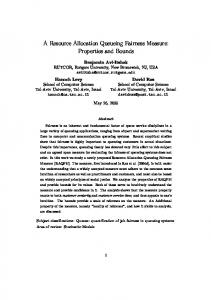
The choice of 1/(1 − ρ) is justified mainly because PS is considered fair, and thus any job size which is treated at least as good as the way it is treated under PS is treated fairly. Wierman [152] provides more formal reasoning. Definition 2.2. Let 0 < ρ < 1 in an M/GI/1 queue where X is non-deterministic. A scheduling policy P is: (i) Always Fair if P is fair for all such ρ and X; (ii) Sometimes Fair if p is fair under some ρ and X and unfair under other ρ and X; or (iii) Always Unfair if P is unfair under all loads and service distributions. The results of this classification for a wide set of scheduling policies are summarized in Figure 2.1 (the figure is from Wierman [152], brought with permission of the author).

Figure 2.1: Classification According to the Expected Slowdown Fairness Criterion

Another approach based on the slowdown is the Slowdown Queueing Fairness measure, SQF, proposed in Avi-Itzhak et al. [9]. SQF is based on the idea of equal slowdown, where deviation from equal slowdown is interpreted as unfair. Consider a system in equilibrium where service requirements are distributed as a random variable B with probability density function (pdf) b(x) and moments bk = E{B k }. Let T denote the equilibrium sojourn time and let T (x) denote the conditional sojourn time for a customer whose service requirement


12

is x. Absolute fairness is obtained when T (x) = cx, for some constant c which is chosen to in a way that guarantees zero sum. This leads to the following definition: Definition 2.3. The slowdown queueing fairness measure is the second moment of T (x) around cx:

Z SQF =

E{(T (x) − cx)2 }b(x)dx

where c = E{T }/b1 . The authors prove that unlike other fairness measures based on the slowdown, SQF accounts well for both seniority and size. For the M/GI/1 model the authors study non size-based policies and show that SQF F CF S < SQF ROS < SQF LCF S and SQF P S ≤ SQF P −LCF S . For the M/M/1 and M/D/1 models they also show that SQF LCF S = SQF P −LCF S and SQF LCF S < SQF P −LCF S , respectively. For other policies they provide simulation results that suggest that the measure always increases when the variability increases. Further, when variability is very high, SRPT and PS are the most fair amongst the policies compared. 2.1.3 Discrimination Frequency Measures Sandmann [136] presents an approach based on accounting for both service size and seniority explicitly, unlike other measures we surveyed which do so implicitly, if at all. Under that approach a customer is discriminated if either other customers are served earlier although they did not arrive earlier, or if the customer has to wait for customers with large service requirements. These two forms of discrimination are called overtaking and large jobs, respectively. Definition 2.4. Let ni , the amount of overtaking a job Ji suffers from, be the number of jobs that arrived not earlier and complete service not later than Ji . Let mi , the amount of large jobs a job Ji suffers from, be the number of jobs not completely served upon arrival of Ji that have at least as much remaining service requirements, and complete service not


13

later than Ji . The discrimination frequency of a job is def

DF (i) = ni + mi . The fairness of a system is defined by taking expectations over the discrimination frequency of an arbitrary job in steady state, i.e.

E{DF }.

It is easy to see that the measure accounts (explicitly) for both seniority and size, and this is further emphasized in Sandmann [136]. In Sandmann [134] the measure is evaluated for FCFS, LCFS and SJF. For the M/M/1 model it is analytically shown that

E{DF }SJF < E{DF }F CF S < E{DF }LCF S . Using simulation, the authors show that this is not the case with other service requirement distributions, where sometimes FCFS is more fair than SJF. In Sandmann [135] the author proposes a service policy which he shows by simulation to be more fair than both FCFS and SJF.

2.2 Fairness Measures in Related Areas Fairness has been excessively treated in computer and communication science in contexts different than that of job fairness. When we relate to jobs we have specific customers in mind, arriving at the system, receiving service, and departing. This is not the case with the following related areas of research. The first related area, where several fairness measures were proposed, is flow control. The best known notion in this area is that of Max-Min Fairness, starting with Jaffe [70, 71] and used by many afterwards. According to this concept a flow control scheme is fair if “each user’s throughput is at least as large as that of all other users which have the same bottleneck.” Gerla and Staskauskas [54, 55] achieve fairness by minimizing an objective function which was originally suggested by Gallager and Golestani [52], which includes a penalty for uneven allocation. Bharath-Kumar and Jaffe [17] state that any algorithm which allocates


14

zero throughput to any user is unfair; otherwise it is fair. Marsan and Gerla [98] present a quantitative fairness measure F = min i,j

pi , pj

where pi and pj are the powers (ratio of throughput and round trip delay) achieved by users i and j respectively. A protocol is called optimally fair if F = 1. Sauve et al. [137] contends that the fairness of a network should be measured by the variance of network delays of the different classes. This is revised to squared coefficient of variation of delay by Wong and Lam [158] and to a weighted squared coefficient of variation in Wong et al. [159]. Almost two decades later, the research area flourished again with the proposal of Proportional Fairness by Kelly [80], Kelly et al. [81]. Lately Balanced Fairness (Bonald and Proutière [20, 21]) and (p, α)-Proportional Fairness (Mo and Walrand [100]) were proposed. See survey of results in Roberts [126] and a comparative study in Bonald et al. [22]. The measures in this area assume some flow requirements exist in a network, and focus on the amount of bandwidth each flow should receive. The assumption is that the requirements and bandwidth assignments are permanent, and there is little significance to the order in which specific jobs arrive; only the overall bandwidth matters. As such they cannot be readily applied to the models we are interested in. An interesting recent paper on the subject, Briscoe [26], claims that comparing flow rates should not be used for claims of fairness in production networks. Instead, one should judge fairness mechanisms on how they share out the ‘cost’ of each user’s actions on others. A second related area is that of stream fairness. Within that context, the literature has flourished on the subject of Fair Queueing, which received very much attention in the recent decade. Fair Queueing disciplines (starting with Demers et al. [43, 44]), and their variants, aim at the fair scheduling of packet streams within network devices. The most prominent measures in this area are the Absolute Fairness Bound (AFB) and Relative Fairness Bound (RFB). AFB, first used probably in Greenberg and Madras [59], is based on the maximum difference between the service received by a flow under the discipline being measured, and the service it would have received under the ideal PS policy. As AFB


15

is frequently hard to obtain (see Keshav [82], ch. 9) RFB was proposed, first used probably by Golestani [57]. RFB is based on the maximum difference between the service received by any two flows under the policy being measured, see Zhou and Sethu [162] for relations between AFB and RFB. A similar criterion was suggested by Friedman and Henderson [50]. According to that criterion, a protocol p is considered fair if it weakly dominates PS, namely no job completes later under p than under PS, on any sample path. This criterion is similar to AFB in that it compares the protocol against PS, and it considers the worst case scenario, though it only classifies the protocol as fair or unfair. Most works in this area are based on the concept that General Processor Sharing (GPS) provides fair treatment to streams and thus policies “close” to GPS are fair as well. Some examples of early papers on the subject are Parekh [109], Parekh and Gallager [110, 111], Rexford et al. [125], Bennet and Zhang [15]. Many other papers have been published on the subject. Although these measures were originally meant to be used in studying flows and not specific jobs, they can be applied to jobs as well. For example, for AFB one can compute the maximum difference between the departure time of each job and the departure time it would have received under PS. However, when either of these measures is used for evaluating job fairness, the following emerges: 1. If job sizes are unbounded, these measures are unbounded (i.e. infinitely unfair) for all non-preemptive policies. In fact, the tightest bound possible for any nonpreemptive policy is the size of the largest job, achieved by the Fair Queueing policy proposed in Demers et al. [43, 44]. 2. Even if job sizes are bounded, it is easy to see that these measures do not differentiate between many non-preemptive service policies. For example, both FCFS and LCFS are equally and infinitely unfair, and so are most other non-preemptive policies. Both cases above imply that these measures, based on a maximal-difference approach are not sensite enough to differentiate between many popular scheduling policies which drastically differ from each other.


16

In the area of load balancing, Wang and Morris [149] propose the Q-factor. The Qfactor measures for a load ρ the mean response time of the worst customer source under the worst possible combination of stream loads, compared to the mean response time under global FCFS (namely FCFS among the customers of all sources). It therefore describes how closely a system comes to a multi-server FCFS system, as seen by every job stream. Another area where related works are starting to appear is parallel job schedulers. Sabin et al. [131] propose a notion in which a job has been treated unfairly if its start time is delayed because of a later arriving job, not taking the job size into account. The results in this work are based on simulation. The work in Sabin and Sadayappan [130] provides another two unfairness metrics, one based on Gordon [58] (discussed above), and one based on RAQFM. The results in this work were also based on simulation. Vasupongayya and Chiang [148] use the variance, and other simple summary metrics, of some simplistic performance metrics e.g. the waiting time or the job rate. Like the above works, the results are based on simulation.

2.3 Fairness Measures in General Fairness measures are also abundant in areas far from computer science. In the field of economics, one measure worth mentioning is the well known Gini Coefficient, published as early as 1912 in Gini [56]. The Gini Coefficient is a measure of R1 inequality of a distribution of income. It is formally defined as 1 − 2 0 L(x)dx, where L(x) is the function representing the Lorenz curve (Lorenz [95]). In some cases it can also be calculated without direct reference to the Lorenz curve, see Gastwirth [53], Dorfman [45]. We have tried to apply the Gini Coefficient to our model, but as the “income” from the system is unclear, and varies with time this proved to be too complicated. However, the principles are not entirely unconnected. Although strictly speaking the Fairness Index proposed in Jain et al. [73] was suggested in the context of computer systems, and was motivated by the research in the area of flow control, it is aimed at fairness of resource sharing in general. The four desired properties


17

of such an index, according to the authors, are (1) Population size independence, (2) Scale and metric independence, (3) Boundedness between 0 (totally unfair) and 1 (totally fair) and (4) Continuity. Assuming a vector of basic metrics x = (x1 , . . . , xn ), xi ≥ 0 their measure is

P ( ni=1 xi )2 . d(x) = Pn n i=1 x2i

By choosing the right basic metrics the same index can be applied to any setting. Algorithms for optimizing the Fairness Index are studied in Raftopoulou et al. [114]. Another field in which evaluating fairness is of interest is consumer reaction, where measurement is usually done through customer satisfaction surveys. Carr [29] proposes FAIRSERV - a model for evaluating consumer reactions to services based on a multidimensional evaluation of service fairness. Fairness is evaluated through five distinct fairness constructs, which are discussed in the fairness literature: distributive, procedural, interpersonal, informational, and systemic or overall fairness. All involve perceptions of the fairness of specific entities and activities.

Chapter 3 MODEL AND NOTATION

In this work we address quite a number of models, each requiring its own notation. To ease the reading, most of the notation related to each of the models is presented when the model is introduced. In this chapter we only summarize some of the common elements in these models, and the general notation practices we use. We also describe the common service policies investigated in this work.

3.1 Customers and Scenarios Consider a system which is subject to the arrival of a stream of customers, C1 , C2 , . . . , who arrive at this order. Let si , ai , di , denote the service requirement measured in time units, the arrival epoch, and the departure epochs of Ci , respectively. Specific series of values are called an arrival pattern ({ai }i=1,2,...,L ), an arrival and service pattern ({ai , si }i=1,2,...,L ), and a scenario ({ai , si , di }i=1,2,...,L ). Applying a service policy on an arrival and service pattern creates a scenario. We limit our discussion to arrivals which are independent of the system state and server decisions. At each epoch t the system grants service at rate of si (t) ≥ 0 to Ci . The system is Rd work-conserving, i.e. aii si (t)dt = si . The total service rate given by the system is denoted def

s(t) =

P

i si (t)

≥ 0. Let N (t) denote the number of customers in the system at epoch t.

Unless otherwise specified, all customers are “born equal”, belonging to the same class of customers, and thus no weights are assigned to them. Throughout this work we use ρ in its common definition as the system utilization

Chapter 3. Model and Notation

19

def

factor, which is ρ = λ¯ x/M where λ is the average arrival rate, x ¯ is the average service requirement, and M is the number of servers (e.g. Kleinrock [88], Sec. 2.1). For stability, we usually assume ρ < 1.

3.2 Classes of Service Define Φ to be the class of non-preemptive, non-divisible service polices, i.e. service policies where once the server started serving a customer it will not stop doing so until the customer’s service requirement is fulfilled, and at most one customer is served at any epoch by each server. Define Φ∗ to be a subclass of Φ including only policies where the scheduler does not account for the actual values of the service requirements in the service decisions. Note that service policies may depend on the whole history of service, and particularly on how many jobs are in the system. On the other hand, if customers are assumed to all belong to the same class, policies belonging to Φ∗ cannot distinguish between customers at all based on size, not even by broad classifications such as ‘small’ and ‘large’.

3.3 General Notation Practices We use Typrwriter-Style to denote scheduling policies. For convenience, we sometimes use the notation X (i) to denote the i-th moment of X, def

i.e. X (i) =

b do denote E{X i }. We also use bar (X) to denote expected value and hat (X)

variance. We use 1(¦) to denote the indicator function, i.e. ( 1 1(¦) = 0

the expecssion ¦ is true . otherwise

We use Bold − Style to denote vectors, e.g. X. We use angled brackets, e.g. ha, bi, to denote a state of a system.


20

3.4 Common Service Policies In this section we define some common service policies used in this work, and mention some commonly known performance results. PS: Processor Sharing Under PS the processor is shared among all jobs currently in the system, in equal shares. FCFS: First Come First Served Under FCFS the jobs are served in the order of arrival. Also sometimes referred to as FIFO for First In First Out. LCFS: Last Come First Served Under LCFS the jobs are served in the opposite order of arrival, but without preemption. Also sometimes referred to as LIFO for Last In First Out. P-LCFS: Preemptive Last Come First Served Under P-LCFS the jobs are served in the opposite order of arrival, and an arriving job preempts the currently served job. SRPT: Shortest Remaining Processing Time First Under SRPT at every moment of time, the server is processing one of the jobs with the shortest remaining processing time (usually chosen in random if more than one such job is available). The SRPT policy is well-known to be optimal for minimizing mean response time (Schrage and Miller [139], Schrage [138]). LAS: Least Attained Service Under LAS the job which received the least service gets the processor to itself. If several jobs all have the least attained service, they time-share the processor via PS. Also sometimes referred to as FB for Forward-Backward or FeedBack, or SET for Shortest Elapsed Time. See Nuyens and Wierman [103] for a recent survey of history and results. LRPT: Longest Remaining Processing Time First Under LRPT at every moment of time, the server is processing the job with the longest remaining processing time. If multiple jobs in the system have the same remaining processing time, they time-share the processor via


21

PS. Note that this means that a job can only leave the system at the latest time possible, which is the end of the busy period. Thus it is probably the worst service policy possible in terms of efficiency. ROS: Random Order of Service Under ROS whenever the server becomes idle, one of the customers in the system is chosen for service in a uniformly random way. P-ROS: Preemptive Random Order of Service Under ROS whenever the server becomes idle, or a new customer arrives, one of the customers in the system is chosen for service in a uniformly random way. SJF: Shortest Job First Under SJF the jobs are served in order of service requirement, starting with the smallest, without taking into account the amount of service already given. LJF: Longest Job First Under LJF the jobs are served in order of service requirement, starting with the largest, without taking into account the amount of service already given. P-SJF: Preemptive Shortest Job First Under P-SJF the jobs are served in order of service requirement, starting with the smallest, without taking into account the amount of service already given. An arriving job preempts the currently served job if it has shorter service requirement. P-LJF: Preemptive Longest Job First Under P-LJF the jobs are served in order of service requirement, starting with the largest, without taking into account the amount of service already given. An arriving job preempts the currently served job if it has longer service requirement. RR: Round Robin Under RR customers are served in a cyclic manner, where in each cycle each customer receives a service quantum ∆. To avoid system idling it is usually assumed


that service requirements are integer multiples of ∆.

22

Chapter 4 INTRODUCING THE FAIRNESS MEASURE: RAQFM

In this chapter we introduce the fairness measure we propose, RAQFM: a Resource Allocation Queueing Fairness Measure. Before proposing a fairness measure, one needs to ask the question, what is fairness? While almost every child, if asked, can tell you what is fair and what is not, it is quite a demanding undertaking to have a group of people agree on a common definition of fairness, much more so when it comes to defining a quantitative measure of the level of fairness. Our approach in this is to consider the queueing system as a microcosm social construct. Its fairness should therefore conform to the general cultural perception of social justice in the particular society. The issue of fairness and social justice has always been, and still is, a cardinal issue in all cultures. It is the cement holding the society together and as such it has been subject to debate by philosophers, prophets and spiritual leaders since the beginning of recorded history. Maybe one of the first relevant formulations of this issue is Aristotle’s idea in “Nicomachean Ethics”, that justice consists, at least in part, in treating equal cases equally, and unequal cases in proportional manner (Aristotle [4], Book V): “Also, there will be the same equality between the persons and the shares: the ratio between the shares will be the same as that between the persons.” In modern time, many economists and social scientists joined the ongoing debate. As is to be expected, there is a vast ocean of modern research and publications on this issue, mostly by philosophers, economists and social and behavioral scientists. It is of course be-

Chapter 4. Introducing the Fairness Measure: RAQFM

24

yond the scope of this work to review and interpret this literature, see some comprehensive reviews of the justice and fairness literature in Cropanzano [37], Beugré [16], Folger and Cropanzano [49], Cohen-Charash and Spector [33], Colquitt et al. [34], Cropanzano et al. [38]. However, a most prominent and comprehensive publication on this issue is Rawls’ book “A Theory of Justice” (Rawls [115]). In essence, Rawls’ general conception of social justice is (Rawls [115], p. 303): “All social primary goods - liberty and opportunity, income and wealth, and the bases for self-respect - are to be distributed equally unless an unequal distribution of any or all of these goods is to the advantage of the least favored.” We therefore see that throughout the debate, one prominent concept is that of fair resource allocation, or the idea that fairness is achieved when the resource ‘pie’ is appropriately divided between the consumers. But what is the pie in the case of a queueing system, and how should it be divided? A very similar concept in the area of queueing is that of Processor Sharing, as embodied by the ideal PS policy, analyzed as early as Kleinrock [86, 87], Coffman et al. [32]. The root idea of this policy is that at every moment of time, the service rate is divided equally amongst the jobs present in the system. This leads us to the basic principle, or belief, which is in the roots of our proposed measure: At every epoch all jobs present in the system deserve an equal share of the system’s service rate. Deviations from it creates discriminations (positive or negative). Accounting for these discriminations and summarizing them yields a measure of unfairness. The process for measuring RAQFM is therefore composed of two distinctive parts: 1. Discrimination: Each customer is given a single measure representing how well the customer was treated. A positive numbers mean the customer was well treated, and a negative number means the customer was not treated well.


25

2. Fairness: A summary measure is taken over the discriminations. The (non-negative) result of this summary measure is the system’s unfairness, so a low measure means a more fair system.

4.1 RAQFM For Single Non-Idling Server We start with the description of RAQFM for a single non-idling server, as first proposed in Raz et al. [117]. Observe a single server system, with a service rate of one unit. The server is non-idling, P i.e. ∀t, N (t) > 0 ⇒ i si (t) = 1. 4.1.1 Individual Customer Discrimination As the principle implies, at every epoch t, all customers present in the system deserve an equal share of the system resources, or 1/N (t). We call this quantity the warranted def

service rate of Ci at epoch t, and denote it Ri (t). Integrating this for Ci yields Ri = R di ai dt/N (t), the warranted service of Ci . The (overall) discrimination of Ci , denoted Di , is the difference between the warranted service and the granted service, i.e. Z Di = si − Ri = si −

di

ai

1 dt N (t)

(4.1)

A positive (negative) value of Di means that a customer receives better (worse) treatment than it fairly deserves, and therefore it is positively (negatively) discriminated. An alternative way to define Di is to define the instantaneous discrimination rate of Ci at epoch t, def

δi (t) = si (t) −

1 , N (t)

(4.2)

and then the overall discrimination of Ci is: Z Di =

di

ai

δi (t)dt.

(4.3)


26

An important property of the discrimination is that it obeys, for every non-idling workP conserving system, and for every t: i δi (t) = 0, that is, every positive discrimination is balanced by negative discrimination. This results from the fact that when the system P P is non-empty i si (t) = 1 (due to non-idling) and i Ri (t) = N (t)(1/N (t)) = 1. An important outcome is that if D is a random variable denoting the discrimination of an arbitrary customer under steady state, then E{D} = 0, namely the expected discrimination of an arbitrary customer under steady state is zero. A complete proof is given in Section 5.3. The reason we use the total discrimination, rather than maybe the average instantaneous discrimination, i.e. the total discrimination divided by the sojourn time, is twofold. First, it represents better the effect a customer has on the system’s resources. A customer which takes a non-proportionally large share of the service rate for a long period of time, effects the system more than a customer which does the same for a short period of time. Second, it represents better the perception a customer has of the system. A customer receiving less than a fair share of the service rate for a long period of time is more likely to have a negative perception of the system than one receiving such unfair share for a short period of time. 4.1.2 System Measure of Unfairness As mentioned above, to measure the unfairness of a system and of a service policy across all customers, that is, to measure the system unfairness, one would choose some summary statistics measure over D, where D is a random variable denoting the discrimination of an arbitrary customer when the system is in steady state. Since fairness inherently deals with differences in treatment of customers, a natural choice is the variance of customer b As E{D} = 0, this equals the second moment, that is E{D2 }, denoted discrimination, D. FD2 . Another optional measure is the mean of distances E{|D|}, denoted F|D| . One can also choose to ignore customers with positive discrimination and use the mean value over customers with negative discrimination, −E{D | D < 0}. However,


27

note that in some cases this might not be meaningful. For example suppose D1 = D2 = · · · = D19 = 1 and D20 = −19, then −E{D | D < 0} = 19. In other words, using the mean value over customers with negative discrimination might lead to very few customers influencing the unfairness in a major way. What might be more correct is the average negative discrimination, assuming positive discrimination does not count, but averaging

E{min(D, 0)} which in this case equals 19/20 = 0.95. However, E{min(D, 0)} = E{max(D, 0)} = E{|D|}/2 = F|D| /2. over all customers, i.e.

Another approach is to use higher central moments, E{(D− E{D})k }, which in this case are equal to the moments E{Dk }. Alternatively one can use cumulant moments (see textbook Bailey [12] or examples of use Choudhury and Whitt [31], Duffield et al. [46], Matis and Feldman [99], Wierman and Harchol-Balter [154]). In fact, summary functions for variability or fairness have been suggested in other fields as well, see Chapter 2, e.g. the Fairness Index (Jain et al. [73]), and many of them will do. We believe that the choice of summary function is of less importance, and we choose to focus on the simplest ones, FD2 and F|D| . Throughout this work, the term “unfairness” refers to FD2 . 4.1.3 Unfairness of a Scenario Recall that a scenario is defined as a specific series of values ({ai , si , di }i=1,2,...,L ). The unfairness of a scenario is also defined by some summary statistics measure over the set of individual discriminations Di , i = 1, . . . , L. A natural choice is the statistical variance of customer discrimination, and since the average of Di is zero, this equals the statistical P 2 second moment, that is L1 L i=1 (Di ) , denoted FD2 . Similarly other optional measure are 1 PL 1 PL i=1 |Di | (denoted F|D| ) or L i=1,Di d0k , then all departures up to d0k are the same for PS and for φ, and therefore ∀t < d0k , N 0 (t) = N (t). Thus, Z Dk0

= sk −

d0k

ak

Z 0

dt/N (t) = sk −

d0k

ak

ÃZ dt/N (t) = sk −

dk

Z dt/N (t) −

d0k

ak

Z =

dk

dk

! dt/N (t)

dt/N (t) > 0,

d0k

as N (t) ≥ 1 in (d0k , dk ) since Ck is in the system. Thus, the assumption is contradicted. Now suppose dk < d0k , then all departures up to dk are the same for PS and for φ, and therefore ∀t < dk , N 0 (t) = N (t). Thus, ÃZ Dk0 = sk −

dk

ak

Z dt/N 0 (t) +

d0k

! dt/N 0 (t)

dk

ÃZ = sk −

dk

Z dt/N (t) +

ak

d0k

! dt/N 0 (t)

dk

Z =−

d0k

dt/N 0 (t) < 0,

dk

again contradicting the assumption. Theorem 5.4 (Absolute Fairness in Multiple Server Systems). The above theorem also applies to (i) PS in multiple server systems and (ii) the G/G/∞ model.

Chapter 5. Basic Properties of RAQFM

42

Proof. (i) When applying the above theorem to multiple server systems one needs to first define its exact operation. One ideal way to define PS in a system with M servers is that if N (t) ≤ M then each customer is served by one server. Otherwise, each customer receives a service rate of M/N (t). Thus ( 1

si (t) = and

M N (t)

( ω(t) =

N (t) ≤ M , N (t) > M

N (t) N (t) ≤ M . M N (t) > M

Using the definition of δi (t) in (4.4) ω(t) δi (t) = si (t) − = N (t)

( 1− M N (t)

N (t) N (t)

−

=0

M N (t)

N (t) ≤ M

= 0 N (t) > M

= 0.

(ii) in the G/G/∞ mode si (t) = 1 and ω(t) = N (t). Using (4.4) δi (t) = 1−N (t)/N (t) = 0. The rest of the proof, in both cases, is identical to the proof of Theorem 5.3 Note that this does not depend on the system being non-idling or work-conserving.

5.3 Zero Sum Theorem 5.5 (Zero Expected Value). In a stationary system, the expected value of discrimination always obeys E{D} = 0. Proof. Observe that the total momentary discrimination rate at any epoch t is X {i|ai 0)˜ µd(a − 1, b).

(7.2)

(4) Similarly, the equations for d(2) (a, b) are ˜ (2) (a, b + 1) + 2t(1) δ(a, b)λd(a, ˜ d(2) (a, b) = t(2) (δ(a, b))2 + λd b + 1)+ ³

´

1(a > 0) µ˜d(2) (a − 1, b) + 2t(1) δ(a, b)˜µd(a − 1, b) . (7.3)

Chapter 7. Computing RAQFM Under The Markovian Model

70

(5) The states possible upon arrival are hk, 0i, k = 0, 1, . . . , where k is the number of customers seen on arrival. Therefore FD2 =

∞ X

pk d(2) (k, 0),

(7.4)

k=0

where pk = (1 − ρ)ρk is the steady state probability of encountering k customers in the system.

(7.5)

Chapter 8 FAIRNESS IN SINGLE SERVER SYSTEMS

In this chapter we use RAQFM to analyze the unfairness of several service disciplines in single server systems, namely FCFS, LCFS, P-LCFS and ROS. We start with the M/M/1 paradigm. We derive the expected discrimination experienced by an arriving customer as a function of the number of customers it finds in the system upon arrival. The results shed light on customer discrimination as a function of the queue situation it encounters. We then derive the system unfairness, measured via the variance of discrimination, for these four policies. Most of this material in this section was published in Raz et al. [117]. Following that, we study other service requirement distributions. We use simulation to study a bi-valued distribution with high variability. We then present results from Brosh et al. [27] that studied general distributions, with focus on phase type ones.

8.1 Conditional Discrimination in M/M/1 In this section we consider an M/M/1 system with arrival rate λ and mean service length

E{D | k}, the expected customer discrimination, conditioned on the number of customers it finds in the system upon arrival. While E{D | k} is not used to

1/µ. We derive

derive the system unfairness, it is still an interesting measure that will serve to shed light on the situations at which systems are subject to high discrimination. The general method for this evaluation was already detailed in the previous section, see Remark 7.2.

Chapter 8. Fairness in Single Server Systems

72

8.1.1 FCFS The analysis of FCFS was detailed in Section 7.2, and (7.2) provides a set of equations for evaluating d(a, b). We can use E{D | k} = d(k, 0) to evaluate the conditional distribution. Remark 8.1. Note that the quantity E{D|k} depends on λ and µ only through their ratio t(1) ρ = λ/µ, and not through their individual values. This is true for all the policies studied in this chapter. Alternatively, one can compute E{D | k} using the result of the following theorem. Theorem 8.1. Let P (a, b | k) be the probability that a walk visits ha, bi given that the customer sees k other customers upon arrival and let G(a, b | k) be the number of times ha, bi is reached in in such a walk. Then (a) µ ¶ µ ¶ ρb k−a+b b k−a k − a + b ˜ P (a, b | k) = E{G(a, b) | k} = λ µ ˜ = , b (1 + ρ)k+b−a b and therefore (b)

E{D | k} = t(1)

k ∞ X X

P (a, b | k)δ(a, b),

(8.1)

b=0 a=0

Proof. Moving along a walk b is monotone non-decreasing and a is monotone non-increasing. Furthermore, either the value of a of the value of b must change by one unit in each step. Therefore, if ha, bi is visited, it cannot be visited again, and thus the range of G(a, b | k) is {0, 1} and

E{G(a, b) | k} = P{G(a, b | k) = 1} = P (a, b | k). This proves the first equality of (a), and (b) follows immediately. To prove the rest of (a) we note that a walk will do this if and only if the first k − a + b events in the walk consist of exactly b arrival events and k − a departure events. The probability of such a walk is given by the binomial distribution: µ ¶ µ ¶ ρb k−a+b b k−a k − a + b ˜ E{G(a, b) | k} = λ µ˜ = , b (1 + ρ)k+b−a b


73

def ˜ def where for the second equality recall that λ = λ/(λ + µ), µ ˜ = µ/(λ + µ).

Special Cases

E{D | 0}, the expected discrimination for a customer arriving at an empty system can be easily derived from (8.1):

E{D | 0} = t

(1)

∞ X b=0

1 λ (1 − ) = t(1) b+1 ˜b

Ã

∞ X ˜b 1 λ − ˜ b+1 1−λ b=0

!

The second part of this sum yields: Z ∞ Z ∞ ∞ ˜ b+1 ∞ Z X ˜b λ 1 1Xλ 1 X ˜b ˜ 1 X ˜b ˜ 1 ˜ λ dλ = = = λ dλ = dλ ˜ ˜ ˜ ˜ ˜ b+1 b+1 λ λ λ λ 1 − λ b=0 b=0 b=0 b=0 =

1 ˜ ln(1 − λ), ˜ λ

and so µ

E{D | 0} = t(1)

¶ ¶ µ 1 1 ˜ = t(1) 1 + ρ + 1 + ρ ln 1 + ln(1 − λ) ˜ λ ˜ ρ 1+ρ 1−λ µ ¶ 1+ρ (1) =t 1+ρ− ln(1 + ρ) . ρ

Observe that E{D | 0} is a monotone-increasing function in ρ and thus its maximum value is reached when ρ → 1 and its minimum value is reached when ρ → 0, the high and low traffic bounds. For the high traffic bound ρ→1

E{D | 0} −−−→ t(1) (2 − 2 ln 2) ≈ 0.613706t(1) ,


74

which is the maximum expected discrimination for a user in the FCFS service policy. For the low traffic bound

E{D | 0} = t

(1)

µ ¶ 1+ρ 1+ρ− ln(1 + ρ) ρ µ ¶ 1 ρ→0 (1) =t 1 + ρ − ln(1 + ρ) − ln(1 + ρ) −−−→ t(1) (1 + 0 − 1) = 0. ρ

This is expected since when ρ → 0 there are almost no arriving customers, thus an arriving tagged customer finding the system empty will be served immediately, and leave without experiencing arrivals during its stay. Thus, its discrimination approaches D = 0. Another value easily derived is the limit of E{D | k} for ρ → 0. If ρ → 0 it follows ˜ → 0 and µ immediately that λ ˜ → 1 and thus E{G(a, b) | k} = 0 for b > 0 and so (8.1) becomes ρ→0

E{D | k} −−−→ t

(1)

k X

δ(0, a) = 0 + t

a=0

(1)

k X a=1

−

1 = −t(1) Hk , a+1

where Hn is the n-th harmonic number. For the numerical computation of other values using (8.1), the summation must be stopped at some large number, justified by the low probability of having very large values of b, i.e.

E{G(a, b) | k} −b→∞ −−→ 0. For the computation using (7.2) the same applies as

b→∞

d(a, b) −−−→ 0. This can be simply done by setting d(a, b) to be zero for large values of a and b. A second way to justify these is to look at a system with a large finite queue. Numerical results and properties Figure 8.1 depicts the value of the conditional discrimination normalized by t(1) , E{D|k} , t(1) as a function of k, for some values of ρ. We use the normalized discrimination due to Remark 8.1, which enables us to create a single plot that covers every value of both λ and µ, by creating a plot of ρ. We will follow this convention throughout this section.


75

All the special cases presented above can be verified in the figure. In addition we note the following properties: 1. The worst (most negative) discrimination a customer may experience is when the load approaches zero and the customer finds a very long queue; in this case the expected discrimination monotonically decreases in the queue length k and is unbounded. This seems to agree with common feelings where perhaps the most disappointing queue state one can encounter is a long queue when the load is very small. 2. The best (most positive) discrimination a customer may experience is to find an empty queue when the load is very high. This, again, seems to agree with common customer feelings. 3. Negative discrimination appears to monotonically increase with the queue size encounters. This seems to fit our intuition as well. 4. Normalized discrimination seems to monotonically decrease with the load ρ. 1

expectedfifo2.m

0.613706 0.5 0

E[D|k] / t(1)

−0.5 −1 −1.5 −2 −2.5 −3 0

ρ→1 ρ=0.8 ρ=0.5 ρ=0.2 ρ→0

5

10 k

15

20

Figure 8.1: Conditional (normalized) Discrimination for M/M/1 under FCFS


76

8.1.2 LCFS Following the same steps: (1) Let a ∈ N0 denote the number of customers ahead of C at the queue (and thus to be served after C). Let b ∈

N0 denote the number of customers behind C at the queue

(and thus to be served before C). (3) Possible events are: ˜ If C was in 1. A customer arrives into the system. The probability of this event is λ. service (b = 0) C’s state will change to ha + 1, bi, otherwise to ha, b + 1i 2. A customer leaves the system. The probability of this event is µ ˜. If C was in service, C will leave the system, otherwise C’s state will change to ha, b − 1i. This leads to the following set of equations: ( d(a, b) = t(1) δ(a, b) +

˜ λd(a, b + 1) + µ ˜d(a, b − 1) b > 0 . ˜ λd(a + 1, b) b=0

(8.2)

Observe that an arriving customer starts either with state h0, 0i when the system is empty, or with h1, k − 1i when it is not empty, thus (

E{D | k} =

d(k − 1, 1) k > 0 . d(0, 0) k=0

(8.3)

These equations can be solved numerically to evaluate E{D | k} The following is an alternative, more efficient, approach. We need Theorem 8.2 and Lemma 8.1 to prove Lemma 8.2, which will provide the actual method of evaluation. Theorem 8.2. Consider the infinite series an , bn , n = 1, 2, . . . defined iteratively as follows: a1 = 0

b1 = 1

a2 = t(1) c1,k + µ ˜d∗k

˜ b2 = λ


an =

n−2 an−1 + t(1) bn−1 cn−1,k − bn−1 µ ˜ abn−2

1−

bn−1 µ ˜ bn−2

77

=

bn−2 (an−1 + t(1) bn−1 cn−1,k ) − µ ˜bn−1 an−2 bn−2 − bn−1 µ ˜ ,n > 2

bn =

˜ n−1 λb 1−

bn−1 µ ˜ bn−2

=

˜ n−1 bn−2 λb bn−2 − bn−1 µ ˜

,n > 2

(8.4)

def

where cn,k = δ(k − 1, n) and Ã def d∗k = t(1)

∞ X ρ a 1 1+ρ− ) ( 1+ρ a+k

! .1

a=0

Then (i) d(k − 1, 0) = d∗k and (ii) for every n ≥ 1 and k > 0

E{D | k} = an + bn d(k − 1, n),

(8.5)

Proof. (i) d(k − 1, 0) can be evaluated according to (8.2) as follows ˜ ˜ (1) δ(k, 0) + λd(k ˜ d(k − 1, 0) = t(1) δ(k − 1, 0) + λd(k, 0) = t(1) δ(k − 1, 0) + λ(t + 1, 0)) = ··· = t

(1)

∞ X

˜ a−k δ(a − 1, 0) = t(1) λ

∞ X a=k

a=k

(

ρ a−k 1 ) (1 − ) 1+ρ a

Ã = t(1)

∞ X ρ a 1 1+ρ− ( ) 1+ρ a+k

! = d∗k .

a=0

(ii) For n = 1, follows immediately from (8.3). For n = 2, from (8.3) and (8.2) ˜ E{D | k} = d(k − 1, 1) = t(1) δ(k − 1, 1) + λd(k − 1, 2) + µ ˜d∗k , 1

d∗k can also be written as 1 + ρ − k1 F (k, 1; k + 1;

ρ ) 1+ρ

where F (a, b; c; x) is Gauss’s Hypergeometric

series, which might yield to even further reduction, see e.g. Jeffrey [75], Sec. 22.17, Abramowitz and Stegun [1], Sec. 15.1.


78

Next we prove the theorem for n ≥ 3 by induction. Induction base: correctness for n = 1, 2 was proven above. Induction assumption:

E{D | k} = am + bm d(k − 1, m) for m = 1, 2, . . . , n − 2, n − 1.

def

def

For brevity denote dn = d(k − 1, n) and cn = cn,k = δ(k − 1, n). Note that using this notation the assumption can be written as d1 = am + bm dm . Induction step: we now prove the correctness for m = n. From the assumption for m=n−2 d1 = an−2 + bn−2 dn−2 ⇒ dn−2 =

d1 − an−2 . bn−2

(8.6)

Note that using the abbreviated notation (8.2) for a = k − 1 can be written as follows ˜ n+1 + µ dn = t(1) cn + λd ˜dn−1 . Evaluating this at n − 1 yields ˜ n+µ dn−1 = t(1) cn−1 + λd ˜dn−2 . From the assumption for m = n − 1 d1 = an−1 + bn−1 dn−1 . Substituting dn−1 from (8.7) yields ˜ n+µ d1 = an−1 + bn−1 (t(1) cn−1 + λd ˜dn−2 ). Substituting dn−2 from (8.6) yields d1 − an−2 ˜ n+µ d1 = an−1 + bn−1 (t(1) cn−1 + λd ˜ ). bn−2 This leads to d1 (1 −

µ ˜bn−1 an−2 ˜ ) = an−1 + t(1) bn−1 cn−1 − µ ˜bn−1 + λbn−1 dn , bn−2 bn−2

(8.7)


79

and then d1 =

n−2 an−1 + t(1) bn−1 cn−1 − µ ˜bn−1 abn−2

1−

µ ˜bn−1 bn−2

+

˜ n−1 λb 1−

µ ˜bn−1 bn−2

dn ,

and by comparison to (8.5) the theorem is proved. Lemma 8.1. The series bn given above satisfies 0 < bn /bn−1 < ρ. n→∞

In other words, bn −−−→ 0. Proof. The proof is by induction. Induction base: for n = 2 ˜ = b2 /b1 = λ/1

ρ < ρ, 1+ρ

˜ > 0. and of course λ Induction assumption: 0 < bn−1 /bn−2 < ρ Induction step: From (8.4), bn can be written as bn =

˜ n−1 λb 1−

bn−1 µ ˜ bn−2

= 1

ρ 1+ρ bn−1 1 bn−1 1+ρ − bn−2

= ρbn−1

1 1+ρ−

bn−1 bn−2

.

From the assumption bn−1 1 bn−1 1⇒0< bn−2 bn−2 1+ρ− Substituting this in (8.8) yields 0 < bn < ρbn−1 proving the lemma.

bn−1 bn−2

< 1.

(8.8)


80

n→∞

Lemma 8.2. an −−−→ E{D | k} Proof. From Theorem 8.2 we have

E{D | k} = an + bn d(k − 1, n). From Lemma 8.1

n→∞

n→∞

bn −−−→ 0 while d(k − 1, n) is bounded. Thus an −−−→ E{D | k} This provides the actual way to evaluate E{D | k} iteratively, simply by computing an iteratively up to the required accuracy. Special Cases First note that for k = 0, all non-preemptive service policies yield the same results, thus

E{D | 0} = t

(1)

¶ µ 1+ρ ln(1 + ρ) , 1+ρ− ρ

ρ→1

E{D | 0} −−−→ t(1) (2 − 2 ln 2) ≈ 0.613706, ρ→0

E{D | 0} −−−→ 0.

(8.9) (8.10) (8.11)

It is also simple to evaluate E{D | k} when ρ → 0. In this case an arriving customer will almost surely wait for the current customer to be served, then be served herself, i.e. ρ→0

E{D | k} −−−→ t(1)

µ

1 1 +1− k+1 k

¶ =

t(1) (k 2 − k − 1) . k(k + 1)

Numerical results and properties , as a function Figure 8.2 depicts the conditional discrimination normalized by t(1) , E{D|k} t(1) of k, for some values of ρ. We note the following properties: 1. The highest value of negative discrimination is achieved at very high load and when k = 1. In this case the customer arrives and finds only the customer in service ahead of him, but then he ends up waiting for long time due to customers arriving after him. Thus a very high negative discrimination fits the natural intuition.


81

1.5

1

E[D|k] / t

(1)

0.5

0

−0.5

−1

ρ→0 ρ=0.2 ρ=0.5 ρ=0.8 ρ→1

−1.5

−2 0

5

10 k

15

20

Figure 8.2: Conditional (normalized) Discrimination for M/M/1 under LCFS

2. For all load values the highest value of negative discrimination is achieved when k = 1, which is, again, intuitive. 3. Relatively large values of positive discrimination are achieved when k is large. In these cases the arriving customer gets positively discriminated since it is served ahead of k − 1 of those customers. 8.1.3 P-LCFS Following the usual steps, we use the same state definition as in Section 8.1.2. (3) The possible events are ˜ C’s state will 1. A customer arrives into the system. The probability of this event is λ. change to ha, b + 1i 2. A customer leaves the system. The probability of this event is µ ˜. If C was in service, C will leave the system, otherwise C’s state will change to ha, b − 1i.


82

This leads to the following set of equations: ˜ d(a, b) = t(1) δ(a, b) + λd(a, b + 1) + 1(b > 0)˜ µd(a, b − 1). Observe that an arriving customer starts service immediately and thus

E{D | k} = d(k, 0).

(8.12)

Special Cases It is simple to evaluate

E{D | k} when ρ → 0. In this case an arriving customer will

almost surely be served in full and leave the system, thus ρ→0

E{D | k} −−−→ t

(1)

µ 1−

1 k+1

¶ k→∞

−−−→ t(1) .

Numerical results and properties , as a function Figure 8.3 depicts the conditional discrimination normalized by t(1) , E{D|k} t(1) of k, for some values of ρ. We note the following properties: 1. The highest value of negative discrimination is achieved at very high load and when k = 0. In this case the customer arrives and finds no customer in service ahead of him, but then he has a high chance of ending up waiting for long time due to customers arriving after him. Thus a high negative discrimination fits the natural intuition. 2. For all load values the highest value of negative discrimination is achieved when k = 0, which is, again, intuitive. 3. Relatively large values of positive discrimination are achieved when k is large. In these cases the arriving customer gets positively discriminated since it is served ahead of those k customers.


83

2

1

E[D|k] / t(1)

0

−1

−2

−3

ρ→1 ρ=0.8 ρ=0.5 ρ=0.5 ρ→0

−4

−5 0

5

10 k

15

20

Figure 8.3: Conditional (normalized) Discrimination for M/M/1 under P-LCFS

8.1.4 ROS (1) Let a ∈ N0 denote the number of customers in the system other than c. Let q ∈ {0, 1} be a boolean variable equaling 1 if the customer is in service and 0 if it is waiting. (2) From the state definition N (a, q) = a + 1, s(a, q) = q and δ(a, q) = 1(q = 1) −

1 . a+1

(3) Possible events are: ˜ C’s state will 1. A customer arrives into the system. The probability of this event is λ. change to ha + 1, qi. 2. A customer leaves the system, and C is chosen to receive service next. The probability of this event is µ ˜/a. C’s state will change to ha − 1, 1i. 3. A customer leaves the system, and C is not chosen to receive service next. The probability of this event is µ ˜(a − 1)/a. C’s change will change to ha − 1, 0i.


84

This leads to the following set of equations µ ˜ ˜ d(a, q) = t(1) δ(a, q) + λd(a + 1, q) + 1(q = 0) (d(a − 1, 1) + (a − 1)d(a − 1, 0)) . a Observe that a customer arrives at the system either at h0, 1i when the the system is empty, or at hk, 0i when it is not, thus (

E{D | k} =

d(0, 1) k = 0 . d(k, 0) k > 0

(8.13)

Special Cases Again, for k = 0 all non-preemptive service policies yield the same results (8.9)-(8.11). Numerical results and properties Figure 8.4 depicts the conditional discrimination normalized by t(1) , E{D|k} , as a function t(1) of k, for some values of ρ. We note the following properties: 0.8 ρ→1 ρ=0.8 ρ=0.5 ρ=0.5 ρ→0

0.6

E[D|k] / t

(1)

0.4

0.2

0

−0.2

−0.4

−0.6 0

5

10 k

15

20

Figure 8.4: Conditional (normalized) Discrimination for M/M/1 under ROS


85

1. The discrimination values are significantly lower (both positive and negative) compared to LCFS. This demonstrates the fact that ROS violates the natural service order (FCFS) significantly less than LCFS. 2. For all load values, the discrimination reaches zero when k is large. Recall that for PS discrimination value is constantly zero. This means that for large values of k ROS behaves like PS. We conjecture that this is even more so for preemptive variants of ROS.

8.2 System Unfairness in M/M/1 In this section we derive the system unfairness FD2 for the same four policies, under the M/M/1 paradigm. We will follow steps (4) and (5) from the method in Section 7.1. 8.2.1 FCFS The analysis FD2 for FCFS was already details in Section 7.2. (7.3) provides the set of equations for evaluating d(2) (a, b), (7.4) provides the arrival states and (7.5) provides their probabilities. 2 |k} also depends on λ and µ only Remark 8.2. Note that similarly to Remark 8.1, E{D t(2)

through their ratio ρ and thus can be computed from the knowledge of ρ alone. This is true for all the policies studied in this chapter. 8.2.2 LCFS (4) We get the following set of equations: d(2) (a, b) = t(2) (δ(a, b))2 ( +

³ ´ ˜ (2) (a, b + 1) + µ ˜ λd ˜d(2) (a, b − 1) + 2t(1) δ(a, b) λd(a, b + 1) + µ ˜d(a, b − 1) b>0 . ˜ (2) (a + 1, b) + 2t(1) δ(a, b)λd(a ˜ λd + 1, b) b=0


(5) Similarly to (8.3)

86

( d(2) (k − 1, 1) k > 0 , E{D | k} = (2) d (0, 0) k=0 2

and FD2 =

∞ X

pk E{D2 | k}

k=0

8.2.3 P-LCFS (4) We get the following set of equations: ˜ (2) (a, b + 1) + 2t(1) δ(a, b)λd(a, ˜ d(2) (a, b) = t(2) (δ(a, b))2 + λd b + 1) ³ ´ + 1(b > 0) µ ˜d(2) (a, b − 1) + 2t(1) δ(a, b)˜ µd(a, b − 1) . (5) Similarly to (8.12)

E{D2 | k} = d(2) (k, 0). 8.2.4 ROS (4) We get the following set of equations: ˜ (2) (a + 1, q) + 2t(1) δ(a, b)λd(a ˜ d(2) (a, q) = t(2) (δ(a, 0))2 + λd + 1, q) µ + 1(q = 0)

µ ˜(a − 1) (2) µ ˜ (2) d (a − 1, 1) + d (a − 1, 0) a a µ ¶¶ µ ˜ µ ˜(a − 1) +2t(1) δ(a, b) d(a − 1, 1) + d(a − 1, 0) . a a

(5) Similarly to (8.13) ( d(2) (k, 0) k > 0 E{D2 | k} = (2) . d (0, 1) k = 0


87

8.2.5 Numerical results and Discussion 12 Preemptive LCFS Non−Preemprive LCFS ROS FCFS PS

10

Var[D] / t

(2)

8

6

4

2

0 0

0.1

0.2

0.3

0.4

ρ

0.5

0.6

0.7

0.8

0.9

Figure 8.5: System Unfairness (Variance of Discrimination) for M/M/1

Figure 8.5 depicts

FD2 t(2)

as a function of ρ for the policies studied. The figure demon-

strates the following properties: 1. In terms of unfairness the policies may be ranked as P-LCFS > LCFS > ROS > FCFS > PS.

(8.14)

That is, P-LCFS is the most unfair and PS is the most fair. This dominance is observed for all values of ρ, except for ρ = 0. 2. At ρ = 0 the unfairness measures of all policies converge, as expected, and all policies experience full fairness, FD2 = 0. It is important to note that this results from the fact that most customers find an empty system upon arrival and thus are subject to no discrimination. Nonetheless if one conditions the discrimination on the system not being empty the discrimination is not zero.


88

3. The system unfairness seems to be monotonically increasing in the system utilization ρ for all policies. For FCFS and ROS the increase is modest, and the values at ρ = 0.9 are relatively low. In fact the slopes of their curves suggest that when ρ → 1 their values may converge to a finite number (in contrast, for example, to the expected delay, which blows up at ρ = 1). For LCFS and P-LCFS the increase is very drastic at high loads. At this point it is interesting to compare these results with other queueing fairness criteria, in particular the results derived in Wierman and Harchol-Balter [155], see Section 2.1.1 and specifically Figure 2.1. In that work PS and P-LCFS are shown to be “always fair”, while all non-preemptive, non-sized based policies, including FCFS, LCFS and ROS, are shown to be “always unfair”. Our results are in agreement regarding PS, which serves as the departure point for both measures, and regarding LCFS, which we find quite unfair. However, we differ significantly on FCFS and P-LCFS. The reason seems to be that the E{T (x)/x} classifier deals with the expected performance of a size-x job, averaged over all these jobs over all situations. The classifier emphasis is therefore on service requirements and it does not account directly for relative seniority. Thus P-LCFS whose seniority treatment is extremely unfair, as it discriminates against old jobs, is classified as fair, while FCFS whose seniority treatment is extremely fair is classified as unfair, maybe mostly because it is non-preemptive.

8.3 The Tradeoff Between Seniority and Service Requirements, and RAQFM’s Sensitivity To It The analysis of the M/M/1 system demonstrated that when the seniority differences dominate the service requirement ones, RAQFM properly ranks the policies by their seniority preferences. Our aim in this section is to demonstrate the sensitivity of RAQFM to service requirement discrepancies and show that when this factor dominates the seniority factor, RAQFM reacts properly. To this end we next consider a case where the arrivals remain Poisson while the vari-


89

ability of service requirements increases drastically. This is achieved by a bi-valued service requirement whose values are s = 0.1 with probability p and s0 = 10 with probability 1 − p. The value of p is selected to be p = 90/99 = 0.9009 so as to have mean service requirement of 1, identical to the previous numerical example. The variance of this service requirement is ps2 + (1 − p)s02 = 9.1, in comparison to the variance of the M/M/1 case which is 1/µ2 = 1. This system is analyzed via a simulation program, which was run on each evaluated point for at least 106 customers. Figure 8.6 depicts FD2 as a function of ρ for the FCFS, LCFS and P-LCFS policies. The figure demonstrates that over the range 35 Non−Preemptive LCFS FCFS Preemptive LCFS 30

25

F

D

2

20

15

10

5

0

0

0.1

0.2

0.3

0.4

ρ

0.5

0.6

0.7

0.8

0.9

Figure 8.6: System Unfairness For Discreet Distribution

ρ = (0, 0.55) RAQFM ranks P-LCFS as the most fair among the three policies, in contrast to its ranking in the M/M/1 case. As such, it concurs, in this case, with the ranking of the slow-down fairness approach in Wierman and Harchol-Balter [155] and is in contrast with the order fairness approach in Avi-Itzhak and Levy [7]. To understand this, note that due to the large variability of service requirements, large discriminations (and unfairness values) are formed when a large job is served and many small jobs queue behind it. In such cases preemption of large jobs from service can


90

alleviate this problem. P-LCFS achieves this since it tends to preempt the large jobs with high probability. Thus, in the case of high variability service requirements, where service requirement differences dominate seniority differences, P-LCFS can be more fair than FCFS due to giving preferential treatment to short jobs over long jobs, despite its preferential service to less-senior jobs over more-senior jobs. In summary, the examples presented in Figures 8.5 and 8.6 demonstrate how RAQFM accounts for the tradeoffs between seniority differences and service requirement differences. It should be noted that in the second example the lower unfairness of P-LCFS does not hold for the whole range of utilizations. For high load situations P-LCFS becomes again the most unfair policy. This may possibly be attributed to the fact that at high loads the queue size tends to be large and thus the magnitude of order discrepancies may increase sharply (similarly to the waiting time variance).

8.4 Going Beyond Exponential Service Requirement Lately, Brosh et al. [27] has researched RAQFM for single server systems, in more general settings, for the major purpose of researching the effect of variability on RAQFM. We bring here the major results of this work for completeness. Let S be a random variable denoting the service requirement of customer C, with first def

two moments s(1) and s(2) , variance σs2 and coefficient of variation γs = σs /s(1) . First, they analyze P-LCFS under a general M/G/1 model, and show that ·µ

E{D | k} = s

(1)

1 1− k+1

¶

¸ + λE{R | k + 1} ,

where R is the warranted service, recall from Section 4.1, and R | k is the warranted service conditioned on seeing k customers upon arrival, which they show to equals

E{R | k} = −

∞ s(1) X ρk+i+1 . ρk+1 k+i+1 i=0


91

The unfairness is FD2 = s(2)

∞ X

µ (1 − ρ)ρk 1 −

k=0

1 + λE{R | k + 1} k+1

¶2 +ρ

∞ X

(1 − ρ)ρk E{R2 | k + 1},

k=0

where E{R2 | k} can be evaluated using µ

E{R | k} = s 2

(2)

−1 + λE{R | k + 1} k+1

¶2

+ λs(1) E{R2 | k + 1}.

This shows that the unfairness of P-LCFS under M/G/1 is dependent only on the first two moments of the service requirement. For the rest of the service policies, FCFS, LCFS, ROS and P-ROS, the service distribution is approximated by a Coxian distribution using a second order moment matching technique (see Adan and Resing [2], Chap. 2). In particular, a phase-type distribution is fitted, either Coxian or Erlangian, to the mean s(1) and to the coefficient of variation γs . A distinction is made between two cases: (a) When 0 < γs < 1 the service requirement is matched to a k-stage Erlang distribution Ek and (b) When γs > 1 a Coxian-2 distribution is used which is composed of two exponential stages. The analysis of the system unfairness follows a method very similar to the one described in Section 7.1. We bring the analysis for a M/Er /1 system under FCFS as an example in Appendix C, compare with Section 7.2. Next, the effect of a long service customer, CL , on the discrimination in a nonpreemptive system is discussed. In the model observed CL has an exponential service requirement with parameter µ2 such that λ À µ2 . Time is slotted by arrivals and departures, and the probability of a slot ending with an arrival of another customer, rather than the departure of CL , is p = λ/(λ + µ2 ). It is shown that the expected negative discrimination observed by a small customer is at most ≈−

1 1 1 1 λ 1 ln( ) ≈ − ln( ) ≈ − ln( ), λ + µ2 1−p λ 1−p λ µ2


92

while the expected positive discrimination of CL is at most ≈

1 λ + µ2

µ

1 1 − ln( ) 1−p 1−p

¶ ≈

1 λ

µ

¶ λ λ − ln( ) . µ2 µ2

Interestingly the positive discrimination of CL is proportional to 1/µ2 while the negative discrimination of a customer is only proportional to its logarithm. Lastly, numerical results show the effect of variability. While for low variability the unfairness follows P-LCFS > LCFS > ROS > P-ROS ≈ FCFS > PS, which is identical to (8.14), for high variability LCFS ≈ ROS ≈ FCFS > P-LCFS > P-ROS > PS. The authors conclude that preemption is an instrumental tool for increasing fairness when job sizes variability is large.

8.5 Summary We studied four service disciplines under the M/M/1 regime: FCFS, LCFS, P-LCFS and ROS. For each of the service policies we derived the expected discrimination experienced by an arriving customer as a function of the number of customers it finds in the system upon arrival. We examined this behavior in detail for each of the service policies and the results were used to shed light on the behavior of the discrimination under these policies. Under the same settings, we derived the system unfairness, measured via the variance of discrimination, for the same four policies. Our results indicate that under exponential distribution the unfairness is monotonically increasing with the system load ρ, and the order of unfairness is P-LCFS > LCFS > ROS > FCFS > PS. We studied the behavior of the fairness for a bi-valued service distribution with large variability. The results showed that for this distribution, and under some loads, typically the not too high ones, P-LCFS can become more fair than LCFS and even FCFS, mainly due to preemption. We presented results from Brosh et al. [27], which studied general distributions and came to similar conclusions. Their study is an example of how to extend our analysis methods beyond the exponential service case.

Chapter 9 FAIRNESS OF MULTIPLES SERVER AND MULTIPLE QUEUE SYSTEMS

In this chapter we turn to investigate the fairness considerations in operating multiple server and multiple queue systems. We limit our discussion to servers with the same service rate, for simplicity a rate of one. Most of the material in this chapter was published in Raz et al. [122] and also appears in Raz et al. [119]. Multiple server queueing models have been used in a large variety of applications, including computer systems, call centers and Web servers, as well as human waiting lines, for example in airports. The configuration and operation of multi-server systems involves a variety of operational mechanisms that must be chosen. These include the number of queues and their dedication, the service policy, the queue joining policy and queue jockeying rules. An important motivation, perhaps the most important one, behind these multi-server mechanisms, is the wish to provide fair service to the jobs. The importance of these multiserver mechanisms, at least in the eyes of customers, was reinforced by psychological experimental queueing studies Rafaeli et al. [112, 113]. These experimental studies have further shown that the single-queue system is perceived to be more just (fair) compared to the multi-queue system. Our main purpose is to approve, in a quantitative manner, several rules of thumb that have been widely believed by practitioners and theoreticians but for which no analytic quantitative support was given. Particular design issues that we address are: 1) Whether to combine queues or not, 2) Whether to allow queue jockeying, and in what form, and 3) Queue joining policy.

Chapter 9. Fairness of Multiple Server Systems

94

Note that this is to our knowledge the first attempt to provide quantitative analysis of fairness for multi-queue multi-server systems; Most other fairness studies were limited to single server systems (the only exception we are aware of is Gordon [58]). The structure of this chapter is as follows. We start our analysis (Section 9.1) by considering G/D/m type systems, that is, systems with a general arrival process and deterministic service requirements. We study the queuing mechanisms mentioned above, i.e. combining queues, joeckeying, and queue joining policy. We then (Section 9.2) turn to study M/M/m type systems, namely systems with Poisson arrivals and exponential service requirements. We provide an exact fairness analysis for the same mechanisms, which demonstrates that in general the same properties shown for the G/D/m case hold also for the M/M/m one. We then (Section 9.3) turn to examine G/G/m type systems. We show, via some counter-examples, that the results derived in Section 9.1 and Section 9.2 do not necessarily hold for an arbitrary G/G/m model. We provide sufficient conditions under which some of them hold for the G/GI/m model. Another multi-server mechanism is that of combining servers. Although this issue could have been studied in this chapter, we chose to study it in the context of multiple class systems in Section 10.4, see there.

9.1 Fairness of G/D/m Type Systems In this section we analyze the fairness of G/D/m type systems, i.e. the customers arrive according to a general arrival process, the service requirements of all customers are identical, and the system has M servers. 9.1.1 The Effect of Seniority on Fairness We start with analyzing the effect of customer seniority on fairness, and show that under the G/D/m model serving customers in order of seniority increases system fairness. For simplicity we choose to demonstrate this for adjacently served customers. Consider two customers Cj and Ck that are adjacently served, i.e. they are scheduled to begin


95

service adjacently, with arrival times aj < ak and equal service requirements, i.e. sj = sk . Observe two possible cases: In the first case (Figure 9.1) they are served sequentially, by the same server. In the second case (Figure 9.2) they are served by two different servers in a partially-parallel manner. We have two possible schedules: In schedule (a), (Figure 9.1(a), Figure 9.2(a)), the order of seniority is preserved, i.e. Cj is served before Ck . In schedule (b), (Figure 9.1(b), Figure 9.2(b)), the order of service of Cj and Ck is interchanged and thus the order of seniority is violated. We assume that both of the schedules are possible, i.e. that Cj and Ck reside in the queue together for some time. Waiting

C

Service

j

Ck time

(a) Seniority Preserving Schedule

Cj Ck time

(b) Seniority Violating Schedule Figure 9.1: Case 1 - Sequentially Served Customers By The Same Server

Lemma 9.1 (Preference of Seniority Between Adjacently Served Customers with Equal Service Requirement). Let Cj and Ck be two customers, where aj < ak and their service requirements are equal, i.e. sj = sk = s. Then the unfairness (measured as FD2 ) of the seniority preserving schedule (a) is smaller than the unfairness of the seniority violating


96

Waiting

C

Service

j

Ck time

(a) Seniority Preserving Schedule

Cj Ck time E1

E2

E3

E4 E5

E6

(b) Seniority Violating Schedule Figure 9.2: Case 2 - Partially Parallel Served Customers

schedule (b), for every arrival pattern, regardless of the service requirements of the other customers. Proof. For simplicity we first prove this for adjacently served customers. We need to consider both cases. We note that the first case (Figure 9.1) was proven in Theorem 5.1, see Remark 5.1. We therefore only need to prove the second case (Figure 9.2). Let Dia and Dib denote the discrimination of Ci under schedule (a) and schedule (b) respectively. Let FDa 2 , FDb 2 denote the unfairness in the respective schedules, and let N a (t), N b (t) denote the number of customers in the system at epoch t, respectively. Let F˜ denote the total unfairness to all customers other than Cj and Ck , and let Fˆ denote the total unfairness to Cj and Ck . Then FD2 = Fˆ + F˜ . Define ∆FD2 , ∆Fˆ , and ∆F˜ to be the change, due to the interchange between Cj and


97

Ck , in the values of FD2 , Fˆ , and F˜ respectively. We need to prove that ∆FD2 ≥ 0, where ¤ 1£ b 2 ∆FD2 = ∆Fˆ + ∆F˜ = (Dj ) + (Dkb )2 − (Dja )2 − (Dka )2 L +

L L 1 h X b 2 X a 2i (Di ) − (Di ) , (9.1) L i6=j,k

i6=j,k

where L is the number of customers in the observed scenario. We divide the time interval (aj , max(dj , dk )) (namely from the arrival of Cj until both Cj and Ck depart) into five sub-intervals, where interval i, i = 1, 2, 3, 4, 5, is (Ei , Ei+1 ), and where E1 = aj ; E2 = ak ; E3 is the first point in time where service to either Cj or Ck starts; E4 is the point in time where service to the second customer starts; E5 = E3 + s; E6 = E4 + s (see Figure 9.2). As customers are adjacently served, E5 > E4 . We note that the number of customers in the system under schedule (a), N a (t), and the number of customers in the system under schedule (b), N b (t), are identical for every t. Therefore, the warranted service in interval i (of any customer) is the same in both schedules, and we denote it R(i) . As the warranted service in each interval is the same in both schedules, and as other customers’ departure epochs are also the same in both schedules, the interchange of Cj and Ck affects only Cj and Ck , i.e. Dia = Dib , i 6= j, k. Therefore ∆F˜ = 0, and from (9.1) it follows that ¤ 1£ b 2 ∆FD2 = ∆Fˆ = (Dj ) + (Dkb )2 − (Dja )2 − (Dka )2 L =

¢2 ¡ ¢2 1 £¡ s − (R(1) + R(2) + R(3) + R(4) + R(5) ) + s − (R(2) + R(3) + R(4) ) L

¡ ¢2 ¡ ¢2 ¤ 2 − s − (R(1) + R(2) + R(3) + R(4) ) − s − (R(2) + R(3) + R(4) + R(5) ) = R(1) R(5) > 0, L where the inequality is due to R(i) > 0, i = 1, 2, 3, 4, 5. This completes the proof for adjacently served customers. To address non adjacently served customers one has to address a third case, similar to case 1 where the service of the


98

second customer starts after the service completion of the first customer. The correctness of this case is very similar to that of case 1. Theorem 9.1 (Fairness of FCFS and LCFS under G/D/m). If the service requirements of all customers are identical, then for every arrival pattern, FCFS is the least unfair service policy in Φ and LCFS is the most unfair one. Note that by FCFS we mean global FCFS, i.e. serving customers by order of arrival. The proof is exactly the same as the proof of Corollary 5.1. 9.1.2 The Effect of Multiple Queues Operation Mechanisms on Fairness In this section we study the effect multiple queues mechanisms have on fairness, by observing several design and service decision considerations and examining their effect on the system fairness. One such decision is commonly referred to in the literature as the “Combining Queues” problem, in which a system consisting of M queues, each having service rate µ and arrival rate λ, and denoted the multi-queue system or the separate queue system, is compared to a system with one queue served by M servers with same service rate µ, and a corresponding arrival rate M λ, denoted the single queue system or the combined queue system. It is widely known that the single queue system is more efficient, i.e. it has a lower mean delay (a proof is given in Smith and Whitt [143]). However, if jockeying is allowed when a server is idle, in a manner that is nondiscriminatory with respect to the service requirement, the systems have the same mean waiting time. In other cases, for example when jockeying favors short jobs, the single queue system might even become less efficient than the separate queue system, see Rothkopf and Rech [129] for a full discussion in the matter. As mentioned above, in Rafaeli et al. [112, 113] an experimental psychology study showed that a single queue system is perceived to be more fair than a multiple queue one. Our goal is to quantitatively compare the fairness of the combined queue G/D/m system to that of the separate queue one. We show that indeed the combined (single) queue system is more fair than the separate (multiple) queue system.


99

A second issue, assuming multiple queues are used, is jockeying. In some systems jockeying is possible and we would like to find the effect it has on the system fairness. We focus on jockeying done while a server is idle, in a manner that is nondiscriminatory with respect to the service requirement. We leave other forms of jockeying for future research. The third issue, assuming jockeying is possible, is whether jockeying should be done from the head of the queue or from its tail. Note that from the efficiency (mean delay) point of view there is no difference between the two manners, as long as the jockeying is nondiscriminatory with respect to the service requirement. For the sake of illustration, we analyze four systems. All four systems have M servers. The first system has one common queue. A customer arriving at the system joins the tail of the queue, and when a server becomes free it serves the customer at the head of the queue, thus the system is non-idling1 . The customers are therefore admitted into service according to their order of arrival in a global FCFS manner. We refer to this system as the single queue system. The second system has M queues, where each of the servers serves only customers joining its assigned queue, in a FCFS manner. Customers arriving at the system are assigned to one of the queues in a uniformly random manner, and jockeying between the queues is not permitted at any time. We refer to this system as the standard multiple queue system. In Section 9.1.3 we address systems where queue joining isn’t done in a random manner. The third and fourth systems have M dedicated FCFS queues, and jockeying is allowed at epochs when a server is idle. Again, arriving customers are assigned to one of the queues in a uniformly random manner, however, if one or more of the servers is idle, an arriving customer is assigned to one of the idle servers, in a uniformly random manner. Following that, if a server becomes idle, a customer from one of the non-empty queues is immediately assigned to that server. The queue is chosen in a uniformly random manner, and the customer is chosen either from the head of the queue or from the tail of the queue. 1

A multi-server system is non-idling if the number of busy servers (and thus the actual service rate) is

always min(N, M ), where N is the number of customers in the system.


100

We refer to the first as the head-jockeying-on-idle multi-server system and to the second as the tail-jockeying-on-idle system. As mentioned above, both jockeying-on-idle systems are known to be as efficient as the single queue system, while the standard system is known to be less efficient than the other three systems. Theorem 9.2 (Single Queue is More Fair Than Multiple Queue for G/D/m). If the service requirements of all customers are equal, then for every arrival pattern, the single queue system has the lowest unfairness among the systems mentioned above. Proof. The proof is immediate since serving in a single queue means serving in a global FCFS manner, which is proven in Theorem 9.1 to be the most fair policy. Theorem 9.3 (Head-Jockeying-On-Idle is More Fair Than Tail-Jockeying-On-Idle for G/D/m). If service requirements of all customers are equal, and the choice of queue from which jockeying is done is identical, then for every arrival pattern the head-jockeying-onidle system has lower unfairness than the tail-jockeying-on-idle system. Proof. We prove that if the choice of queue from which jockeying is done is identical, the policy with the lowest unfairness is one where jockeying is always done from the head of the queue. Specifically, this proves that head-jockeying is more fair than tail-jockeying. We prove this by way of contradiction. Assume for the contradiction that there exists a jockeying policy ψ by which the jockeying customer is not always the customer at the queue head, and that ψ is the policy with the lowest unfairness for every arrival pattern. We will show that a policy with lower unfairness can be constructed. Consider an arrival pattern where there exists an epoch e in which a server was idle, and in which the customer admitted to the idle server by ψ was the n-th customer in some non-empty queue, and n > 1. Say there are N customers in that queue, and denote the customers in that queue C1 , C2 , . . . , CN , according to their order of arrival, with C1 being the first to arrive. We show that admitting Cn , n > 1 to the idle server has higher unfairness than admitting Cn−1 .


101

Say Cn was admitted to the idle server at epoch e, and Cn−1 was served at some later epoch e0 > e. We construct a policy ψ 0 that exactly imitates ψ, except it exchanges the roles of Cn and Cn−1 , i.e. Cn−1 is admitted at epoch e and Cn is served at epoch e0 . Since the customers are adjacent in the queue and have equal service requirements no other customers are influenced by this exchange. Therefore, using the same notations and arguments used in Lemma 9.1, ∆F = ∆Fˆ and we need only to prove that ∆Fˆ > 0. For brevity and comparability with the proof of Lemma 9.1 we denote j = n − 1, k = n. Let the service requirement of Cj and Ck be s. Two cases should be considered: either e0 − e < s or e0 − e ≥ s. For e0 − e < s observe that the situation is exactly the one depicted in Figure 9.2, and as shown in the proof of Lemma 9.1 ∆Fˆ > 0 in this case. For the second case, e0 − e ≥ s, the situation is depicted in Figure 9.3. We divide the Waiting

C

j

C

k

Service

time

(a) Jockeying by Cj

C

j

C

k

time E1

E2

E3 E4

E5 E6

(b) Jockeying by Ck Figure 9.3: Selection of Jockeying Customer, Equal Service Requirements, Case 2.

time interval (aj , e0 + s) (namely from the arrival Cj until both Cj and Ck depart) into five sub-intervals where interval i, i = 1, 2, 3, 4, 5, is (Ei , Ei+1 ), where E1 = aj ; E2 = ak ;


102

E3 is the jockeying epoch e; E4 = E3 + s; E5 is the epoch where the second customer is served, e0 ; E6 = E5 + s, see Figure 9.3. Let the service warranted in interval i be R(i) . Using (9.1) the difference in unfairness is ∆Fˆ =

¢2 ¡ ¢2 1 £¡ s − (R(1) + R(2) + R(3) + R(4) + R(5) ) + s − (R(2) + R(3) ) L

¡ ¢2 ¡ ¢2 ¤ 2 − s−(R(1) +R(2) +R(3) ) − s−(R(2) +R(3) +R(4) +R(5) ) = R(1) (R(4) +R(5) ) > 0. L We therefore showed that for every service policy ψ that performs jockeying not always from the head of the queue for at least one arrival pattern, a better policy ψ 0 exists, in contradiction to ψ being the policy with the lowest unfairness for every arrival pattern. Therefore, the policy with the lowest unfairness for every arrival pattern must be one where the jockeying customer is always the one at the queue head. Remark 9.1. We have also shown that the worst policy is a policy in which the customer admitted is always the one at the queue tail. Conjecture 9.1 (Jockeying-On-Idle is More Fair Than Standard Multi-Queue). If the service requirements of all customers are equal, then for every arrival pattern the standard system is less fair than the jockeying-on-idle systems. We base this conjecture on multiple simulations and on intuition. Intuitively speaking, allowing jockeying allows more servers to work simultaneously, thus distributing the service rate between more customers. Remark 9.2 (Non-Equal Service Rate). As mentioned above we limit our discussion to servers with the same service rate, for simplicity a rate of one. It can be easily shown that when this is not the case, the properties discussed above are not necessarily true. For example, a more fair policy than FCFS might hold a senior customer in order to serve it by a faster server.


103

9.1.3 The Effect of Queue Joining Policy on Fairness In this section we address the effect of the queue joining on fairness. To this end we analyze the head-jockeying-on-idle system with three queue joining policies: (a) customers join queues at random (RAND) (b) customers always join on of the shortest queues (SQ), and (c) customers join queues in a round-robin manner (RR). The efficiency aspects of this issue were thoroughly studied, starting with Winston [156] where the Shortest Queue (SQ) policy is shown to be optimal for exponential arrivals and service requirements. Further work was done on extending the results for more general systems, for example Ephremides et al. [48], where two identical exponential servers are considered, with similar results, and Hordijk and Koole [65] where a more general system is considered. Some cases where SQ is not optimal are given in Whitt [150]. Note that in practice selection of the queue joining policy can be affected by several physical factors of the system. These include who is making the queue joining decision, the customer or a queue manager, and whether queue size information is available to the decision maker. Theorem 9.4 (Relative Fairness of Queue Joining Policies under the G/D/m Model). If all service requirements are equal, then the unfairness in SQ equals that in RR, and both have the lowest unfairness. Proof. To prove that the unfairness for SQ equals that of RR note that if service requirements are equal, SQ and RR are in fact identical, since using round-robin always directs a customer to the shortest queue. Second, note that using SQ (or RR) yields an order of service which is in fact identical to global FCFS, and from Theorem 9.1 global FCFS is the most fair order of service. 9.1.4 Numerical Results for the M/D/2 Model In this section we provide numerical results from simulation on a system with two servers (M/D/2) to demonstrate the issues mentioned in the previous sections.


104

Figure 9.4 depicts numerical results from simulating the M/D/2 model as a function of the system utilization factor ρ = sλ/2 for the four systems discussed above, where the queue to join is chosen randomly. Service requirement was set as one unit (s = 1). Each point is the result of simulating the passage of at least 106 customers through the system. The figure demonstrates the following properties: 0.25 Standard Multi−Queue Tail−Jockeying−On−Idling Head−Jockying−On−Idling Single Queue

0.2

λ=ρ*2 s=1

E[D2]

0.15

0.1

0.05

0 0

0.2

0.4

ρ

0.6

0.8

1

Figure 9.4: Unfairness of Four Queue Strategies under the M/D/2 Model

1. Except for one system and one point, single queue system at high load, the unfairness is monotone increasing with the system utilization factor ρ. This monotonic behavior was already demonstrated for single server systems. The reason for the decrease in unfairness at high loads for the single queue system is still unclear and further study is required. 2. The single queue system is more fair than all the multiple queue systems, for every system load, as expected from Theorem 9.2. The ratio between the unfairness of the single queue system and that of the head-jockeying-on-idle system increases with ρ, and reaches a ratio of more than 1 : 2 for ρ = 0.9. Recall that as long as jockeying is allowed only in a manner that is nondiscriminatory with respect to the service


105

requirement, as is the case with the multiple queue systems analyzed, the single queue system is also at least as efficient as the multiple server systems. 3. Among the multiple queue systems, the jockeying-on-idle systems are more fair than the standard (idling) system, for every system load. The ratio between the unfairness of the standard system and that of the head-jockeying-on-idle system decreases with ρ, starting with a high ratio of more than 1 : 8 for ρ = 0.1 and reaching a low of 1 : 1.9 for ρ = 0.9. This agrees with Conjecture 9.1. 4. Among the jockeying-on-idle systems, head-jockeying is more fair than tail-jockeying for every system load, as expected from Theorem 9.3. The difference between them increases with ρ and is as high as 25% for ρ = 0.9. Recall that these two systems are equally efficient. In Figure 9.5 the three queue joining policies discussed in Section 9.1.3 (head-jockeyingon-idle) are compared to each other, as a function of the system utilization factor ρ, for the M/D/2 model. Service requirement was set as one unit. Each point is the result of simulating the passage of at least 106 customers through the system. The figure demonstrates the following properties: 1. SQ and RR are identical, as expected from Theorem 9.4. In fact, they are identical to the single queue M/D/2 system. 2. RAND has higher unfairness than SQ and RR for every system load, as expected from Theorem 9.4. The difference between them increases with ρ and is as high as 90% for ρ = 0.9. Recall that these two systems are equally efficient.

9.2 Fairness of M/M/m Type Systems In this section we analyze the fairness of M/M/m type systems. We follow the method for analysis of Markovian systems presented in Section 7.1 and analyze the same systems presented in Section 9.1.


106

0.14

0.12

0.1

E[D2]

0.08

λ=ρ*2 s=1

0.06

0.04

Join Random Queue Join Round−Robin Join Shortest Queue

0.02

0 0

0.2

0.4

ρ

0.6

0.8

1

Figure 9.5: Unfairness in the M/D/2 Model - Comparison of Queue Joining Policies

9.2.1 The Effect of Multiple Queues Operation Mechanisms on Fairness In this section we provide quantitative fairness analysis, under the M/M/m model, for the four systems described in Section 9.1.2, namely the single queue system, the standard multiple queue system, and the two jockeying-on-idle systems - head-jockeying-on-idle and tail-jockeying-on-idle. Recall that for all four systems the order of service within each queue is FCFS, except for jockeying. Fairness in Multiple Server Single Queue Systems under the M/M/m Model Following the method in Section 7.1 (1) Let a = 0, M, M + 1, . . . denote the number of customers ahead of C, including served customers, and b ∈

N0 the number of customers behind C. If C is in service, b

also includes customers served by other servers. Note the unavoidable jump occurring in the value of b when C enters service, and the fact that the values 1 ≤ a < M are invalid. Due to the Markovian nature of the system the state ha, bi captures all that is needed to predict the future of C.


107

(2) The number of customers in the system at a slot where C observes the state ha, bi is N (a, b) = a + b + 1. The rate of service given to C at that slot is 1(a = 0) and the total service rate is a constant ω(a, b) = σ(a, b), where σ(a, b) = min(M, a + b + 1) is the number of active servers. The rates of arrival and departure are µ(a, b) = σ(a, b)µ and λ(a, b) = λ. The momentary discrimination at state ha, bi, denoted δ(a, b), is therefore given by δ(a, b) = 1(a = 0) −

σ(a, b) a+b+1

and the moments of the slot length are, t(1) (a, b) =

1 , λ + σ(a, b)µ

t(2) (a, b) =

2 = 2(t(1) )2 , (λ + σ(a, b)µ)2

a, b ≥ 0.

(3) Possible events are: ˜ b) def 1. A customer arrives to the system. The probability of this event is λ(a, = λ/(λ + σ(a, b)µ). C’s state changes to ha, b + 1i. 2. For a > 0: A customer leaves the system. The probability of this event is M µ ˜(a, b) def

where µ ˜(a, b) = µ/(λ + σ(a, b)µ). If a > M , C’s state changes to ha − 1, bi. Otherwise (a = M ), C’s state changes to h0, a + b − 1i. 3. For a = 0, b > 0: A customer other than C leaves the system. The probability of this event is (σ(a, b) − 1)˜ µ(a, b). C’s state changes to ha, b − 1i. 4. For a = 0: C leaves the system. The probability of this event is µ ˜(a, b). ˜ refers to the probability of an arrival of any Note that here and throughout the chapter λ customer, while µ ˜ refers to the probability of a departure of a customer from one specific queue. This seeming inconsistency is required for mathematical brevity.


108

This leads to the following set of linear equations   a>M M d(a − 1, b) (1) ˜ d(a, b) = t (a, b)δ(a, b)+λ(a, b)d(a, b+1)+˜ µ(a, b) M d(0, a + b − 1) . a=M   (σ(a, b) − 1) d(a, b − 1) a = 0, b > 0 (4) Similarly, the equations for d(2) (a, b) are ˜ b)d(2) (a, b + 1) d(2) (a, b) = t(2) (a, b)(δ(a, b))2 + λ(a,  (2)  a>M M d (a − 1, b) (2) +µ ˜(a, b) M d (0, a + b − 1) a=M   (σ(a, b) − 1)d(2) (a, b − 1) a = 0, b > 0    a>M M d(a − 1, b)  ˜ +2t(1) (a, b)δ(a, b) λ(a, b)d(a, b + 1) + µ ˜(a, b) M d(0, a + b − 1) a=M .   (σ(a, b) − 1)d(a, b − 1) a = 0, b > 0 

(5) Note that a customer can arrive at either the states hk, 0i, k = M, M + 1, . . . or the states h0, ki, k = 0, . . . , M − 1 where k is the number of customers seen on arrival, i.e. (

E{D2 | k} =

d(2) (k, 0) k ≥ M . d(2) (0, k) k < M

Therefore FD 2 =

∞ X

pk E{D2 | k},

k=0

where pk is the steady state probability of encountering k customers in the system, which is pk =

( k p0 (Mk!ρ)

kM M

p0 ρ

m!

1≤k≤M k≥M

(e.g. Kleinrock [88], Sec. 3.5).

"

,

M −1 X (M ρ)M (M ρ)k p0 = + M !(1 − ρ) k! k=0

#−1 ,

(9.2)


109

In the case m = 2 these are equal to pk = p0 2ρk

k ≥ 1,

p0 =

1+ρ . 1−ρ

Fairness in Multiple Server Multiple Queue Systems We now analyze the standard multiple queue system, as described in Section 9.1.2. Consider an arbitrary tagged customer C. When C arrives into the system it joins a queue at random. We refer to the queue that the customer joined as the local queue and to the rest of the queues as the other queues. For the analysis we index the local queue 1, and the other queues 2, . . . , m, in some arbitrary way.

N0 be the number of customers ahead of C in the local queue, including the served customer. Let b ∈ N0 be the number of customers behind C in the local queue. Let li ∈ N0 be the number of customers in the i-th queue, i = 2, . . . , m, including any (1) Let a ∈

served customers, and let l denote the vector (l2 , . . . , lm ). Due to the Markovian nature of the system, the state ha, b, li captures all that is needed to predict the future of C. (2) Define Σv , the sum of the elements of a vector v. Let σ(l) denote the number of active servers, and since the server at the local queue is active as long as C is in the system

σ(l) = 1 +

M X

1(li > 0).

(9.3)

i=2

Since N (a, b, l) = Σl + a + b + 1, ω(a, b, l) = σ(l) and s(a, b, l) = 1(a = 0) we have the momentary discrimination δ(a, b, l) = 1(a = 0) −

σ(l) . Σl + a + b + 1

Since µ(a, b) = σ(l)µ and λ(a, b) = λ we have t(1) (a, b, l) =

1 , λ + σ(l)µ

t(2) (a, b, l) =

2 = 2(t(1) )2 , (λ + σ(l)µ)2


110

And since they are independent of a and b we use t(1) (l) and t(2) (l) to denote them. (3) Define Ii , the vector (l2 = 0, l3 = 0, . . . , li = 1, . . . , lm = 0). Also define ˜ def λ(l) =

λ , λ + σ(l)µ

def

µ ˜(l) =

µ . λ + σ(l)µ

Possible events are: 1. A customer arrives at the system, joining the i-th queue. The probability of this ˜ event is λ(l)/M , for every value of i = 1, . . . , M . If i = 1, C’s state changes to ha, b + 1, li. Otherwise, C’s state changes to ha, b, l + Ii i. 2. A customer leaves the system from the local queue. The probability of this event is µ ˜(l). If a > 0 C’s state will change to ha − 1, b, li. Otherwise C leaves the system. 3. A customer leaves the system from one of the other queues. The probability of this event is µ ˜(l), for each i = 2, . . . , M such that 1(li > 0). C’s state changes to ha, b, l − Ii i. This leads to the following set of linear equations

d(a, b, l) = t

(1)

˜ λ(l) (l)δ(a, b, l) + M

Ã

+µ ˜(l)

d(a, b + 1, l) +

M X

! d(a, b, l + Ii )

i=2

ÃM X i=2

!

1(li > 0)d(a, b, l − Ii ) + 1(a > 0)d(a − 1, b, l) .


111

(4) The set of equations for d(2) (a, b, l) is

d

(2)

(a, b, l) = t

(2)

˜ λ(l) (l)(δ(a, b, l)) + M

+µ ˜(l)

Ã

2

ÃM X

(2)

d

(a, b + 1, l) +

M X

! d

(2)

(a, b, l + Ii )

i=2

!

1(li > 0)d(2) (a, b, l − Ii ) + 1(a > 0)d(2) (a − 1, b, l)

i=2



 Ã ! M X ˜ λ(l)   d(a, b + 1, l) + d(a, b, l + Ii )  M    i=2 (1)   + 2t (l)δ(a, b, l)  ÃM ! .   X  +µ ˜(l) 1(li > 0)d(a, b, l − Ii ) + 1(a > 0)d(a − 1, b, l)  i=2

(5) Let k = k1 , . . . , kM denote a queue occupancy, where ki is the number of customers ˆ i denote the vector k, whose at the i-th queue, including the customer in service. Let k ˆ i = (k1 , . . . , ki−1 , ki+1 , . . . , kM ). Using this notation we can i-th element is omitted, i.e. k write M 1 X (2) ˆ i ). E{D | k} = d (ki , 0, k M 2

i=1

Using this FD2 =

∞ ∞ X X k1 =0 k2 =0

···

∞ X

E{D2 | k}Pk ,

(9.4)

kM =0

where Pk be the steady state probability that the occupancy upon arrival is k, which in this case consists of M independent M/M/1 queues, where each is utilized a fraction ρ = λ/(µM ) of the time and therefore Pk = (1 − ρ)M ρΣk .


112

Fairness in Multiple Server Multiple Queue Systems With Jockeying-On-Idle The analysis of this system is similar to the one in Section 9.2.1. Steps (1) and (2) are identical, except for the more direct σ(l) = min(Σl + 1, M ), although (9.3) holds as well. ˜ and µ (3) Using the same definitions of λ(l) ˜(l), possible events are: 1. For σ(l) < M : A customer arrives at the system, joining one of the M − σ(l) ˜ empty queues. The probability of this event is λ(l)/(M − σ(l)), for every value of i = 2, . . . , M such that 1(li = 0). C’s state changes to ha, b, l + Ii i. 2. For σ(l) = M : A customer arrives at the system, joining the i-th queue. The ˜ probability of this event is λ(l)/M , for every value of i = 1, . . . , M . If i = 1, C’s state changes to ha, b + 1, li. Otherwise, C’s state changes to ha, b, l + Ii i. 3. A customer leaves the system from the local queue. The probability of this event is µ ˜(l). If a > 0 C’s state will change to ha − 1, b, li. Otherwise C leaves the system. 4. A customer leaves the system from one of the other queues. Regularly the probability of this event is µ ˜(l), for each i = 2, . . . , M such that 1(li > 0). However, note that if a customer leaves a server with an empty queue (1(li = 1)), a customer from another non-empty queue j (1(lj > 1)), or from the local queue (1(a + b > 1)), will take its place. If this isn’t the local queue, from C’s point of view this will look as if the customer left queue j. Define σ ∗ (a, b, l) the number of non-empty queues: def

σ ∗ (a, b, l) =

1(a + b > 1) +

M X

1(lj > 1).

j=2

The probability that a specific queue, including the local queue, will benefit from another server being idle is µ ˜(l)σ 0 (a, b, l) where def

σ 0 (a, b, l) =

PM

1

j=2 (lj = σ ∗ (a, b, l)

1)


113

The only possible case in which a queue becomes empty is when σ ∗ (a, b, l) = 0. Using these: If li > 1, C’s state changes to ha, b, l − Ii i, with probability µ ˜(l)(1 + σ 0 (a, b, l)). If li = 1, σ ∗ (a, b, l) = 0, C’s state changes to h0, 0, l − Ii i, with probability µ ˜(l). In all the following cases, a customer from the local queue moves to an empty queue, with probability µ ˜(l)σ 0 (a, b, l). If a = 0, b > 0, C’s state changes to ha, b − 1, li. If a ≥ 1, C’s state changes according to the exact jockeying mode: a) In the head-jockeying-on-idle system: If a > 1 then C’s state will change to ha − 1, b, li. If a = 1 then C will change queues, and thus C’s state will change to h0, 0, l + bIi i. b) In the tail-jockeying-on-idle system: If b > 0 then C’s state will change to ha, b − 1, li. If b = 0 then C will change queues, and thus C’s state will change to h0, 0, l + (a − 1)Ii i. After some minor substitutions this leads to the following sets of equations: For headjockeying-on-idle (P ˜ d(a, b, l) = t(1) (a, b, l)δ(a, b, l) + λ(l)

1

d(a,b,l+Ii ) M i=2 (li = 0) M −σ(l) P d(a,b+1,l) d(a,b,l+Ii ) + M i=2 M M

Ã +µ ˜(l)

1(a = 1)ha − 1, b, li + 1(σ (a, b, l) = 0) ∗

M X

σ(l) < M σ(l) = M !

1(li = 1)d(0, 0, l − Ii )

i=2 0

+µ ˜(l)(1 + σ (a, b, l))

ÃM X

!

1(li > 1)d(a, b, l − Ii ) + 1(a > 1)ha − 1, b, li

i=2

( d(a, b − 1, l) a = 0, b > 0 +µ ˜(l)σ (a, b, l) , (9.5) d(0, 0, l + bIi ) a = 1 0


114

and for tail-jockeying-on-idle (P ˜ d(a, b, l) = t(1) (a, b, l)δ(a, b, l) + λ(l)

1

d(a,b,l+Ii ) M i=2 (li = 0) M −σ(l) P d(a,b+1,l) d(a,b,l+Ii ) + M i=2 M M

Ã +µ ˜(l)

1(a > 0)ha − 1, b, li + 1(σ (a, b, l) = 0) ∗

M X

σ(l) < M σ(l) = M !

1(li = 1)d(0, 0, l − Ii )

i=2 0

+µ ˜(l)(1 + σ (a, b, l))

M X

1(li > 1)d(a, b, l − Ii )

i=2

( 0

+µ ˜(l)σ (a, b, l)

d(a, b − 1, l) b>0 . d(0, 0, l + (a − 1)Ii ) a ≥ 1, b = 0

(4) Writing the sets of equations for d(2) (a, b, l) is a straightforward, though lengthy process. We omit them for brevity. ˆ i denote the vector k, whose (5) Again, let k denote a queue occupancy vector, and k i-th element is omitted. Using this notation we can write (

E{D | k} = 2

PM (2) ˆ i=1 d (ki , 0, ki ) P M 1 (2) ˆ i=1 1(ki = 0)d (0, 0, ki ) M −Σk 1 M

Σk ≥ M . Σk < M

(9.6)

Note that some occupancy vectors are impossible, namely every ki = 0, kj > 1, i, j = def

1, . . . , M . For completeness in these cases we define E{D2 | k} = 0. Using this, (9.4) holds, and Pk , the steady state probability that the occupancy is k, can be numerically calculated using the system balance equations. Numerical Results for the M/M/2 Model Figure 9.6 depicts the results from evaluating the sets of equations provided in Section 9.2.1 for M = 2. The results are also supported by simulation. For all plotted points µ = 1 while λ changes according to ρ. The figure demonstrates the following properties:


115

1.4 Standard Multi−Queue Tail−Jockeying−On−Idling Head−Jockying−On−Idling Single Queue

1.2

1

2

E[D ]

0.8

λ=ρ*2 µ=1

0.6

0.4

0.2

0 0

0.2

0.4

ρ

0.6

0.8

1

Figure 9.6: Unfairness of Four Queue Strategies for the M/M/2 Model

1. For all systems, the unfairness is monotone increasing with the system utilization factor ρ. 2. Similarly to the situation in the M/D/2 model, the single queue system is more fair than all the multiple queue systems, for every system load. The difference in unfairness between this system and the best multiple server system, in our analysis the head-jockeying-on-idle system, is around 10%. Recall that as long as jockeying is allowed only in a manner that is nondiscriminatory with respect to the service requirement, as is the case in the systems analyzed, the single queue system is at least as efficient as the multiple queue systems. 3. Similarly to the situation in the M/D/2 model, among the multiple queue systems, the jockeying-on-idle systems are more fair than the idling system, for every system load. The difference between these two types of systems is quite substantial. At lower loads, the ratio between them can be more than 1:10. 4. Similarly to the situation in the M/D/2 model, among the jockeying-on-idle systems,


116

head-jockeying is more fair than tail-jockeying for every system load. The difference between them is around 10%. Recall that these two systems are equally efficient. To summarize, all three properties discussed in Section 9.1.2 for the G/D/m model (and demonstrated to be true for the M/D/2 model in Section 9.1.4) are demonstrated to be true for the M/M/2 model. 9.2.2 The Effect of Queue Joining Policy on Fairness In this section we analyze the queue joining policies discussed in Section 9.1.3, for M/M/m type systems. The RAND policy was analyzed in Section 9.2.1, and thus we only analyze the SQ and RR policies, with head-jockeying-on-idle. Fairness in the Join The Shortest Queue Policy The analysis of the SQ policy is very similar to that of the RAND policy given in Section 9.2.1, as the difference between the two policies is only noticeable on new customer arrivals. Steps (1) and (2) are identical. In step (3) the only difference is that the first and second events, dealing with a customer arriving into the system, are replaced with the following 1. A customer arrives at the system, joining one of the shortest queues. Let def

lmin (a, b, l) = min(a + b + 1, min l) be the minimum queue length, and let def

Nmin (a, b, l) =

1(a + b + 1 = lmin (a, b, l)) +

M X

1(li = lmin (a, b, l))

i=2

be the number of queues with minimal length. ˜ The probability of this event is λ(l)/N min (a, b, l), for every such queue. If i = 1, C’s state changes to ha, b + 1, li. Otherwise, C’s state changes to ha, b, l + Ii i.


117

This of course changes the second additive term of (9.5) to ˜ λ(l) Nmin (a, b, l)

Ã d(a, b + 1, l) +

M X

!

1(li = lmin (a, b, l))d(a, b, l + Ii ) ,

i=2

and similarly in step (4). In step (5) if we use Nmin (k) to denote the number of minimal queues in the system occupancy vector k def

Nmin (k) =

M X

1(ki = min k)

i=1

then (9.6) changes to (

E{D | k} = 2

PM 1 (2) ˆ i=1 (ki = min k)d (ki , 0, ki ) Nmin (k) P M 1 (2) ˆ i=1 (ki = 0)d (0, 0, ki ) M −Σk

1

1

Σk ≥ M Σk < M

,

def

and the same occupancy vectors are impossible and defined E{D2 | k} = 0. Note that Pk , the steady state probability that the occupancy upon arrival is k, is numerically calculated using different system balance equations. Fairness in the Round-Robin Queue Joining Policy Again, we use Section 9.2.1 as the base of our analysis. def

We use the ⊕ symbol to denote increment modulo M i.e. x⊕ = (x + 1) mod M . In step (1), let r denote the index of the queue that the next arriving customer will join, r = 1, . . . , M . The state ha, b, l, ri now captures all that is needed to predict the future of C. Step (2) is identical. Note that though r is part of the state, it does not effect anything but the joining process. In step (3), a customer will always join queue r first, and r will be incremented. However, note that if server r is busy, and another server is idle, the arriving customer will move immediately to one of the idle servers. Thus the first and second events, dealing with a customer arriving into the system, are replaced with


118

3. For σ(l) < M : A customer arrives at the system. If r = 1 or lr > 0 the customer ˜ joins one of the M − σ(l) empty queues. The probability of this event is λ(l)/(M − σ(l)), for every value of i = 2, . . . , M such that 1(li = 0), and C’s state changes to ha, b, l + Ii , r⊕i. If r 6= 1 and lr = 0 the customer joins queue r. The probability of ˜ and C’s state changes to ha, b, l + Ir , r⊕i this event is λ(l) 4. For σ(l) = M : A customer arrives at the system, joining the r-th queue. The ˜ probability of this event is λ(l). If r = 1 C’s state changes to ha, b + 1, l, r⊕i. Otherwise, C’s state changes to ha, b, l + Ir , r⊕i. For all the rest of the events, we just need to add r to the state. This changes the second additive term of (9.5) to PM d(a,b,l+Ii ,r⊕)   i=2 1(li = 0) M −σ(l) ˜ λ(l) d(a, b, l + Ir , r⊕)   d(a, b + 1, l, r⊕)

σ(l) < M, (r = 1 or lr 6= 0) σ(l) < M, r = 6 1, lr = 0 or σ(l) = M, r 6= 1 , σ(l) = M, r = 1

and r is added to every d(·). Similar changes are made in step (4). (5) Let k∗ = k1 , . . . , kM , r denote the queue occupancy, appended by the queue joining slot, i.e. ki is the number of customers at the i-th queue, including the customer in service, and r = 1, . . . , M is the queue the next customer will join. Let kˆ∗ i denote the vector k∗ , whose i-th element is omitted, and without the last element r, i.e. kˆ∗ i = (k1 , . . . , ki−1 , ki+1 , . . . , kM ). Using this notation we can write (

E{D2 | k∗ } =

d(2) (kr , 0, kˆ∗ r , r⊕) PM 1 (2) ˆ∗ i=1 1(ki = 0)d (0, 0, k i , r⊕) M −Σk

Σk ≥ M or kr = 0 , Σk < M, kr > 0

and FD2 =

∞ X ∞ X k1 =0 k2 =0

···

∞ X M X

E{D2 | k∗ }Pk∗ ,

kM =0 r=1

where Pk∗ , the steady state probability that k∗ is encountered upon arrival, can be numerically calculated using the appropriate system balance equations.


119

Numerical Results Figure 9.7 depicts the unfairness of the three joining policies analyzed - RAND, RR, and SQ, for the M/M/2 model, under head-jockeying-on-idle, as a function of the system utilization factor ρ. They were computed using the equations derived above. For comparison we also plot the results for the single queue system and the results for the tail-jockeyingon-idle system with random queue joining. The results are also supported by simulation. The figure demonstrates the following properties: 0.8 Tail−Jockeying−On−Idling Join Random Queue Join Round−Robin Join Shortest Queue Single Queue

0.7 0.6

2

E[D ]

0.5 0.4

λ=ρ*2 µ=1

0.3 0.2 0.1 0 0

0.2

0.4

ρ

0.6

0.8

1

Figure 9.7: The Effect of the Queue Joining Policy on the System Fairness

1. All three queue joining policies are less fair than the single queue system, and more fair than the tail-jockeying system. 2. The unfairness of the system in the three queue joining policies is very similar. In fact, the unfairness is within a 1% interval, which might be caused by inaccuracies in our computation. This means that according to our analysis, in the case of headjockeying-on-idle M/M/2 systems, the queue joining policy has little effect on the fairness of the system.


120

Remark 9.3. The latter insensitivity to the queue joining policy can be explained by the fact that the jockeying alleviates potential discrimination caused by unfair queue joining policies.

9.3 Fairness of G/G/m Type Systems In this section we consider G/G/m type systems, i.e. systems where the customers arrive according to a general arrival process, the service requirements are generally distributed and the system has multiple servers. We first show, via some counter-examples, that results similar to those derived in the analysis of the G/D/m system (Section 9.1.2) and demonstrated to be true for M/M/m type systems (Section 9.2.1) do not necessarily hold for an arbitrary G/G/m system. We provide sufficient conditions under which some of these properties hold for the G/GI/m mode, namely where the service requirements are generally distributed and independent of each other and of the arrivals. In the following example we show that the single queue system is not necessarily more fair than a multiple queue system with no jockeying. Consider the following arrival and service pattern, involving 4 customers, C1 , C2 , C3 and C4 : {(ai , si )}i=1,2,3,4 = {(0, s + 1), (0, 2²), (², s + 1), (1, ²)}, where ² → 0 and s À ² is some finite service requirement. Let M = 2 and compare the case where customers are served in a single queue to one where customers are served in two queues. If customers are served in a single queue, then C4 , which has a very short service requirement, has to wait s units of time to be served. As C2 is served immediately upon arrival and its service requirement is very small, we can disregard this interval of service in our numerical calculation. This leads to a relatively high unfairness, namely 2 × (s × 1/3)2 + (s × (−2/3))2 = 2s2 /3. Consider now the two queues (qa and qb ) case where jockeying is not allowed. Assume C1 joins qa and C2 joins qb . C3 joins the system at epoch ², finding both serves busy, and joins qa , using round-robin joining policy, randomly, or even using shortest queue joining. C4 can then be served upon arrival. As C2 and C4 are served immediately upon arrival and their service requirements are very small, we can disregard these intervals of service in our


121

numerical calculation. As C3 only needs to wait for one customer, namely C1 , compared to two customers for which C4 needs to wait for in the previous case, the unfairness is only (s × 1/2)2 + (s × (−1/2))2 = s2 /2 < 2s2 /3. Note that even if queue joining if random, and one is interested in the expected unfairness, where expectation is taken over the queue joining random variable, the multiple-queue system is still more fair, with an expected value of (2s2 /3 + s2 /2)/2 = 7s2 /12 < 2s2 /3. This same arrival and service pattern can also be used to show that the standard (idling) system is not always less fair than the jockeying-on-idle systems. Again, if C3 joins qa and does not jockey, the unfairness is s2 /2 while in a jockeying system it is always 2s2 /3. The same argument about expected unfairness also applies. The following arrival and service pattern shows that the head-jockeying-on-idle system is not always more fair than the tail-jockeying on-idle one. Consider {(ai , si )}i=1,2,3,4,5 = {(0, 1 + 2²), (0, 1 + 3²), (1, s), (1, s), (1 + ², ²)}, where again ² → 0, and assume that C1 joined qa , C2 joined qb , and C3 , C4 and C5 joined qa . At epoch 1 + 2² jockeying is allowed since qa is empty. If head jockeying is done then either C3 or C4 will be served, followed by the other at 1 + 3², when the server for qb becomes free. Thus the system will have high unfairness, as C5 waits in the system unserved. However, if tail jockeying is allowed, then C5 will be served first, leading to almost zero unfairness. Again, this is true not only for this specific queue joining sequence, but also in expectation over the queue joining. The same arrival and service pattern can also be used to show that joining the shortest queue, or using round robin, are less fair than joining a queue randomly. Note that if customers join the shortest queue or use round robin, C5 will have to wait for either C3 or C4 , creating large unfairness. The only possible scenarios in which C5 does not wait are those where queue joining is done in a random manner. We now move on to consider the G/GI/m model. Define the residual warranted service of customer i at epoch τ , Ri (τ ), as the integral of warranted service rate from epoch τ Rd onwards, i.e. Ri (τ ) = τ i ω(t)/N (t)dt, ai < τ < di . Definition 9.1 (Forward Dominance). Let gi denote the epoch in which Ci enters service.


122

Let Cj , Ck be a pair of customers with i.i.d. service requirements Sj , Sk . A system is said to be Forward Dominant if for every such pair Cj , Ck , every arrival pattern, every set of service requirements {si }, i = 1, 2, . . . , L, i 6= j, k and every service policy where gj < gk , the expected residual warranted service obeys

E{Rj (gj )} < E{Rk (gj )},

where expectations are taken on the joint distribution of Sj , Sk . In a forward dominant system it is, in essence, always better to be served first, at least by expectation. For example, it is easy to see that if all customers have identical service requirements, the system is Forward Dominant, as is the case for single server systems. In fact in these cases it is true for every pair of service requirements s, s0 and not only in expectation (for comparison, Theorem 5.1 is proven by expectation, while in Appendix A a stronger theorem is proven for every pair of service requirements). However, in the general multiple server case it is easy to see that this is not always the case, as demonstrated by the examples above. Note that since we consider φ ∈ Φ, then the condition gj < gk does not depend on the actual values of Sj and Sk , and thus taking the expectation over the full joint distribution of Sj and Sk is well defined. Theorem 9.5 (Preference of Seniority for G/GI/m). Consider a Forward Dominant system. Let a1 , a2 , . . . , aL be an arbitrary (deterministic) arrival pattern where aj < ak , 1 ≤ j, k ≤ L. Let {si }, i = 1, 2, . . . , L, i 6= j, k be an arbitrary (deterministic) set of service requirements. Let Sj and Sk , the service requirements of Cj and Ck , respectively, be i.i.d. random variables, with realizations sj and sk respectively. Let φ ∈ Φ be a service policy that serves Ck ahead of Cj . Then there exists a service policy φ0 ∈ Φ such that φ0 has lower expected overall unfairness than φ, where expectation is taken over the joint distribution of Sj and Sk , and φ0 serves Cj ahead of Ck . This theorem is very similar to the one proven in Appendix A, except that it is stated for Forward Dominant systems rather than a single server system. The proofs also have much in common.


123

Proof. First we construct φ0 from φ: Until gk φ0 is identical to φ. At gk it chooses to serve Cj (whose service requirement is sj ). From gk + sj and on φ0 imitates what φ would do in the case that Ck = sj , with the exception that when φ serves Cj φ0 serves Ck . Since φ ∈ Φ and φ0 imitates it, φ0 ∈ Φ. Next we compare the unfairness of φ and φ0 . We do this for any sample path, and then take expectation over the service requirements of the two customers. For sj = sk , φ0 serves all customers in the same order as φ, except that it interchanges Cj and Ck . From Lemma 9.1 it follows that the unfairness of φ0 is lower in this sample path. For sj 6= sk we need to track two sample paths for each policy: For every pair of service requirements τ1 , τ2 (w.l.o.g. assume τ1 < τ2 ) we consider one path where Sj = τ1 and Sk = τ2 (sample path (a)) and one path where Sj = τ2 and Sk = τ1 (sample path (b)) and apply φ on both. Let F (a) , F (b) denote the unfairness for φ in the respective sample path. We then construct φ0 and apply it on the same sample paths. Let F (c) , F (d) denote the unfairness for φ0 on the sample path (b), (a) respectively. Note that the probability of Sj = τ1 , Sk = τ2 is equal to that of Sj = τ2 , Sk = τ1 , since Sj and Sk are i.i.d. We can therefore show that the expected overall unfairness under φ is larger than that under φ0 , by showing that F (a) + F (b) − F (c) − F (d) > 0. Let Fˆ(a) denote the total unfairness under (a) due to Cj and Ck , and F˜(a) denote the total unfairness under (a) due to all customers other than Cj and Ck . Then F (a) = F˜(a) + Fˆ(a) . We define similar notations for (b), (c) and (d). Note that due to the way we constructed φ0 , for any customer other than Cj and Ck , (a) and (c) are identical, and so are (b) and (d). Therefore F˜(a) = F˜(c) and F˜(b) = F˜(d) . Thus F (a) + F (b) − F (c) − F (d) = Fˆ(a) + Fˆ(b) − Fˆ(c) − Fˆ(d) . Let R(1) , R(2) denote the warranted service in the intervals (aj , ak ) and (ak , gk ) respectively. These are the same for both paths for both policies. Let Rja (gk ), Rka (gk ) denote the residual warranted service from epoch gk , for customer Cj , Ck respectively, under φ for


124

scenario (a). Denote similar variables for for scenario (b). Fˆ(a) + Fˆ(b) − Fˆ(c) − Fˆ(d) = ¢2 ¡ ¢2 1 £¡ τ1 − (R(1) + R(2) + Rja (gk )) + τ2 − (R(2) + Rka (gk )) L ¡ ¢2 ¡ ¢2 + τ2 − (R(1) + R(2) + Rjb (gk )) + τ1 − (R(2) + Rkb (gk )) ¡ ¢2 ¡ ¢2 − τ2 − (R(1) + R(2) + Rka (gk )) − τ1 − (R(2) + Rja (gk )) ¡ ¢2 ¡ ¤ − τ1 − (R(1) + R(2) + Rkb (gk )) − τ2 − (R(2) + Rjb (gk ))2 =

2 R (Ra (gk ) + Rjb (gk ) − Rka (gk ) − Rkb (gk )). L (1) j

We now take expectation of this expression over the joint distribution of Sj and Sk . Note that R(1) is constant in this context, thus the sign of the expected value of this expression is determined by the sign of the expected value of Rja (gk ) + Rjb (gk ) − Rka (gk ) − Rkb (gk ), which is positive due to the system being forward dominant. Corollary 9.1. If a G/GI/m system is forward dominant, then the properties in Theorem 9.1, Theorem 9.2 and Theorem 9.3 hold, with the modification that they hold in expectation over the service requirement distributions. The corollary is immediate from Theorem 9.5. Remark 9.4 (Necessary Conditions). While these conditions are sufficient, there is no reason to assume they are necessary. Finding necessary conditions remains and open problem and is left for future research Conjecture 9.2. The above properties hold for the M/GI/m model. We base our conjecture on simulations we conducted for several service requirement distributions with Poisson arrival times.


125

One example is a case where the variability of service requirements is very large. This is achieved by a bi-valued service requirement whose values are s = 0.1 with probability p and s0 = 10 with probability 1 − p. The value of p is selected to be p = 90/99 = 0.9009 so as to have mean service requirement of 1, identical to the mean service requirement used in previous numerical example (Section 9.1.4, Section 9.2.1). The variance of service requirement is ps2 + (1 − p)s02 = 9.1, in comparison to a variance of zero for M/D/2 and a variance of 1/µ2 = 1 for M/M/2. Figure 9.8 depicts FD2 as a function of ρ for the four systems described in Section 9.1.2. In this figure each point is the result of simulating the passage of at least 106 customers through the system. The figure demonstrates that the properties hold. 8 Standard Multi−Queue Tail−Jockeying−On−Idling Head−Jockying−On−Idling Single Queue

7 6

E[D2]

5

λ=ρ*2 s=1

4 3 2 1 0 0

0.2

0.4

ρ

0.6

0.8

1

Figure 9.8: Unfairness of Four Queue Strategies for High Variability Service Requirements

9.4 Summaruy We investigated several fairness considerations in operating multiple server and multiple queue systems, under different settings. For the G/D/m and M/M/m systems we showed the following properties:


126

• Combining queues is more fair than splitting them. This agrees with customer intuition. • Allowing jockeying when a server is idle improves the fairness. • Jockeying from the head of the queue is the most fair. For the issue of queue joining policy we showed that for the G/D/m case joining the shortest queue or doing round robin is the more fair than joining a queue in random. For the M/M/m case the queue joining policy has little effect on fairness. For G/G/m systems we showed that these properties don’t necessarily hold. We provided sufficient conditions under which the properties hold for a GI/GI/m system and conjectured that they hold for M/GI/m systems. We demonstrated this for a bi-valued service distribution with high variability.

Chapter 10 FAIRNESS OF CLASSIFICATION AND PRIORITIZATION SYSTEMS

In this chapter we turn to investigate the fairness considerations involved in classification and prioritization mechanisms. Most of the material in this chapter appears in Raz et al. [116, 121] Customer classification and prioritization are common mechanisms used in a large variety of daily queueing situations. Examples of daily applications include classifications of passengers to alien and non-alien in airport customs queues, gender classification in public facilities bath-room queues, and prioritization of jobs in computer systems. Classification of jobs is done based on many characteristics. For example in computerized call centers and Internet Web servers customers might be classified and prioritized by IP address range, transaction type, etc. More specifically, the classification of customers based on their service requirements and the prioritization of such classes is a very common mechanism used for providing preferential service and for controlling the service in a queueing system. One common example is the priority mechanism used in computer systems where short jobs receive higher priority over long jobs. Another very common application is the queueing structure in supermarkets and other stores where short jobs, i.e. customers with a few items in hand, receive preferential service through special servers (cashiers) dedicated to them. Two common mechanisms used in queueing systems to grant preferences to different classes are: a) Prioritization, in which the classes are ordered and priority, either preemptive or non-preemptive, is given to customers belonging to higher priority classes over those belonging to lower priority classes, and b) Resource dedication, in which each class

Chapter 10. Fairness of Prioritization Systems

128

has a server, or a set of servers, and a queue dedicated to it. Our focus will be on studying these two mechanisms. There is a large body of literature on such priority schemes (e.g. Avi-Itzhak and Naor [8], Avi-Itzhak [5, 6], Kella and Yechiali [78, 79], Davis [40], Jaiswal [74], Takagi [145]) where the focus in evaluating system performance is on the expected waiting time, or the mean waiting cost, under linear cost parameters. Optimization of the system with nonpreemptive priorities, based on this performance objective, shows (e.g. Cox and Smith [36], pp. 84-85) that the optimal scheduling policy is to provide a higher priority to jobs with smaller mean service requirements, or when costs are involved, apply the µC rule. Such priority may, however, result with long jobs waiting for the completion of many short jobs who arrive behind them, and thus, possibly, to unfair treatment by the system. Thus, system operation that accounts both for efficiency and fairness, might have to resort to a different scheduling. In this chapter our purpose is to study the general fairness aspects of such prioritization and classification mechanisms in a quantitative manner, using the RAQFM measure. we limit our discussion to systems where job classification is based only on service characteristics. Systems where classes have other attributes, such as different economic values, can be treated by weighting mechanisms, which are out of the scope of this study, and are to be dealt with in future work. We first Section 10.1 introduce class discrimination, which is a variant of RAQFM that accounts for the expected discrimination experienced by the customers of a certain class. Using this measure, in Section 10.2 we study class prioritization and in Section 10.3 we study resource dedication. A less related issue, that of combining servers is studied in Section 10.4. While this subject could have been studied in the context of a single class system in Chapter 9, it was in effect studied first in the context of multiple classes, and we therefore bring it here.


129

10.1 Class Discrimination Recall that customers are indexed C1 , C2 , . . . , and arrive according to this order. Each customer belongs to one of U classes, indexed 1, 2, . . . , U . The arrival rate of class u P customers is denoted λu where U u=1 λu = λ. An order of priorities is assigned to the classes, where lower class index means higher priority. In our discussion, when we mention the Preemptive Priority class of scheduling policies, the order of service within each class of customers is FCFS, and preempted customers return to the head of the queue of their class. For discussion of this, and other variants, see Takagi [145], Sec. 3.4. For a class u the discrimination D experienced by an arbitrary customer C, when the def

system is in steady state, is a random variable denoted D(u) = D | C ∈ u. Our interest will be in the expected discrimination experienced by u’s customers, namely

E{D(u) },

termed Class Discrimination. A second useful notion is that of class discrimination rate. The instantaneous discrimination rate of class u at time t is the sum of discriminations over all u’s customers P ˜ (u) (t) def present in the system at time t. Let D = l∈u δl (t) denote this variable and let ˜ (u) def ˜ (u) (t) be a random variable denoting the instantaneous discrimination D = limt→∞ D rate of class u when the system is in steady state. Taking expectation of this variable we ˜ (u) }. get the class discrimination rate E{D ˜ (u) is analogous to We observe that the relationship between the variables D(u) and D the equilibrium relationship between the variables customer delay, i.e. the delay experienced by an arbitrary customer and number of customers in the system, i.e. the number of customers present at an arbitrary moment, in a stationary queueing system. While the former is more appropriate to describe the customer’s perception, the latter might be more appropriate to describe the system’s state. We therefore choose to focus on the former. However, we recall from Little’s Theorem that N = λT , where T , λ and N denote expected customer delay, arrival rate and expected number in the system, respectively


130

(Little [94]). Using an analogy to Little’s Theorem, and the same machinery used in its proof, one can now derive a “discrimination version” of Little’s Theorem, namely:

E{D˜ (u) } = λu E{D(u) }.

(10.1)

As a side note, applying this rule to the whole population, rather than to a certain class, results in E{D} = 0. Theorem 10.1. The class discrimination of class u is bounded from above by the overall system unfairness as follows: p λu |E{D(u) }| ≤ E{D2 }. λ Proof. Since E{D(u) 2 } − (E{D(u) })2 ≥ 0 we have λu λu |E{D(u) }| ≤ λ λ But λu λ

r

q

E{D(u) 2 } ≤

q

E{D(u) 2 }.

v u U uX λi p λu 2 E{D(u) } ≤ t E{D(i) 2 } = E{D2 }. λ λ i=1

Corollary 10.1. Consider an arbitrary system with U customer classes. If the system unfairness obeys E{D2 } = 0 then for every class 1 ≤ u ≤ U the class discrimination obeys

E{D(u) } = 0. The proof is immediate from Theorem 10.1. Theorem 10.2. Consider a system with U classes. Assume that the class discrimination of each class u obeys E{D(u) } = 0. Then the system unfairness, E{D2 } can still be positive.


131

Proof. (by example). Consider a system with two classes, A and B. Assume that the service requirement is one unit for all customers and the arrival process is in pairs, one customer of each type. Assume that the inter-arrival time is given by x > 2 and that for half the pairs the server serves A first and for the other half it serves B first. One can easily observe that half of the customers experience positive discrimination of 0.5 and half experience negative discrimination of -0.5. Thus E{D2 } = 0.25. Nonetheless the expected class discrimination is zero for both classes. The implications of these results are: 1) If one maintains very low system unfairness it guarantees that the class discrimination of large population classes (classes with relatively high arrival rates) will be very small, while the discrimination of a lightly populated class can still be very high. 2) Maintaining low class discrimination to all classes does not guarantee a fair system, since there could be unfairness in treatment of customers within a class.

10.2 Class Prioritization In this section we study the effect class prioritization has on the system unfairness. We first show that generally speaking, prioritizing short jobs is justified, since otherwise these jobs are negatively discriminated. We then show the effectiveness of class prioritization, and that while prioritization can guarantee positive discrimination to the class with highest priority and negative discrimination to the class with lowest priority, it cannot guarantee monotonicity in discrimination. Lastly we provide the analysis of unfairness and class discrimination in single server systems with Markovian distributions. 10.2.1 Prioritizing Short Jobs is Jusitified Definition 10.1 (Stochastic Dominance Between Random Variables). Consider non negative random variables X1 , X2 whose distributions are FX1 (t) =

P{X1 ≤ t}, FX2 (t) =

P{X2 ≤ t}. We say that X1 stochastically dominates X2 , denoted X1 Â X2 , if FX1 (t) ≤ FX2 (t) ∀t ≥ 0.


132

Theorem 10.3. Let Cl be a customer with service requirement sl . Consider a G/G/M (sl )

system with service policy φ ∈ Φ∗ Let Dl

be a random variable denoting the discrim(sl )

ination of Cl , when it arrives at the system in steady state. Then Dl (s0l )

non-decreasing in sl , namely if s0l > sl then Dl

(sl )

Â Dl

is monotone

.

Proof. Consider service requirements s0l > sl and observe a customer Cl . Under any nonpreemptive service policy, Cl waits until epoch ql , when it enters service, and stays in service until its departure. (4.3) can thus be written as Z Dl =

ql

al

Z δl (t)dt +

dl

ql

δl (t)dt.

(10.2)

The first term in this sum is independent of the service requirement. In the second term dl − ql = sl . To prove the monotonicity we consider a specific sample path π and compare the values (sl )

of Dl

(s0l )

and Dl

(s )

(s0 )

for this path, denoted by Dl,πl and Dl,πl . From (10.2) we have (s0 ) Dl,πl

Z −

(s ) Dl,πl

=

ql +s0

ql +s

δl (t)dt ≥ 0,

(10.3)

where the inequality is due to δl (t) ≥ 0, which follows from (4.4), when the customer is in service. Since (10.3) holds for every sample path π, the proof follows. This simple theorem, stated in terms of deterministic service requirements, can also be stated using stochastic service requirements, i.e. if the customer’s service requirements are stochastic variables Sl and Sl0 , and Sl0 Â Sl then D(Sl ) Â D(Sl ) and clearly E{D(Sl ) } ≥ 0

0

E{D(Sl ) }. Similarly, using class notation, if Sx is the service requirement distribution of class x customers. Then Su Â Su0 ⇒ E{D(u) } ≥ E{D(u0 ) }. In conclusion, we have shown that service policies that do not give preferred service to shorter jobs, actually discriminate against those jobs. This provides one more justification for prioritizing shorter jobs.


133

Remark 10.1. Using the same arguments it can be shown that Theorem 10.3 also holds in the case of a preemptive system, providing that the preemption of a customer with service s0 > s, during the period at which it receives the first s units of service, is unchanged, i.e. preemptions are not determined by the length of the service required by the customer. 10.2.2 The Effect of Class Prioritization We now move on to study how class prioritization affects class discrimination. Theorem 10.4. In a G/G/M system with U classes, if the scheduling policy belongs to the class of preemptive priority scheduling policies, then E{D(1) } ≥ 0 and E{D(U ) } ≤ 0. Proof. Let Nu (t) be the number of class u customers in the system at epoch t. As the scheduling policy belongs to the class of preemptive priority scheduling policies, if N1 (t) ≤ M , then all N1 (t) customers are served at epoch t. Otherwise, M out of them are served. Thus ˜ (1) (t) = D

( N1 (t) − M−

ω(t)N1 (t) N (t) M N1 (t) N (t)

 ³ ´ N1 (t) 1 − ω(t) N1 (t) ≤ M N (t) ³ ´ = , N (t) M 1 − 1 N1 (t) > M N (t) > M 1 N (t)

N1 (t) ≤ M

(10.4)

which is greater or equal to zero since ω(t) ≤ N (t) and N1 (t) ≤ N (t). ˜ (1) (t) ≥ 0 ⇒ D ˜ (1) ≥ 0 ⇒ E{D ˜ (1) } ≥ 0, and from (10.1), E{D(1) } ≥ 0. Thus, D ˜ (1) (t) = 0, namely when Note that (10.4) also provides the only epochs in which D either N1 (t) = N (t), i.e. all the customers in the system are of class 1, or N (t) < M , i.e. there are less than M customers in the system, or N1 (t) = 0. In fact, for every class u, ˜ (u) (t) = 0 when either Nu (t) = N (t), or N (t) < M , or Nu (t) = 0. D ˜ (U ) (t), it equals zero when either NU (t) = N (t), or N (t) < M , or NU (t) = 0. As for D Otherwise there are two cases, either N (t) − NU (t) ≥ M or N (t) − NU (t) < M . In the first case there are more than M customers of higher priority in the system, and thus no ˜ (U ) (t) = −NU (t)M/N (t) which is less class U customers are being served. Therefore, D than or equal to zero. In the second case there are some class U customers being served.


134

In this case let ωU (t) be the number of class U customers served at epoch t. Using this notation ˜ (U ) (t) = ωU (t) − NU (t)M = ωU (t)N (t) − NU (t)M . D N (t) N (t)

(10.5)

To prove that this value is less than or equal to zero, let N 0 (t) = N (t) − M denote the number of customers waiting at epoch t, all of whom must be of class U . We can write N (t) = M + N 0 (t), NU (t) = ωU (t) + N 0 (t). Substituting into (10.5) yields 0 0 0 ˜ (U ) (t) = ωU (t)(M + N (t)) − (ωU (t) + N (t))M = (ωU (t) − M )N (t) ≤ 0, D N (t) N (t)

˜ (U ) (t) ≤ 0 ⇒ D ˜ (U ) ≤ 0 ⇒ since ωU (t) ≤ M . Thus, D

E{D˜ (U ) } ≤ 0, and from (10.1),

E{D(U ) } ≤ 0. The important thing about Theorem 10.4 is that the the most prioritized class has greater or equal to zero discrimination, even if the customers are extremely small. This means that at least for the first priority class, certain discrimination can be guaranteed. Having shown that discrimination of the most prioritized class is always non-negative, and that of the least prioritized class is always non-positive, one might expect that the discrimination is monotonic with the class priority. However, as the following example shows, this is not the case. Consider a 4-class M/M/1 type system with preemptive resume priority. All four classes have an arrival rate of 0.01, and all but class 2 have a mean service requirement of 10 (µ = 0.1). For class 2 we will consider µ = 0.1, 0.2, 0.3, 0.4, 0.5. Figure 10.1 depicts the class discrimination for the four classes. The results were achieved through simulation, although, as shown in the next section, similar results can be achieved through numerical analysis. Observe that when the service requirement of class 2 is equal to that of the other classes, the class discrimination is monotonic with the class priority. However, when class 2 has smaller service requirement, this is not the case. This means that class prioritization is limited in its effect in multiple class systems.


5 4

135

λ1=λ2=λ3=λ4=0.01 µ =µ =µ =0.1 1

3

4

Class Discrimination

3 2 1 0 Class1 Class2 Class3 Class4

−1 −2 −3 −4 −5

0.1

0.2

0.3 µ2

0.4

0.5

Figure 10.1: The Effect of Preemptive Priority on Four Classes of Customers.

One interesting case is the case where there are two classes, and the prioritized class has infinitesimal service requirements (i.e. 1/µ1 → 0). It is easy to see that in that case

E{D(1) } → 0. Interestingly if λ1 /λ2 9 ∞ it is also easy to see that E{D(2) } → 0. This can be seen immediately if one considers the following simple to derive conservation law: PU

E

u=1 λi {D(i) } PU u=1 λi

= 0.

(10.6)

It is interesting to draw the similarity of this law to the pseudo-conservation law regarding the waiting time of customer classes in a single server systems (see Kleinrock [85], Chap. 3.4). 10.2.3 Exact Analysis in the Single Server Markovian Distribution Case We now move on to provide exact analysis of the fairness in the single server case with Markovian distribution, using the methodology in Section 7.1. We first analyze a multiple class system with exponential distribution, FCFS policy and


136

no prioritization, to study class discrimination and the effects classes themselves have on the unfairness. Analysis of a Single Server FCFS System with Multiple Classes Consider a single server system, with U classes of customers, where class u arrivals follow a Poisson process with rate λu , and their required service requirements are i.i.d. exponendef PU tially with mean 1/µu , u = 1, 2, . . . , U . The total arrival rate is denoted by λ = u=1 λu def PU and for stability it is assumed that ρ = u=1 λu /µu < 1. (1) Let a ∈ N0 denote the number of customers ahead of C in the queue, including the customer in service, b ∈

N0 denote the number of customers behind C and u denote the

class of the customer currently in service. Due to the Markovian nature of the system the state ha, b, ui captures all that is needed to predict the future of C. (2) Since N (a, b, u) = a + b + 1, s(a, b, u) = 1(a = 0) and ω(a, b, u) = 1, the momentary discrimination at ha, b, ui is simply δ(a, b, u) = 1(a = 0) −

1 a+b+1

Since µ(a, b, u) = µu and λ(a, b, u) = λ the moments of the slot size are t(1) (a, b, u) =

1 , λ + µu

t(2) (a, b, u) =

2 = 2(t(1) )2 , (λ + µu )2

a, b ≥ 0.

(3) Let Dj (a, b, u) be a random variable denoting the discrimination of customer of class j doing a walk starting at state ha, b, ui, with first moment dj (a, b, u) and second moment d(2) (a, b, u). Let pu be the probability that a customer is of class u, pu = λu /λ. The possible events after a slot in which C (which is of class j) observed the state ha, b, ui are ˜ u def 1. A customer arrives to the system. The probability of this event is λ = λ/(λ + µu ). C’s state changes to ha, b + 1, ui.


137

2. For a > 1: A customer leaves the system, and the next customer to be served is of def

class v. The probability of this event is pv µ ˜u where µ ˜u = µu /(λ + µu ) for every v = 1, . . . , U , and C’s state changes to ha − 1, b, vi. 3. For a ≤ 1: A customer leaves the system. The probability of this event is µ ˜u . If a = 1 C’s state changes to h0, b, ji. Otherwise C leaves the system. This leads to the following set of linear equations PU   v=1 pv dj (a − 1, b, v) a > 1 (1) ˜ u dj (a, b + 1, u) + µ dj (a, b, u) = t (a, b, u)δ(a, b, u) + λ ˜u dj (0, b, j) a=1.   0 a=0 (10.7) (2)

(4) Similarly, the equations for dj (a, b, u) are (2) ˜ u d(2) (a, b + 1) dj (a, b, u) = t(2) (a, b, u)(δ(a, b, u))2 + λ j

PU (2)   v=1 pv dj (a − 1, b, v) a > 1 +µ ˜u d(2) a=1 j (0, b, j)   0 a=0 PU    v=1 pv dj (a − 1, b, v) a > 1 ˜  + 2t(1) (a, b, u)δ(a, b, u) λ ˜u dj (0, b, j) a = 1 . u dj (a, b + 1, u) + µ   0 a=0 

(10.8) (5) Let E{Dj | k, u}, k ∈

N, u = 1, . . . , U denote the expected value of discrimination

of a class j customer, given that the customer sees k customers on arrival including the one being served, and the one being served is of class u. Let E{Dj | 0, 0} denote the expected value of discrimination when the customer finds an empty system. For completeness, def

def

E{Dj | 0, u 6= 0} = 0, E{Dj | k 6= 0, 0} = 0. Similarly define E{Dj2 | k, u}.


138

Clearly ( d (k, 0, u) k > 0 E{Dj | k, u} = j dj (0, 0, j) k = 0

E{Dj2 | k, u} =

( (2) dj (k, 0, u) k > 0 (2)

dj (0, 0, j)

k=0

.

For calculating the class discrimination

E{D(j) } =

∞ X U X

E{Dj | k, u}Pk,u ,

k=0 u=0

Where Pk,u , k ∈

N, u = 1, . . . , U is the steady state probably of seeing k customers on

arrival, including the one being served, and the one being served is of class u; P0,0 is def

the steady state probably of finding an empty system and Pk,u = 0 for k = 0, u 6= 0 or k 6= 0, u = 0. To calculate the unfairness let Dj be a random value denoting the discrimination observed by a customer of class j, then

E

{Dj2 }

=

U ∞ X X

E{Dj2 | k, u}Pk,u

k=0 u=0

and FD2 =

U X

pj E{Dj2 }.

(10.9)

j=1

The steady state probabilities, Pn,u , can be numerically calculated, for example, from


139

the balance equations (see the state diagram for U = 2 in Figure 10.2):

(λ + µu )Pn,u

( λPn−1,u = µv pu Pn+1,v + λu P0,0 v=1 U X

λP0,0 =

U X

n>1 , n=1

n>0

(10.10)

(10.11)

µv P1,v

v=1 ∞ X U X

(10.12)

Pi,u + P0,0 = 1.

i=1 u=1

which can be evaluated numerically to any required accuracy. Note that steady state

λ

λ λ1

0,0

λ2

1,1

µ1p1

2,1

µ1p1

3,1

µ1 µ2 µ2 p2 1,2

µ2 p2 2,2

λ

3,2

λ

Figure 10.2: Single Server FCFS with Two Customer Classes: State Diagram

probabilities of multiple class systems were also recently studied in Sleptchenko [141], van Harten and Sleptchenko [147], Sleptchenko et al. [142], Harchol-Balter et al. [64] and more, and are available for use. Alternately, one may possibly want to use the Laplace-Stieltjes transforms derived for M/M/c and M/G/1 with vacations, with priorities, see Kella and Yechiali [78, 79]. Computational Aspects (10.10)-(10.12) provide a set of linear equations for calculating Pn,u . Once one decides on a maximum relevant number of customers that can be seen on


140

arrival, say K, This leads to a sparse set of U K + 1 linear equations. See, for example, Anderson et al. [3], Davis [41], for efficient methods of solving such a set. (10.7) and (10.8) provide a recursive method for calculating dj (a, b, u) and d2j (a, b, u). (2)

Specifically, if one sets dj (a, b, u) = dj (a, b, u) = 0 for a > K and for b > K, one can start with b = K, a = 0, calculating dj (a, b, u) for a = 1, 2, . . . , K, then moving on to b = K − 1, a = 0 and so on. After the calculation of dj (a, b, u) is completed, one can do the same for d2j (a, b, u). This leads to a time complexity of O(U K 2 ). Since the computation can be done in a column by column fashion, each column depending only on the column preceding it, the space complexity is linear in K. Our experience shows that choosing K = 30 for ρ = 0.8 yields values very close to those achieved through simulation. Remark 10.2 (The size of K). One way to approximate the size of K is to note that in a single class system, the steady state probability of having more than K customers in the system is ρK+1 . The selection of K may be determined by the value one wants to allow for ρK+1 . Suppose ρK+1 = 10−3 ⇒ K = −3/ log ρ − 1, which for ρ = 0.8 yields K = 30. While this is only an approximation of the system analyzed, practice shows that it is not a bad estimate. System Evaluation: Numerical Results We now present unfairness properties of the FCFS M/M/1 system with two classes for a variety of parameter sets. Of particular interest is to examine these properties as s function of the service difference between the customer classes, expressed by the mean service requirement ratio µ1 /µ2 . As demonstrated in Chapter 8, the unfairness of the system is sensitive to the utilization ρ. Therefore, we maintain a constant ρ = 0.8, independently of µ1 /µ2 . For simplicity, the evaluation is done for equal arrival rates of λ1 = λ2 = 0.1. Figure 10.3 depicts the results of the analysis. Figure 10.3(a) depicts the class discrimination while Figure 10.3(b) depicts the unfairness. We note the following properties: 1. Class discrimination for the class with larger mean service requirement (smaller µ),


141

40

2.5 2

35

1.5

Class 1 System Class 2

1

30

25 2

E[D ]

E[D]

0.5 0 λ1=λ2=0.1

20

ρ=0.8

−0.5 −1

Class 1 System Class 2

15

−1.5

10 −2 −2.5 1:8

1:7

1:6

1:5

1:4

1:3

1:2

1:1 2:1 µ1:µ2

3:1

4:1

5:1

6:1

7:1

8:1

5 1:8

1:7

1:6

(a) Class Discrimination

1:5

1:4

1:3

1:2

1:1 µ :µ 1

2:1

3:1

4:1

5:1

6:1

7:1

8:1

2

(b) System Unfairness

Figure 10.3: Single Server FCFS System with Two Customer Classes, Exponential Distribution

is positive, at the expense of the other class. This is due to Theorem 10.3 and (10.6). 2. The discrimination is monotone-increasing with the service requirement, as expected from Theorem 10.3. 3. The difference in class discrimination between the two classes increases as the ratio between the mean service requirements increases. 4. The unfairness observed by a specific class of customers is largest when that class has a large service requirement. A similar property was observed for a single class M/M/1 (Figure 8.5, Observation 3). 5. The system unfairness increases as the ratio between the service requirements increases. The reason for this is twofold, both an increase in “inter-class” unfairness, as stated in Observation 2 above, and increasing differences between the discriminations of customers within the same class, or “intra-class” unfairness, as stated in Observation 4.


142

Analysis of a Single Server Priority System with Multiple Classes We now move on to analyze the single server preemptive priority system with Markovian distributions. Assume C is of class j. Note that customers of classes j + 1, . . . , U are never ahead of C in the queue. (1) Let a = (a1 , . . . , aj ) be a vector representing the number of customers ahead of C per class, i.e. ai ∈ N0 denotes the number of customers ahead of C in the queue from class i, including the customer in service. Let b ∈

N0 denote the number of customers behind

C. Due to the Markovian nature of the system the state ha, bi captures all that is needed to predict the future of C. (2) Since N (a, b) = Σa +b+1, s(a, b) =

Qj i=1

1(ai = 0) and ω(a, b) = 1, the momentary

discrimination at ha, bi is

δ(a, b) =

j Y

1(ai = 0) −

i=1

1 Σa + b + 1

Let u(a) be the class of the customer currently in service, i.e. ( u(a) =

min(i | ai > 0) Σa > 0 . j Σa = 0

Then µ(a, b) = µu(a) and λ(a, b) = λ, so the moments of the slot size are t(1) (a, b) =

1 , λ + µu(a)

t(2) (a, b) =

2 = 2(t(1) )2 , (λ + µu(a) )2

a, b ≥ 0.

(3) Define Iji , the vector of length j with all zeroes and one in the i-th location, (a1 = 0, . . . , ai = 1, . . . , aj = 0). The possible events after a slot in which C (which is of class j) observed the state ha, bi are


143

˜ u(a) 1. A customer of class i arrives to the system. The probability of this event is pi λ ˜ u(a) def where λ = λ/(λ + µu(a) ), for each i = 1, . . . , U . If i < j C’s state changes to ha + Iji , bi. If i ≥ j C 0 s state changes to ha, b + 1i. def

2. A customer leaves the system. The probability of this event is µ ˜u(a) = µu(a) /(λ + µu(a) ). If Σa > 0 C’s state changes to ha − Iju(a) , bi. Otherwise C leaves the system. This leads to the following set of linear equations   j−1 U X X ˜ u(a)  dj (a, b) = t(1) (a, b)δ(a, b) + λ pi d(a + Iji , b) + d(a, b + 1) pi  i=1

i=j

+ 1(Σa > 0)˜ µu(a) d(a − Iju(a) , b). (2)

(4) The equations for dj (a, b) are   j−1 U X X (2) ˜ u(a)  dj (a, b) = t(2) (a, b)(δ(a, b))2 + λ pi d(2) (a + Iji , b) + d(2) (a, b + 1) pi  i=1

i=j

+ 1(Σa > 0)˜ µu(a) d(2) (a − Iju(a) , b) 



j−1 X

U X



˜ u(a)  λ pi d(a + Iji , b) + d(a, b + 1) pi    (1)  . i=1 i=j + 2t (a, b)δ(a, b)     +1(Σa > 0)˜ µu(a) d(a − Iju(a) , b) (5) Let k be a class occupancy vector, i.e. ku ∈

N0 , u = 1, . . . , U is the number of


144

customers in the system of class u. Then U X

E{Dj | k} = dj (k(j) ,

ku )

u=j+1 (j) E{Dj2 | k} = d(2) j (k ,

U X

ku ),

u=j+1 def

where k(j) denote the vector k truncated to be of size j, i.e. k(j) = (k1 , . . . , kj ). For calculating the class discrimination

E{D(j) } =

∞ X

···

k1 =0

Where Pk , ki ∈

∞ X

E{Dj | k}Pk ,

kU =0

N0 is the steady state probably of seeing ki customers of class i upon

arrival, including the one being served. To calculate the unfairness

E{Dj2 } =

∞ X

···

k1 =0

∞ X

E{Dj2 | k}Pk

kU =0

and (10.9) holds. The balance equations for calculating Pk are (λ + 1(Σk > 0)µu(k) )Pk =

U X

1(kv > 0)λv Pk−IUv +

v=1

U X v=1

∞ X k1 =0

···

∞ X kU =0

where we use a simpler u(k) = min(i | ki > 0).

Pk = 1,

1(u(k + IUv ) = v)µv Pk+IUv


145

Computational Aspects The balance equations lead to a sparse set of K U linear equations. It is therefore quite obligatory to use other methods for finding the steady state probabilities for large values of U . However, for U = 2 which we used it is still manageable. (2)

Evaluating the equation sets for dj (a, b) and dj (a, b) is computationaly hardest for j = U . One method to do this is to iterate the equalities starting with an initial guess, say zero, until the required relative accuracy is reached. For example, one can keep iterating until the relative change in the sum of absolute values is smaller than some small constant α, say α = 10−10 . If I iterations are needed to reach the required relative accuracy, the time complexity is O(IK U +1 ). As the computation requires keeping a copy of the values of d(a, b) for one iteration, the space complexity is O(K U +1 ). Our experience shows that for U = 2, ρ = 0.8, choosing K = 30, α = 10−10 leads to I = 200 at the worst case. The results achieved were very close to those reached by simulation. In order to make the algorithm practical when the number of classes U is large the following approximation methods can be utilized: 1. A lower (upper) bound of E{Dj } and E{Dj2 } can be calculated by treating all classes of higher priority than j as one class, with the expected service requirement of the class with the lowest (highest) expected service requirement between those classes, and an arrival rate which is the sum of the arrival rates. Note that all classes with lower priority are treated as one class anyway. This leads to U = 3 which is usually practical to analyze. 2. An approximation of E{Dj } and E{Dj2 } can be calculated by treating all classes of higher priority than j as one class, with an expected service requirement which is the weighted (by arrival rate) average of their expected service requirements, and an arrival rate which is the sum of the arrival rates. As before, all classes with lower priority are treated as one class anyway. This also leads to u = 3. How far this result is from the exact one depends on the variability across the service requirements of these classes


146

3. A closer approximation of E{Dj } and E{Dj2 } can be calculated by treating all classes of higher priority as if they are on one queue. Whenever some customer of that queue is to receive service, its class is randomly chosen based on a distribution which can be estimated as follows. Assume there are k customers of higher classes in the system. The probability of service a class i customer in the next slot is the probability of having no customers of classes 1, 2, . . . , i − 1 in the system, given that there are k customers in the system. Finding the exact distribution of this might also not be an easy task, but it might be more easily approximated. System Evaluation: Numerical Results One specific case of interest is the following: suppose that a call center services two types of customers, one requiring only a brief approval, and one requiring the full attention of a service person for several minutes. It is common to suggest, due to fairness reasons, that customers with shorter service requirement should be served ahead of other customers. For simplicity assume that the rates of arrival of both customer classes are equal. It might be true that this suggestion is indeed fair. This, however, may depend on the parameters, and it is reasonable to predict that the shorter the service requirements of the priority class are, the greater are the fairness benefits relative to FCFS. One can therefore predict that there is some minimum ratio between the mean service requirement of the “preferred” class to that of the rest of the population, below which the priority schedule is more fair than FCFS. As we did in the FCFS case, we maintain constant utilization ρ = 0.8, independently of µ1 /µ2 and λ1 = λ2 = 0.1. Figure 10.4 depicts the class discrimination in the priority queue. We observe that: 1. Class 1 is always positively discriminated, and class 2 is always negatively discriminated, as expected from Theorem 10.4. Indeed, the discrimination of class 1 customers is at the expense of class 2 customers, because of (10.6). 2. The positive (negative) discrimination is monotone-increasing (decreasing) in the


147

4 E[D ] (1)

E[D] E[D(2)]

3

2

1

0

−1 λ1=λ2=0.1

−2

ρ=0.8

−3

−4 1:8

1:7

1:6

1:5

1:4

1:3

1:2

1:1

2:1

3:1

4:1

5:1

6:1

7:1

8:1

µ :µ 1

2

Figure 10.4: Class Discrimination in a Single Server Priority System with Two Customer Classes, Exponential Distribution

expected service requirement of class 1 customers, as expected from Theorem 10.3, see the discussion after that theorem. Figure 10.5 depicts the system unfairness in the the priority queue, and for comparison, in the FCFS queue analyzed above. For the prioritized system one may observe that: 1. The highest system unfairness is observed at the left part of the figure. This is the case where very long jobs (class 1) receive priority over the short jobs. This behavior is naturally expected. 2. In the right side of the figure, where the shorter jobs receive priority, the system unfairness slightly increases with the service requirement ratio. This slight increase is perhaps a result of unfairness between class 2 customers and themselves, which increases at this region due to the increased variability in service requirement. Comparing the systems, we observe that:


148

40

35

FCFS Preemptive Priority

Var[D]

30

25

20

15

10 1:8

1:7

1:6

1:5

1:4

1:3

1:2

1:1 2:1 µ1:µ2

3:1

4:1

5:1

6:1

7:1

8:1

Figure 10.5: Unfairness in a Single Server System with Two Customer Classes, Exponential Distribution

3. When class 1 customers have longer expected service requirement it is less fair, system-wise, to give them priority. 4. When class 1 customers have shorter expected service requirement and the ratio is over 2 : 1 it is more fair, system-wise, to use two queues and give priority to the shorter jobs. Next we study the effect the variability of service distributions has on these results. As discussed in Section 8.4, our analysis methodology can be easily generalized to the Phase-type distribution case. Following Brosh et al. [27] we used Erlang-10 and Coxian-2 distributions (see e.g. Adan and Resing [2], Chap. 2) with the same expected values to study the smaller and larger variability cases, respectively.

√ For the Erlang-10 distribution we have a coefficient of variation of 1/ 10 (The coef-

ficient of variation of a random variable X is stdev{X}/E{X}), while for the Coxian-2 distribution we use the settings suggested by Marie [97], to achieve a coefficient of vari√ ation of 10: to achieve an expected value of S with a coefficient of variation of C use


149

µ1 = 2/S, p1 = 1/(2C 2 ), µ2 = 1/(C 2 S). Figure 10.6 depicts the results. One may observe 30

280

FCFS Preemptive Priotity 260

FCFS Preemptive Priotity

25

240

20

Var[D]

Var[D]

220

15

200

180

10 160

5 140

0

1:8

1:7

1:6

1:5

1:4

1:3

1:2

1:1

µ1:µ2

2:1

3:1

4:1

5:1

6:1

7:1

(a) Erlang-10 Distribution

8:1

120

1:8

1:7

1:6

1:5

1:4

1:3

1:2

1:1

µ1:µ2

2:1

3:1

4:1

5:1

6:1

7:1

8:1

(b) Coxian-2 Distribution

Figure 10.6: Unfairness in a Single Server Priority System with Two Customer Classes, NonExponential Distribution

that the behavior is very similar to the behavior observed for Exponential distribution. One difference is that when prioritizing the shorter class, in the right side of the figures, for the Erlang-10 distribution there is almost no increase in system unfairness, and in the Coxian-2 there is a large increase. This agrees with our expectations since for Erlang-10 there is very little variability within the class, and the opposite for Coxian-2. To conclude this section, we observe that each distribution is characterized by a threshold. If the ratio between the mean non-prioritized job size and the mean prioritized job size is below this threshold, it is more fair to serve the customers in FCFS manner. Otherwise, the priority manner is more fair. The results seem to agree with common intuition. For example regarding the call server example - it is less fair to prioritize a specific class of customers over another class, unless the service requirement of the prioritized customers is small enough compared to the others.


150

10.3 Resource Dedication to Classes In this section we deal with the dedication of resources to classes. We consider systems where each class is assigned a dedicated set of servers and a FCFS queue. We focus on analyzing the class discrimination in these systems. Perhaps the most common approach for dedicating resources to classes is by assigning each class a set of one or more servers and associating each class with a single FCFS queue. These are very common in human-service facilities, including airport passport control systems which are customarily divided to alien and non-alien classes, and public restrooms. Since in some of these systems customers are classified based on personal properties, e.g. gender or nationality, fairness aspects of these systems are highly important. An operational question of interest is whether to allocate equal amount of resources to the different classes or to grant more resources to the class with the larger service requirement. The answer to this question is not immediate since one of the basic principles of the RAQFM fairness measure is that short jobs should get preference over long jobs. We start by showing that for a wide set of conditions the answer to the question posed above is indeed to grant more resources to the class with the larger service requirement, as under equal resource allocation the more heavily loaded class is subject to negative discrimination; nonetheless, we show that this does not always hold and there are counter examples. We then provide an algorithmic approach for deriving the class discrimination for more general systems. The algorithm we propose exploits the structure of the problem and yields results in polynomial complexity despite the exponential size of the state space. Lastly, we show numerical examples. 10.3.1 Dominance Results for 2 Class Systems Theorem 10.5. Consider a dual class system where each class behaves like a GI/M/1 system. Let Au , Su , u = 1, 2 be random variables denoting the interarrival time and the service requirement, respectively, of class u customers. Then, if either (i) A1 ≺ A2 and


151

1/µ1 ≥ 1/µ2 , or (ii) A1 ¹ A2 and 1/µ1 > 1/µ2 then E{D(1) } < E{D(2) }. ˜ (u) be a random variable denoting the total instantaneous discrimination rate Proof. Let D ˜ (1) can be derived by conditioning on the system to class u customers at steady state. D state and examining several cases: 1. server 1 is idle: In this case no class 1 customers are present in the system and thus ˜ (1) = 0. D 2. server 2 is idle and server 1 is busy: In this case the total warranted service to class ˜ (1) = 0. 1 customers is 1 and the granted service to the class is also 1. Thus D 3. server 1 and server 2 are busy: Let ni > 0 be the number of customers present at the system of class i. Then the total warranted service to class 1 customers is given by 2n1 /(n1 + n2 ) while the granted service is 1. The total discrimination is ˜ (1) = 1 − 2n1 /(n1 + n2 ) = (n2 − n1 )/(n1 + n2 ). D Let p(n1 , n2 ) be the probability that at an arbitrary epoch there are n1 , n2 customers in the system. Then the above leads to:

E{D˜ (1) } =

∞ X ∞ X n1 =1 n2 =1

p(n1 , n2 )

n2 − n1 . n1 + n2

The expected discrimination for a customer of class 1, E{D(1) } can be derived from (10.1). Further, note that in the case of server dedication N1 is independent of N2 and thus p(n1 , n2 ) = p1 (n1 )p2 (n2 ) where pi (ni ) is the probability that Ni = ni . These lead to: ∞ ∞ 1 X X n2 − n1 E{D(1) } = p1 (n1 )p2 (n2 ) λ1 n1 + n2 n1 =1 n2 =1

∞ ∞ n1 − n2 1 X X p1 (n1 )p2 (n2 ) E{D(2) } = . λ2 n1 + n2 n1 =1 n2 =1


152

Now the difference between these values is :

E{D(2) } − E{D(1) } ≥

∞ ∞ 1 X X 2(n1 − n2 ) p1 (n1 )p2 (n2 ) . λ1 n1 + n2 n1 =1 n2 =1

where we used λ1 ≥ λ2 , which holds for both (i) and (ii). Note that when n1 = n2 the term inside the sum is zero. We can therefore sum just for n1 6= n2 in the following way:

E{D(2) }−E{D(1) } 1 ≥ λ1 =

Ã

∞ nX 1 −1 X

n1 =1 n2 =1

∞ nX 2 −1 X 2(n1 − n2 ) 2(n1 − n2 ) + p1 (n1 )p2 (n2 ) p1 (n1 )p2 (n2 ) n1 + n2 n1 + n2

!

n2 =1 n1 =1

∞ n1 −1 ¡ ¢ 2(n1 − n2 ) 1 X X p1 (n1 )p2 (n2 ) − p1 (n2 )p2 (n1 ) . λ1 n1 + n2 n1 =1 n2 =1

We now require that E{D(2) } − E{D(1) } > 0. Since n1 > n2 , a sufficient requirement is that p1 (n1 ) p2 (n1 ) > p1 (n2 ) p2 (n2 )

(10.13)

for any n1 > n2 ≥ 1, and we move on to show when this condition holds. For the GI/GI/1 model with P-LCFS, where interarrival and service requirements are distributed as A and S respectively, it is known that the steady state probability of having n customers in the system at arbitrary times is geometric, given by p(k) = ρ(1−σ)σ k−1 , k = 1, 2, . . . where ρ = E{S}/E{A} = λE{S} < 1, σ = (E{B} − 1)/E{B}, and B is the steady state number of customers served in one busy period (see N´ un ˜ez-Queija [102] for a review of the literature on this subject). In the GI/M/1 case with FCFS, where S is exponentially distributed with mean 1/µ, the same applies, and we have E{B} = (1 − A∗ (µ))/(1 − 2A∗ (µ)) where A∗ (s), s ≥ 0 is the Laplace transform of A. This is immediately obtained when noticing that B is 1 with probability 1 − A∗ (µ) and is distributed as B1 + B2 , where B1 and B2 are i.i.d as B, with probability A∗ (µ). Therefore σ = A∗ (µ)/(1 − A∗ (µ)).


153

Using the geometric forms of p1 (n) and p2 (n) we get that (10.13) is true iff σ1 > σ2 which is true iff A∗1 (µ1 ) > A∗2 (µ2 ) where A∗i (s), s ≥ 0 is the Laplace transform of Ai , i = 1, 2. Since A∗i (s) is monotone non-decreasing this holds when either (i) or (ii) holds. Remark 10.3 (Some Comments on Theorem 10.5). 1. In the M/M/1 and D/M/1 cases conditions (i) and (ii) take the form ρ1 > ρ2 . 2. Conditions (i) or (ii) are sufficient but not necessary. In fact A∗1 (µ1 ) > A∗2 (µ2 ) combined with λ1 ≥ λ2 is also satisfactory. 3. The final part of the proof (proving that (10.13) holds when either (i) or (ii) holds) can be achieved in several other ways, e.g. utilizing the fact that σ = A∗ (µ − µσ) and that in our case A∗1 (s) < A∗2 (s). However, we find that the proof above is the more elegant one, and requires the least limitations. Conjecture 10.1. Consider a dual class system where each class behaves like a M/GI/1 system. Then, if either (i) λ1 > λ2 and S1 º S2 , or (ii) λ1 ≥ λ2 and S1 Â S2 then

E{D(1) } < E{D(2) }. We base this conjecture on the fact that the steady state occupancy probabilities in an M/GI/1 type system, p(n), can be expressed using the following recursion (see Neuts [101]): p(0) = 1 − ρ k

X 1 p(k + 1) = [αk+1 p(0) + αk−v+2 p(v)], a0 v=1

where a = {aj }∞ 0 is the probability function of the number of arrivals during a customer’s ∞ P (i) = {a(i) } , i = 1, 2 denote the probability service requirement and αj = ∞ k=j ak . Let a j 0 (i)

function for class i, and similarly define αj . Then obviously both (i) and (ii) imply (1)

that ai

(2)

(1)

≥ ai , i ≥ 1 and a0

(2)

(1)

≤ a0 , implying αi

p1 (n1 )/p1 (n2 ) > p2 (n1 )/p2 (n2 ) for n2 > n1 .

(2)

≥ αi , i ≥ 1 and hinting that


154

The claim of Theorem 10.5 does not necessarily hold if one demands only that ρ1 > ρ2 and considers an arbitrary G/G/1 system. Consider for example a system where the service requirements of both classes are deterministic, equaling one unit, the arrivals of class 1 are deterministic at intervals of one unit (D/D/1) and the arrivals to class 2 occur in bulks of size k at inter-arrival time of m > k units. The instantaneous discrimination of class 1 is ˜ (1) } = 1 Pk (1− 2 ) and that of class 2 is given by E{D ˜ (2) } = 1 Pk (1− given by E{D i=1 i=1 m i+1 m 2i i+1 ).

˜ (1) } > 0 and E{D ˜ (2) } < 0 and thus E{D(1) } > 0 > E{D(2) }. It is easy to see that E{D

10.3.2 Analysis of Class Discrimination in Systems with Many Classes Consider a system with U classes, indexed 1, . . . , U , each directed to a dedicated server with a single queue and served according to FCFS. We assume that the arrival process and service requirements of class i are independent of that of class j (1 ≤ i 6= j ≤ U ). Thus, the steady state occupancy (number in system) of class i is independent of that of class j. Let p(i) (n) denote the probability that the number of customers of class i present in the system is n. Since class i forms an independent queue, the values of p(i) (n) can be derived from the literature for a wide class of systems. For example, for an M/M/1 type queue p(i) (n) = (1 − ρi )ρni . For an M/G/1 queue one can take the Pollaczek-Khinchin formula of the Laplace-Stieltjes transform (LST) of the queue occupancy and use standard numerical procedures to derive from it the values of p(i) (n). We will therefore assume that these values are given and show how to derive from them the class discriminations. Below we demonstrate how to compute the discrimination experienced by class u. (1,2,...,k)

Let p(l)

(n) denote the steady state probability that the system of classes 1, 2, . . . , k

contains together n customers and l of their servers are busy. Obviously, one should (i)

consider only 0 ≤ l ≤ k and n ≥ l . Let p(l) (n) denote the same probability for a system consisting of class i servers only. Using these two probability vectors we can compute

Chapter 10. Fairness of Prioritization Systems (1,2,...,k,k+1)

p(l)

(1,2,...,k)

() from p(l)

(1,2,...,k+1)

p(l)

(k+1)

() and p(l)

(1,2,...,k)

(n) = p(l)

155

() as follows:

(k+1)

(n)p(0)

n X

(0)+

(1,2,...,k)

p(l−1)

(k+1)

(n − i)p(1)

1 < l ≤ k (10.14a) (i)

i=1 (1,2,...,k+1)

p(1)

(1,2,...,k)

(n) = p(1)

(k+1)

(n)p(0)

(0)+

(1,2,...,k) (k+1) p(0) (0)p(1) (n)

(1,2,...,k+1)

p(0)

(1,2,...,k)

(0) = p(0)

(k+1)

(0)p(0)

(0) =

k+1 Y

(1 − ρi )

l = 1,

(10.14b)

l = 0.

(10.14c)

i=1

Note that the actual convolution is performed in Equation (10.14a), and we denote this (1,2,...,k)

convolution in vector term as p(l−1)

(k+1)

() ∗ p(1)

(). Let N be the number of probability

elements one keeps for each vector. Then the computational complexity of performing this convolution is O(N 2 ). Since 1 < l ≤ k, exactly k − 1 such convolutions are required and the overall complexity is O(kN 2 ). (1,2,...,k)

Applying the above procedure in a recursive mode can yield p(l)

(i)

() from p(l) (),

l = 0, 1, i = 1, . . . , k leading to an overall complexity of O(k 2 N 2 ). Now, the expected instantaneous discrimination rate for class U can be computed from (1,2,...,U −1)

the vectors p(l)

(U )

() and p(l) () as follows:

(U ) E{D˜ (U ) } = 0 · P(0) (0) +

N X

(U ) p(1) (i)

i=1

U −1 X N X

(1,2,...,U −1) p(l) (j)

µ 1 − (l + 1)

l=0 j=l

i i+n

¶ .

(10.15)

The computational complexity of this expression, plus the complexity of recursively com(1,2,...,U −1)

puting p(l)

() is O(U 2 N 2 ).

If one wishes to compute the expected value of the instantaneous discrimination rate for all U classes the computational complexity is O(U 3 N 2 ) steps.


156

Finally, the expected discrimination for each class can be derived from (10.15) and from the discrimination version of Little’s Theorem (10.1). 10.3.3 Numerical Results Several questions need to be addressed in this context of resource dedication to classes. 1) How servers should be assigned to each class as to lead to maximally fair scheduling. 2) How fair are current practices. 3) How high is the class-discrimination experienced under various server assignments. We start with a simple stochastic service example. Consider a system where the Poisson arrival rates of the two classes are identical λ1 = λ2 = 0.005 and the service requirements are exponential where the mean of class 1 doubles that of class 2: µ1 = 0.12, µ2 = 0.24. We consider a system consisting of 12 servers and evaluate system unfairness and class discrimination as a function of the server assignment policy (dedication of k : 12 − k where k is the dedication to class 1 and 12 − k to class 2). Figure 10.7 depicts these results. 8

1000 Longer Class Shorter Class Unfairness

6

900 800 700

2

600

0

500 400

−2

Unfairness

Class Discrimination

4

300 −4 200 −6 −8

100 9:3

8:4 7:5 Servers for the longer class : Servers for the shorter class

6:6

0

Figure 10.7: Unfairness and Class Discrimination in a 12 server Dedication System

The figure demonstrates that the discrimination of a class increases with the number of servers allocated to it. It also demonstrates that equal assignment of servers negatively


157

(and drastically) discriminates class 1 and that the best operation point (smallest unfairness value and smallest absolute values of class discriminations) is to assign the servers proportionally to the mean service requirement of the class. Note that this agrees with an argument that was made in some public debates regarding public restroom assignment. The argument is that since the service requirement of women is approximately double that of men, women should be assigned twice the number of restrooms. Nonetheless, the class discrimination experienced at the optimal operation point (8:4) is not exactly zero, resulting from the slight differences in behavior between the 8 server system and the 4 server system. We repeated this examination for uniformly distributed service requirements and found similar results. We now move on to another interesting scenario, the rush hour scenario. In some cases customers appear over a short period of time, the “rush hour”, and are served from that moment until all customers leave the system. One example for such a system is a computerized call centers or an Internet Web server, which expects a large influx of customers arriving concurrently, due to a major TV advertisement. Such a system may be expecting two customer classes, previously registered members and new members, with different service requirements. A second example is the queue for the restrooms in theaters, at the beginning of the theater break. For simplicity we assume that all customers arrive concurrently. For the sake of presentation, and to obtain tractable results, we consider a simple deterministic example. We assume a total number of 12 servers and 12j customers in each class, j even. The service requirements of class 1 and class 2 are 1 and 2 time units respectively. We consider two intuitive and common server assignment policies: 1) Proportional to the service length, that is 4 and 8 servers to class 1 and 2, respectively, and 2) Equal, namely 6 servers to each class. We track the system in the proportional case along time slots of one time unit. Since 12j jobs of each type are present at time zero, the number of slots is 3j. The number of short jobs present, counting from the last slot backwards, is given by 4i, i = 1, ..., 3j , and


158

the number of long jobs is 8, 8, 16, 16, 24, ..., 12j, 12j. Thus the overall warranted service of class 1 (along the 3j slots) is given by 3j/2

12

X 2i 2i − 1 + . 4i 4i − 1 i=1

Recalling that the total granted service to class 1 is 12j, and that there are 12j customers, the class discrimination of class 1 is given by Z 3j/2 3 1 X 2i − 1 1 1 3j/2 2x − 1 1 6j + ln 3 + ln(6j − 1) − 4 E{D(1) } = 1 − − ≈ − dx = − , 4 j 4i − 1 4 j x=1 4x − 1 4 8j i=1

which for large values of j tends to −1/2, while E{D(2) } = −E{D(1) } = 1/2. For the equal allocation case a similar analysis yields the overall warranted service of class 1 to be: 12

j X i=1

2i 2i − 1 + , j + 3i − 1 3i + j

which yields the class discrimination: 1 E{D(1) } ≈ 1 − 9j

µ ¶ 3+j −12 + 12j − 2j ln 4 + 2j ln + (1 + 2j) (ln(2 + j) − ln(4j − 1)) j

which for large values of j tends to (log 256 − 3)/9 ≈ 0.28. The analysis reveals that under our fairness model, neither proportional assignment nor equal assignment is most fair. Under proportional assignment the short jobs are negatively discriminated due to the relatively small number of servers allocated to them, out of proportion to their part in the population. Under equal assignment the long jobs are negatively discriminated due to the considerable amount of time during which they form a large majority of the presence, as most short jobs are gone earlier, while receiving only half of the resources. The values of discrimination under both allocations are considerably high. The “optimal” point of operation is therefore at the 7:5 allocation in which a simulation shows that E{D(1) } ≈ 0.06.


159

Both of the above numerical examples showed that it is indeed more fair to dedicate more resources to the more heavily utilized class. But what if the two classes are equally utilized? Would it then be more fair to dedicate servers to classes according to their service requirement, or would it be preferred to assign them to queues randomly? In the system analyzed for Figure 10.8 U = 2, M = 2 and there are two queues. Both classes have exponentially distributed service requirements with utilizations ρ1 = ρ2 = 0.45. For class 2 customers µ2 = 0.09, λ2 = 0.1. For class 1 customers, µ1 varies from 0.09 to 0.09*0.8 and λ1 from 0.1 to 0.8. In the non-dedicated case customers are assigned to the queues randomly. In the dedicated case each queue is dedicated to one of the classes. In any case, jockeying from the head of the queue is allowed when servers are idle (see Section 9.1.2). The figure demonstrates the following properties: 70 Non Dedicated Queues Dedicated Queues 60

2

E[D ]

50

40

30

20

10 1:1

2:1

3:1

4:1

µ1:µ2

5:1

6:1

7:1

8:1

Figure 10.8: The Effect of Queue Dedication on the System Fairness

1. Dedicating a queue to each of the classes is more fair than mixing the populations, for every ratio of service requirements. 2. As the ratio between service requirements grows, the ratio between the fairness values grows, reaching a peak of 1.3 at a ratio of 8:1.


160

10.4 Combining Servers In this section we study the effect multiple serves have on the unfairness, in the context of a multi-class system. As mentioned in the beginning of this chapter, this issue might have fitted better in Chapter 9, but as it was first studied in Raz et al. [116] in the context of multiple class systems we bring it here. Our purpose is to address the practice of combining servers. For example, observe the check-in line for flights, where most airline companies use a single queue multiple server setup. Assume that the rate at which customers can be checked in at each post can be doubled by assigning to each post one person for baggage check-in, and another for flight seat assignment. Would doing this, while halving the number of serving posts, increase or decrease the system fairness? It is well known that if servers are combined while maintaining the processing rate fixed, the efficiency improves. This is quite obvious since when servers are not combined, there is loss of system service rate when the number of customers in the system is lower than the number of servers, see Kleinrock [84], Theorem 4.2. However, as we will show, combining servers increases the unfairness, and this increase, depending on service variability, may be quite meaningful. We do the analysis in the case of exponential service requirements, using the methodology in Section 7.1. We analyze and compare three systems: 1) a single server multiple class system. This was already analyzed in Section 10.2.3. 2) a multiple server multiple class system. 3) A ‘hybrid’ or ‘hypothetical’ system, where there are multiple servers, however, when the number of customers is lower than the number of servers, the servers can combine efforts in such a way that the total service rate remains the same. We denote this system ‘hypothetical’ since in most applications it is impractical to implement. We bring it here mainly for the sake of comparison to the single server system, since they are equally efficient.


161

10.4.1 Analysis of Multiple-Server Multiple-Class FCFS system The analysis is similar to the analysis in Section 10.2.3 with the addition of multiple servers artifacts, similar to the ones used in Section 9.2.1. (1) Let a = 0, M, M + 1, . . . denote the number of customers ahead of C, including served customers, and b ∈ N0 the number of customers behind C. If C is in service, b also includes customers served by other servers. Note the unavoidable jump occurring in the value of b when C enters service, and the fact that the values 1 ≤ a < M are invalid. Let u denote the classes of the customers currently in service, i.e. ui = 1, . . . , U, i = 1, . . . , M is the class of the customer served by the i-th server, and ui = 0 indicates that the i-th server is idle. Due to the Markovian nature of the system the state ha, b, ui captures all that is needed to predict the future of C. (2) Since N (a, b, u) = a + b + 1, s(a, b, u) = 1(a = 0) and ω(a, b, u) = min(a + b +1, M ), the momentary discrimination at ha, b, ui is δ(a, b, u) = 1(a = 0) −

min(a + b + 1, M ) a+b+1

The departure rate at a slot in which the state is ha, b, ui is def

µ(a, b, u) = µu =

M X

1(ui 6= 0)µui .

i=1

as λ(a, b, u) = λ the moments of the slot size are t(1) (a, b, u) =

1 , λ + µu

t(2) (a, b, u) =

2 = 2(t(1) )2 . (λ + µu )2

(10.16)

(3) Let uvi be the vector u where the i-th location is replaced by v. The possible events after a slot in which C (which is of class j) observed the state ha, b, ui are def ˜ 1. A customer arrives to the system. The probability of this event is λ(u) = λ/(λ+µu ).

C’s state changes to ha, b + 1, ui.


162

2. For a > M : A customer leaves the system from the i-th queue, and the next customer to be served is of class v. The probability of this event is pv µ ˜(ui , u) where def

µ ˜(u, u) = µu /(λ + µu ), for every i = 1, . . . M and v = 1, . . . , U . C’s state changes to ha − 1, b, uvi i. 3. For a = M : A customer leaves the system. The probability of this event is µ ˜(ui , u) for every i = 1, . . . M . For simplicity and w.l.o.g. we rearrange the servers such that C is always served by the first server. C’s state changes to h0, b + M − 1, (uui 1 )j1 i. 4. For a = 0, b ≥ M : A customer other than C leaves the system, and the next customer to be served is of class v. The probability of this event is pv µ ˜(ui , u) for every i = 2, . . . M such that ui 6= 0 and every v = 1, . . . , U . C’s state changes to h0, b − 1, uvi i. 5. For a = 0, b < M : A customer other than C leaves the system. The probability of this event is µ ˜(ui , u) for every i = 2, . . . M such that ui 6= 0. C’s state changes to h0, b − 1, u0i i. 6. C leaves the system. This leads to the following set of linear equations ˜ dj (a, b, u) = t(1) (a, b, u)δ(a, b, u) + λ(u)d j (a, b + 1, u) P P M U  ˜(ui , u)dj (a − 1, b, uvi )  i=1 v=1 pv µ  PM  ˜(ui , u)dj (0, b + M − 1, (uui 1 )j1 ) i=1 µ + PM  ˜(ui , u)dj (0, b − 1, uvi )  i=2 pv µ  P   M 1(u 6= 0)˜ µ(ui , u)dj (0, b − 1, u0i ) i i=2

a>M a=M . a = 0, b ≥ M a = 0, b < M

(2)

(4) We omit the equations for dj (a, b, u) for brevity. (5) Let E{Dj | k, u}, k ∈

N ui = 0, . . . , U i = 1, . . . , M denote the expected value

of discrimination of a class j customer, given that the customer sees k customers on


163

arrival, including those being served, and the one being served on the i-th server is of def

class ui , or if none is served ui = 0. For completeness, E{Dj | k, u} = 0 for every PM 2 i=1 1(ui 6= 0) 6= min(M, k). Similarly define E{Dj | k, u}. We have ( d (k, 0, u) E{Dj | k, u} = j1 PM M −k

i=1

1(ui =

( (2) d (k, 0, u) E{Dj2 | k, u} = j1 PM M −k

i=1

0)dj (0, k, (uui 1 )j1 )

k≥M k 0, and departing at epochs d1 , d2 , . . . , dm . Assume that C1 arrives when (a1 ) the system is in steady state. Define the random variable Z(x, ², m) = maxi di − mini di , given x, m and ². Let z n (x, ², m) be the n-th moment of Z(x, ², m), i.e. z n (x, ², m) =

E{Z(x, ², m)n }. For scheduling policy φ and job size x, the n-th job train measure Tnφ (x, m) is defined as the limit, when ² tends to zero, of z n (x, ², m), assuming a limit exists. Namely Tnφ (x, m) = lim²→0 z n (x, ², m). The shortened term job train measure, denoted T φ (x, m), is used to describe the first job train measure, namely T φ (x, m) = T1φ (x) = lim²→0 E{Z(x, ², m)}. Analysis of the job train measure for the policies analyzed in Section 11.4 is quite straightforward. In fact, for all the policies T φ (x, m) = (m − 1)T φ (x). However, this isn’t always the case. Consider for example a synchronous server setting. All jobs are of size x and the server works in service cycles of length 2x which serve either one or two customers, depending on availability of jobs. Each job receives a service rate of 1/2. If podd is the probability of finding an odd number of customers in the system upon arrival, then the job train measure is podd 2xd(m − 1)/2e + (1 − podd )2xd(m − 2)/2e which is definitely not linear with m. For example, for m = 2 we get podd 2x, for m = 3 we get 2x. A second example is a round robin policy, where jobs join the queue at a random location. One can observe that all the jobs in the job train will be served in the same service cycle, so the job train measure is at most as large as the service cycle length. This will grow with m, but not linearity.

Chapter 11. The Twin Measure for Predictability

189

11.7.2 Non-Simultaneous Twins A second way to extend the results of the twin measure is to consider twins which do not arrive at the system concurrently. For example, the twins can arrive exactly x units apart, i.e. a2 − a1 = x. This might provide more insight on the predictability of the system. For example, note that only for LRPT the measure is still zero. Another case of specific interest is the case where the second twin enters the system when the first one departs, i.e. a2 = d1 . For example this setting can represent a customer refreshing a Web page just as it finished loading, expecting a similar load time. It might be more interesting to measure the difference or ratio between the sojourn times, i.e. |(d1 − a1 ) − (d2 − a2 )| or max(d1 − a1 , d2 − a2 )/ min(d1 − a1 , d2 − a2 ).

Chapter 12 WORK IN PROGRESS AND FUTURE RESEARCH SUBJECTS

In this chapter we mention some areas in which work is still in progress. We also list open problems and suggestions for future research.

12.1 Online Algorithms and Competitive Analysis One area in which research is ongoing is that of competitive analysis and online algorithms for non-preemptive policies, i.e. the class Φ. In this area we compare online service policies, i.e. policies which make decisions only based of knowledge of past events, to an hypothetic optimal off-line policy OPT which makes decisions based on full knowledge of future arrivals and service requirements. Definition 12.1 (Competitive Ratio). We say an online service policy is x-competitive, T. if for every sample path FDφ 2 ≤ xFDOP 2

While PS is optimal (Theorem 5.3), it is a preemptive policy, which might not be implementable in many cases. More so, we believe that in order to execute an exact PS imitation a scheduler must know all the exact service requirements and arrival epochs of all the customers ahead of time (Remark 5.5). For identical job sizes it was shown that FCFS is 1-competitive (optimal) for both the single server case (Remark 5.1) and multiple server case (Theorem 9.1). However, for arbitrary job sizes FCFS is optimal only in expectation, only in the single server case, and only when job sizes are i.i.d. (Theorem 5.1).

Chapter 12. Work in Progress and Future Research Subjects

191

Note that job sizes must be known to both OPT and φ. If job sizes are only known to the OPT, a simple case where two jobs of sizes α and 1 arrive together is enough to show an unbounded competitive ratio of α. Also note that in order to compare algorithms competitively we must assume idling is not allowed, since RAQFM does not penalize for idling, and therefore any algorithm can idle indefinitely and act only when all information is available. Penalizing for idling does not seem a promising route as well, since every online algorithm will always have to make a decision at some point in time, or suffer infinite penalty. Thus, for every online algorithm we can look at sample paths where events happen just after the decision to stop idling was made. Theorem 12.1. A lower bound on the competitive ratio of online algorithms is the following: No online policy in Φ has a multiplicative competitive ratio better than 1.1. Proof. Observe the following two arrival and service patterns: π1 = {(0, 1), (², b), (1−², c)} and π2 = {(0, 1), (², b), (1 − ², c), (1 + ², ²)} where ² → 0. Note that there is a decision point at t = 1, where the policy needs to choose between C2 and C3 . As the scenarios are indistinguishable up to this point an online policy must make the same decision in both scenarios. For π1 choosing to serve C2 first yields an unfairness of (b2 − b + 1)/2 while choosing to serve C3 first yields an unfairness of (c2 + c + 1)/2. For π2 choosing to serve C2 first yields an unfairness of (4b2 − 4b + 3)/6 while choosing to serve C3 first yields an unfairness of (4c2 + 2c + 3)/6. Note that in both cases it is better to serve C4 as soon as possible. A policy serving C2 first therefore has a competitive ratio of max(

b2 − b + 1 4b2 − 4b + 3 , ), c2 + c + 1 4c2 + 2c + 3

while policy serving C3 first has a competitive ratio of max(

c2 + c + 1 4c2 + 2c + 3 , ). b2 − b + 1 4b2 − 4b + 3


192

Choosing c = 1, b = 1.90573 yields c2 + c + 1 4b2 − 4b + 3 = = 1.10048. b2 − b + 1 4c2 + 2c + 3

Note that the mechanism of this proof takes advantage of the fact that RAQFM gives preference to both size and seniority. The policy must choose at t = 1 between serving C2 first, thus preferring seniority or serving C3 first, thus preferring size. A policy preferring seniority will do better in π1 , since the seniority difference is one unit, larger than the size difference. However, in π2 another customer arrives, and it turns out that the original decision preferring the seniority of C2 over the size of C3 also mandates that it is preferred over the size of C4 , thus making it the wrong decision. This lower bound can probably be improved. Exact optimization of b and c yields values only very slightly higher, but maybe other patterns will yield significantly higher values, especially in the multi-server case. However, note that with RAQFM increasing the number of customers usually does not yield larger multipliers because of the 1/N (t) factor. Since accounting for future arrivals is in many cases impossible, we conjecture that a service policy which ignores future arrivals, and serves the jobs in an order that will optimize the fairness if no jobs arrive, will have a good competitive ratio. Finding how to implement this policy in less than exponential complexity is an ongoing research subject, as well as finding the exact competitive ratio of that policy. Other subjects include finding better lower bounds and the exact competitive ratio of other policies, for both the single server and the multiple server case. Random algorithms are also considered.

12.2 Tail Analysis As there is much recent interest in the tail behavior of the response time (see e.g. Borst et al. [24, 23]), it is only natural to study the tail behavior of the discrimination as well.


193

Specifically we are interested in the tail behavior of the discrimination when the service distribution has a heavy tail. This material is part of a paper in preparation Boxma et al. [25]. Theorem 5.6 indicates that the discrimination is bounded from above by the service requirement, while from below it is only bounded by the waiting time. But are high discriminations as probable as high service requirements? What about low discriminations? Consider a non-negative random variable X with distribution function F (x) = P{X ≤ x}, and with F¯ (x) := 1 − F (x). Definition 12.2 (Long Tailed). F is long-tailed (F ∈ L) if, for any y > 0 and x → ∞,

P{X > x + y | X > x} → 1. The convergence is uniform in y on compact subintervals. The following lemma is well-known: Lemma 12.1. If X ∈ L and Y is independent of X and non-negative, then

P{X − Y > x} → 1. P{X > x} Definition 12.3 (Regularly Varying). X is called regularly varying of index α ≥ 0 (X ∈ Rα ) if

P{X > x} = L(x)x−α , with L(·) a slowly varying function, i.e., L(cx)/L(x) → 1

for any c > 0. Refer to Sigman [140] for a brief overview of these classes and their application in queueing theory. For extensive expositions, refer to the books Bingham et al. [18], Embrechts et al. [47], Rolski et al. [127]. It can be shown that for every α ≥ 0, Rα ⊂ L (cf. Sigman [140]). Definition 12.4. L∗ is the subclass of distribution functions contained in L with the property that if X ∈ L∗ then also X − lnX ∈ L∗ .


194

³ ´ Remark 12.1. The following example shows that L 6= L∗ : F¯ (x) = exp − √lnx lnx . Some more notation that we need for this section: for every two real functions g, h we ∼

use the notational convention g(x) ∼ h(x) to denote limx→∞ g(x)/h(x) = 1. g(x) ≥ h(x) denotes limx→∞ g(x)/h(x) ≥ 1. We use B to denote the customer’s service requirement. Theorem 12.2 (Positive Tail for Non-Preemptive Service Policies). Assume that B ∈ L∗ , and that P{B − lnB > x} ∼ P{B > x}. For every service policy in Φ,

P{D > x} ∼ P{B > x}. Proof. From (4.1),

P{D > x} = P{B −

Z a

d

1 dt > x} = P{B − N (t)

Z

r

1 dt − N (t)

a

Z r

d

1 dt > x}, N (t)

where r is the epoch in which the customer’s service begins. So obviously

P{D > x} ≤ P{B > x}. ∼

It remains to prove that P{D > x} ≥ P{B > x}. Observe that, for any policy in Φ, Rr 1 a N (t) dt ≤ r − a = W , where W denotes the waiting time, and notice that this term is independent of B. Further observe that, for large x,

P{B −

Z a

r

1 dt − N (t)

Z r

d

∼ 1 dt > x} ≥ P{B − W − N (t)

Z

B

0

= P{B −

1 dt > x} 1 + (λ − ²)t ln(1 + (λ − ²)B) − W > x}. λ−²

The inequality is due to the fact that in the service period N (t) ≥ 1 + (λ − ²)t with high probability for every 0 < ² < λ, due to the law of large numbers. The last step follows using Definition 12.4. The result follows by combining the fact that W and B are independent with (12.2) and Lemma 12.1.


195

Corollary 12.1. For every service policy in Φ, B ∈ Rα ⇒ D ∈ Rα . The proof is immediate from Theorem 12.2 and the fact that

P{B > x} ∼ P{B >

x − lnx} for B ∈ Rα . Ongoing research focuses first on the negative tail of the discrimination. First indication show that it might only be the size of the logarithm of the service distribution. Compare to similar results in Brosh et al. [27], which we also mention in Section 8.4. Other area of research focuses on the positive and negative tail of the discrimination in other setups such as the Discriminatory Processor Sharing (DPS) policy, see e.g. Rege and Sengupta [124].

12.3 Future Research Following is a list of open problems and future areas for research. Many of these were mentioned throughout this work as open issues and conjectures. 1. Studying fairness in networks of queues, e.g. tandem queues and other more complex constructs. A measure is proposed in Section 4.3 2. Finding a lower bound for the unfairness under Φ and Φ∗ (Remark 5.6). 3. Verifying that in order to execute PS imitation a scheduler must know all the exact service requirements and arrival epochs of the customers ahead of time (Remark 5.5). 4. Check if the class of performance metrics ξ can be made more general, making the statements in Section 6.3 stronger (Section 6.3). 5. Finding an efficient way to explicitly evaluate the intra-variance of common metrics, e.g. the waiting time (Section 6.4).


196

6. Showing that when a large number of customers in encountered upon arrival, P-ROS behaves like PS even more than ROS (Figure 8.4, observation 2). 7. Finding the reason for the decrease in unfairness at high loads for single queue multiple server systems (Figure 9.4, observation 1). 8. Proving, or disproving, that jockeying is beneficial (Conjecture 9.1). 9. Finding necessary conditions under which the properties in Chapter 9 hold for the G/GI/m model or the M/GI/m one (Remark 9.4). 10. Analyzing arbitrary jockeying, when servers aren’t idle, or from an arbitrary position (Section 9.1.2). 11. Weighted Fairness, e.g. for systems where classes have different economic values (mentioned in the introduction to Chapter 10). 12. Proving that in the M/GI/1 case with two classes, where each is assigned one server, there is dominance in discrimination to the class with lower load (Conjecture 10.1). 13. Analysis of fairness in polling systems, include exhaustive, gated, k-limited and more, see Takagi [144], Levy and Sidi [92]. 14. Finding if splitting servers while keeping the same service rate is always more fair (Section 10.4.3). 15. Analyzing in detail the twin measure for job trains, and its relation to other measures done through job trains (Section 11.7.1). 16. Analyzing in detail the twin measure for non simultaneous twins. Of specific interest is the case where the second twin enters the system when the first one departs (Section 11.7.2).

BIBLIOGRAPHY

[1] M. Abramowitz and I. A. Stegun. Handbook of Mathematical Functions with Formulas, Graphs, and Mathematical Tables. Dover, New York, ninth dover printing, tenth gpo printing edition, 1964. 77 [2] I. Adan and J. Resing. Queueing theory. Online book, 2001. URL http://www.cs. duke.edu/~fishhai/misc/queue.pdf. 91, 148 [3] E. Anderson, Z. Bai, C. Bischof, S. Blackford, J. Demmel, J. Dongarra, J. Du Croz, A. Greenbaum, S. Hammarling, A. McKenney, and D. Sorensen. LAPACK Users’ Guide. SIAM, Philadelphia, third edition, 1999. 140 [4] Aristotle. Nicomachean Ethics. Liberal Arts Press, Indianapolis, 1962. M. Oswald, Trans. 23 [5] B. Avi-Itzhak. Preemptive repeat priority queues as a special case of the multipurpose server problem – I. Oper. Res., 11(4):597–609, 1963. 128 [6] B. Avi-Itzhak. Preemptive repeat priority queues as a special case of the multipurpose server problem – II. Oper. Res., 11(4):610–619, 1963. 128 [7] B. Avi-Itzhak and H. Levy. On measuring fairness in queues. Advances in Applied Probability, 36(3):919–936, September 2004. 5, 8, 47, 89 [8] B. Avi-Itzhak and P. Naor. On a problem of preemptive priority queuing. Oper. Res., 9(5):664–672, 1961. 128 [9] B. Avi-Itzhak, E. Brosh, and H. Levy. SQF: A slowdown queueing fairness measure. Perform. Eval., 64(9-12):1121–1136, 2007. 9, 11 [10] B. Avi-Itzhak, H. Levy, and D. Raz. Quantifying fairness in queueing systems: Principles, approaches and applicability. Probability in the Engineering and Informational Sciences (PEIS), 2007. To appear. 7

BIBLIOGRAPHY

198

[11] B. Avi-Itzhak, H. Levy, and D. Raz. A resource allocation queueing fairness measure: Properties and bounds. Queueing Systems Theory and Application, 56(2):65–71, June 2007. 6, 33 [12] N. T. J. Bailey. Elements of Stochastic Processes. Wiley, New York, 1964. 27 [13] N. Bansal and M. Harchol-Balter. Analysis of SRPT scheduling: investigating unfairness. In Proceedings of ACM Sigmetrics 2001 Conference on Measurement and Modeling of Computer Systems, pages 279–290, 2001. 10 [14] M. Bender, S. Chakrabarti, and S. Muthukrishnan. Flow and stretch metrics for scheduling continuous job streams. In Proceedings of the 9th Annual ACM–SIAM Symposium on Discrete Algorithms, pages 270–279, San Francisco, CA, 1998. 9 [15] J. C. R Bennet and H. Zhang. WF2 Q: Worst-case fair weighted fair queueing. In Proceedings of IEEE INFOCOM ’96, pages 120–128, San Francisco, March 1996. 15 [16] C. D. Beugré. Managing Fairness in Organizations. Quorum Books, Wesport, CT, 1998. 24 [17] K. Bharath-Kumar and J. M. Jaffe. A new approach to performance oriented flow control. IEEE Trans. Commun., 29(4):427–435, 1981. 13 [18] N. H. Bingham, C. M. Goldie, and J. L. Teugels. Regular Variation. Cambridge University Press, Cambridge, 1987. 193 [19] A. Bobbio and M. Telek. A benchmark for PH estimation algorithm: Results for acyclic-PH. Stochastic Models, 10:661–667, 1994. 68 [20] T. Bonald and A. Proutière. Insensitive bandwidth sharing in data networks. Queueing Systems, 44(1):69–100, 2003. 14 [21] T. Bonald and A. Proutière. On performance bounds for balanced fairness. Performance Evaluation, 55:25–50, 2004. 14 [22] T. Bonald, L. Massoulié, A. Proutière, and J. Virtamo. A queueing analysis of maxmin fairness, proportional fairness and balanced fairness. Queueing Syst. Theory Appl., 53(1-2):65–84, 2006. 14 [23] S. Borst, R. N´ un ˜ez-Queija, and B. Zwart. Sojourn time asymptotics in processorsharing queues. Queueing Syst. Theory Appl., 53(1-2):31–51, 2006. 192

BIBLIOGRAPHY

199

[24] S. C. Borst, O. J. Boxma, R. N´ un ˜ez-Queija, and A. P. Zwart. The impact of the service discipline on delay asymptotics. Performance Evaluation, 54(2):175–206, 2003. 192 [25] O. J. Boxma, D. Denisov, and D. Raz. The tail behavior of the discrimination function. Paper in preparation, 2007. 193 [26] B. Briscoe. Flow rate fairness: dismantling a religion. SIGCOMM Comput. Commun. Rev., 37(2):63–74, 2007. 14 [27] E. Brosh, H. Levy, and B. Avi-Itzhak. The effect of service time variability on job scheduling fairness. Technical Report RRR-24-2005, RUTCOR, Rutgers University, July 2005. URL http://rutcor.rutgers.edu/pub/rrr/reports2005/24.pdf. 68, 71, 90, 92, 148, 195, 220 [28] P. J. Burke. The output of a queueing system. Operations Research, 4:699–704, 1956. 29 [29] C. L. Carr. The FAIRSERV model: Consumer reactions to services based on a multidimensional evaluation of service fairness. Decision Sciences, 38(1):107–130, 2007. 17 [30] R. L. Carter and M. E. Crovella. Measuring bottleneck link speed in packet-switched networks. Performance Evaluation, 27-28:297–318, October 1996. 187 [31] G. Choudhury and W. Whitt. Heavy-traffic asymptotic expansions for the asymptotic decay rates in the BMAP/G/1 queue. Stochastic Models, 10(2):453–498, 1994. 27 [32] E. G. Coffman, Jr., R. R. Muntz, and H. Trotter. Waiting time distribution for processor-sharing systems. J. ACM, 17:123–130, 1970. 24 [33] Y. Cohen-Charash and P. E. Spector. The role of justice in organizations: A metaanalysis. Organizational Behavior and Human Decision Processes, 86(2):278–321, November 2001. 24 [34] J. A. Colquitt, D. E. Conlon, M. J. Wesson, C. O. L. H. Porter, and K. Y. Ng. Justice at the millennium: A meta-analytic review of 25 years of organizational justice research. Journal of Applied Psychology, 86(3):425–445, June 2001. 24

BIBLIOGRAPHY

200

[35] R. B. Cooper. Introduction to Queueing Theory. North-Holland (Elsevier), 2nd edition, 1981. 1 [36] D. R. Cox and W. L. Smith. Queues. Methuen/Wiley, London, 1961. 128 [37] R. Cropanzano, editor. Justice in the Workplace: Approaching Fairness in Human Resource Management. Lawrence Erlbaum Associates, Hillsdale, NJ, 1993. 24 [38] R. Cropanzano, Z. S. Byrne, D. Ramona Bobocel, and D. E. Rupp. Self-enhancement biases, laboratory experiments, George Wilhelm Friedrich Hegel, and the increasingly crowded world of organizational justice. Journal of Vocational Behavior, 58 (2):260–272, April 2001. 24 [39] J. D. Daigle. Queueing Theory for Telecommunications. Addison-Wesley, September 1991. 1 [40] R. H. Davis. Waiting-time distribution of a multi-server priority queueing system. Operations Research, 14:133–136, 1966. 128 [41] T. A. Davis. UMFPACK Version 4.0 User Guide. Dept. of Computer and Information Science and Engineering, Univ. of Florida, Gainesville, Florida, 2002. 140 [42] B. G. C. Dellaery and B. E. Kahn. How tolerable is delay? consumers evaluations of internet web sites after waiting. Journal of Interactive Marketing, 13(1):41–54, 1999. 167 [43] A. Demers, S. Keshav, and S. Shenker. Analysis and simulation of a fair queueing algorithm. In Symposium proceedings on Communications architectures & protocols, pages 1–12, Austin, Texas, USA, 1989. 14, 15 [44] A. Demers, S. Keshav, and S. Shenker. Analysis and simulation of a fair queueing algorithm. Internetworking Research and Experience, 1:3–26, 1990. 14, 15 [45] R. Dorfman. A formula for the Gini coefficient. The Review of Economics and Statistics, 61:146–149, 1979. 16 [46] N. G. Duffield, W. A. Massey, and W. Whitt. A nonstationary offered-load model for packet networks. Telecommunication Systems, 16(3-4):271–296, 2001. 27 [47] P. Embrechts, C. Kl¨ uppelberg, and T. Mikosch. Modelling Extremal Events for Insurance and Finance. Springer, Heidelberg, 1997. 193

BIBLIOGRAPHY

201

[48] A. Ephremides, P. Varaiya, and J. Walrand. A simple dynamic routing problem. IEEE transactions on Automatic Control, 25:690–693, 1980. 103 [49] R. G. Folger and R. Cropanzano. Organizational Justice and Human Resource Management (Foundations for Organizational Science). Sage Publications, Thousand Oaks, CA, 1998. 24 [50] E. J. Friedman and S. G. Henderson. Fairness and efficiency in web server protocols. In Proceedings of ACM Sigmetrics 2003 Conference on Measurement and Modeling of Computer Systems, pages 229–237, San Diego, CA, June 2003. 15 [51] S. W. Fuhrmann. Second moment relationships for waiting times in queueing systems with poisson inputs. Queueing Systems, 8(4):397–406, 1991. 47 [52] R. G. Gallager and S. J. Golestani. Flow control and routing algorithms for data networks. In Proceedings of the 5th International Conf. Comp. Comm., pages 779– 784, Atlanta, GA, October 1980. 13 [53] J. L. Gastwirth. The estimation of the lorenz curve and Gini index. The Review of Economics and Statistics, 54:306–316, 1972. 16 [54] M. Gerla and M. Staskauskas. Fairness in flow controlled networks. In Proceedings of the ICC81 IEEE 1981 International Conference on Communications, pages 63.2.1– 63.2.5, Denver, CO, June 1981. 13 [55] M. Gerla and M. Staskauskas. Fairness in flow controlled networks. Journal of Telecommunication Networks, pages 29–38, 1982. 13 [56] C. W. Gini. Variabilitè e mutabilitè. Studi Econornico-Giuridici della R. Universita de Cagliari, 1912. 16 [57] S. J. Golestani. A self-clocked fair queueing scheme for broadband application. In Proc. IEEE INFOCOM, pages 636–646, Toronto, Canada, June 1994. 15 [58] E. S. Gordon. New Problems in Queues: Social Injustice and Server Production Management. PhD thesis, MIT, May 1987. 8, 16, 94 [59] A. G. Greenberg and N. Madras. How fair is fair queueing? Journal of the ACM, 3 (39):568–598, 1992. 14 [60] D. Gross and C. L. Harris. Fundamentals of Queueing Theory. Wiley & Sons, New

BIBLIOGRAPHY

202

York, 1974. 1 [61] R. W. Hall. Queueing Methods for Services and Manufacturing. Prentice Hall, 1991. 1 [62] M. Harchol-Balter, K. Sigman, and A. Wierman. Asymptotic convergence of scheduling policies with respect to slowdown. Performance Evaluation, 49(1-4):241–256, September 2002. 10 [63] M. Harchol-Balter, B. Schroeder, N. Bansal, and M. Agrawal. Size-based scheduling to improve web performance. ACM Transactions on Computer Systems, 21(2):207– 233, May 2003. 2 [64] M. Harchol-Balter, T. Osogami, A. Scheller-Wolf, and A. Wierman. Multi-server queueing systems with multiple priority classes. Queueing Systems, 51(3-4):331– 360, December 2005. 139 [65] A. Hordijk and G. Koole. On the optimality of the generalized shortest queue policy. Probability in the Engineering and Informational Sciences, 4:477–487, 1990. 103 [66] A. Horváth and M. Telek. Approximating heavy tailed behavior with phase type distributions. In A. S. Alfa and S. R. Chakravarthy, editors, Advances in MatrixAnalytic Methods for Stochastic Models, pages 191–214. Notable Publications, New Jersey, 1994. 68 [67] N. Hu and P. Steenkiste. Evaluation and characterization of available bandwidth probing techniques. IEEE Journal on Selected Areas in Communications, 21(6): 879–894, August 2003. 187 [68] M. K. Hui and D. K. Tse. What to tell consumers in waits of different lengths: An integrative model of service evaluation. Journal of Marketing, 60(2):81–90, April 1996. 167 [69] J. R. Jackson. Networks of waiting lines. Operations Research, 5:518–521, 1957. 29 [70] J. M. Jaffe. A decentralized, ‘optimal’, multiple-user, flow control algorithm. In Proceedings of the Fifth International Conference on Computer Communications, pages 839–844, 1980. 13 [71] J. M. Jaffe. Bottleneck flow control. IEEE Transactions on Communications, 29(7):

BIBLIOGRAPHY

203

954–962, July 1981. 13 [72] M. Jain and C. Dovrolis. End-to-end available bandwidth: Measurement methodology, dynamics, and relation with TCP throughput. IEEE/ACM Transactions on Networking, 11(4):537–549, August 2003. 187 [73] R. Jain, D. Chiu, and W. Hawe. A quantitative measure of fairness and discrimination for resource allocation in shared computer systems. Technical Report TR301, DEC Research, September 1984. URL http://www.cse.wustl.edu/~jain/ papers/fairness.htm. 16, 27 [74] N. K. Jaiswal. Priority Queues. Academic Press, New York, 1968. 128 [75] A. Jeffrey. Handbook of Mathematical Formulas and Integrals. Academic Press, London, 2nd edition edition, 2000. 77 [76] M. A. Johnson and M. R. Taaffe. Matching moments to phase distributions: Mixtures of Erlang distributions of common order. Communications in Statistics Stochastic Models, 5(4):711–743, 1989. 68 [77] M. A. Johnson and M. R. Taaffe. An investigation of phase-distribution momentmatching algorithms for use in queueing models. Queueing Syst. Theory Appl., 8 (2):129–148, 1991. 68 [78] O. Kella and U. Yechiali. Waiting times in the non-preemptive priority M/M/c queue. Commun. Statist.-Stochastic Models, 1(2):257–262, 1985. 128, 139 [79] O. Kella and U. Yechiali. Priorities in M/G/1 queue with server vacations. Naval Research Logistics, 35:23–24, 1988. 128, 139 [80] F. P. Kelly. Charging and rate control for elastic traffic. European Transactions on Telecommunications, 8:33–37, 1997. 14 [81] F. P. Kelly, A. K. Maulloo, and D. K. H. Tan. Rate control for communication networks: shadow prices, proportional fairness and stability. Journal of the Operational Research Society, 49(3):237–252, 1998. 14 [82] S. Keshav. An Engineering Approach to Computer Networking: ATM Networks, the Internet, and the Telephone Network. Addison Wesley Professional, Reading, MA, 1997. 15

BIBLIOGRAPHY

204

[83] J. F. C. Kingman. The effect of queue discipline on waiting time variance. Proceedings of the Cambridge Philosophical Society, 58:163–164, 1962. 3, 7, 47 [84] L. Kleinrock. Communication Nets: Stochastic Message Flow and Delay. McGrawHill, New-York, 1964. Out of Print. Reprinted by Dover Publications, 1972. 160 [85] L. Kleinrock. Queueing Systems, Volume 2: Computer Applications. Wiley, 1976. 1, 9, 135, 178 [86] L. Kleinrock. Analysis of a time-shared processor. Nav. Res. Log. Quarterly, 11: 59–73, 1964. 24 [87] L. Kleinrock. Time-shared systems: A theoretical treatment. J. ACM, 14:242–261, 1967. 24 [88] L. Kleinrock. Queueing Systems, Volume 1: Theory. Wiley, 1975. 1, 19, 29, 108, 172 [89] R. C. Larson. Perspective on queues: Social justice and the psychology of queueing. Operations Research, 35:895–905, Nov-Dec 1987. 2, 3 [90] G. Latouche and V. Ramaswami.

Introduction to Matrix Analytic Methods in

Stochastic Modeling. ASA-SIAM, Philadelphia, 1999. 185 [91] F. Leclerc, B. H. Schmitt, and L. Dubé. Waiting time and decision making: Is time like money? Journal of Consumer Research, 22(1):110–119, June 1995. 167 [92] H. Levy and M. Sidi. Polling systems : Applications, modelling, and optimization. IEEE Trans. Commun., 38(10):1750–1760, 1990. 196 [93] H. Levy, D. Raz, and B. Avi-Itzhak. Locality of reference and the use of sojourn time variance for measuring queue unfairness. Operations Research Letters, 35(3): 311–318, May 2007. 6, 47 [94] J. D. C. Little. A proof of the queueing formula l = λw. Operations Research, 9: 380–387, 1961. 130 [95] M. O. Lorenz. Methods of measuring the concentration of wealth. Publications of the American Statistical Association, 9:209–219, 1905. 16 [96] I. Mann. Queue culture: The waiting line as a social system. Am. J. Sociol., 75: 340–354, 1969. 2

BIBLIOGRAPHY

205

[97] R.A. Marie. Calculating equilibrium probabilities for λ(n)/ck /1/n queue. In Proceedings of Performance ’80, pages 117–125, Toronto, May 1980. 148 [98] M.A. Marsan and M. Gerla. Fairness in local computing networks. In Proceedings of the ICC82 IEEE 1981 International Conference on Communications, volume 2F, pages 41–46, Philadelphia, PA, June 1982. 14 [99] T. I. Matis and R. M. Feldman. Using cumulant functions in queueing theory. Queueing Systems, 40(4):341–353, May 2002. 27 [100] J. Mo and J. Walrand.

Fair end-to-end window-based congestion control.

IEEE/ACM Trans. Netw., 8(5):556–567, 2000. 14 [101] M. F. Neuts. Algorithms for the waiting time distributions under various queue disciplines in the M/G/1 queue with service time distributions of phase type. In M. F. Neuts, editor, Algorithmic Methods in Probability, TIMS studies in the Managment Sciences, volume 7, pages 177–197. North-Holland Publishing Co., London, 1977. 153 [102] R. N´ un ˜ez-Queija. Note on the GI/GI/1 queue with LCFS-PR observed at arbitrary times. Probability in the Engineering and Informational Sciences, 15:179–187, 2001. 152 [103] M. Nuyens and A. Wierman. The foreground-background queue: a survey. Performance Evaluation, 2007. To appear. 20, 179 [104] T. Osogami.

Analysis of Multiserver Systems via Dimensionality Reduction of

Markov Chains. PhD thesis, School of Computer Science, Carnegie Mellon University, 2005. 68, 186 [105] T. Osogami and M. Harchol-Balter. Closed form solutions for mapping general distributions to quasi-minimal PH distributions. Perform. Eval., 63(6):524–552, 2006. 68 [106] T. Osogami and M. Harchol-Balter. Necessary and sufficient conditions for representing general distributions by Coxians. In Proceedings of the 13th International Conference on Modelling Techniques and Tools for Computer Performance Evaluation (Tools 03), pages 182–199, 2003. 68

BIBLIOGRAPHY

206

[107] T. Osogami and M. Harchol-Balter. A closed-form solution for mapping general distributions to minimal PH distributions. In Proceedings of the 13th International Conference on Modelling Techniques and Tools for Computer Performance Evaluation (Tools 03), pages 200–217, 2003. 68 [108] C. Palm. Methods of judging the annoyance caused by congestion. Tele. (English Ed.), 2:1–20, 1953. 2 [109] A. Parekh. A Generalized Processor Sharing Approach to Flow Control in Integrated Services Networks. PhD thesis, MIT, February 1992. 15 [110] A. Parekh and R. G. Gallager. A generalized processor sharing approach to flow control in integrated services networks: The single node case. IEEE/ACM Trans. Networking, 1:344–357, June 1993. 15 [111] A. Parekh and R. G. Gallager. A generalized processor sharing approach to flow control in integrated services networks: The multiple node case. IEEE/ACM Trans. Networking, 2:137–150, 1994. 15 [112] A. Rafaeli, G. Barron, and K. Haber. The effects of queue structure on attitudes. Journal of Service Research, 5(2):125–139, 2002. 2, 93, 98 [113] A. Rafaeli, E. Kedmi, D. Vashdi, and G. Barron. Queues and fairness: A multiple study experimental investigation. Technical report, Faculty of Industrial Engineering and Management, Technion. Haifa, Israel. Under review, 2003. URL http://iew3. technion.ac.il/Home/Users/anatr/JAP-Fairness-Submission.pdf. 2, 93, 98 [114] P. Raftopoulou, M. Koubarakis, K. Stergiou, and P. Triantafillou. Fair resource allocation in a simple multi-agent setting: Search algorithms and experimental evaluation. International Journal on Artificial Intelligence Tools, 14(6):887–899, December 2005. 17 [115] J. Rawls. A Theory of Justice. Harvard University Press, Cambridge MA, 1971. 24 [116] D. Raz, B. Avi-Itzhak, and H. Levy. Classes, priorities and fairness in queueing systems. Technical Report RRR-21-2004, RUTCOR, Rutgers University, June 2004. URL http://rutcor.rutgers.edu/pub/rrr/reports2004/21_2004.pdf. 6, 28, 127, 160

BIBLIOGRAPHY

207

[117] D. Raz, H. Levy, and B. Avi-Itzhak. A resource-allocation queueing fairness measure. In Proceedings of Sigmetrics 2004/Performance 2004 Joint Conference on Measurement and Modeling of Computer Systems, pages 130–141, New York, NY, June 2004. (Performance Evaluation Review, 32(1):130-141). 6, 25, 33, 71 [118] D. Raz, H. Levy, and B. Avi-Itzhak. RAQFM: A resource allocation queueing fairness measure. Technical Report RRR-32-2004, RUTCOR, Rutgers University, September 2004. URL http://rutcor.rutgers.edu/pub/rrr/reports2004/32_2004.ps. 6, 33, 65 [119] D. Raz, B. Avi-Itzhak, and H. Levy. Fairness considerations in multi-server and multi-queue systems. Technical Report RRR-11-2005, RUTCOR, Rutgers University, February 2005. URL http://rutcor.rutgers.edu/pub/rrr/reports2005/ 11_2005.pdf. 6, 93 [120] D. Raz, B. Avi-Itzhak, and H. Levy. Locality of reference and the use of sojourn time variance for measuring queue fairness. Technical Report RRR-35-2005, RUTCOR, Rutgers University, November 2005. URL http://rutcor.rutgers.edu/pub/rrr/ reports2005/35_2005.pdf. 6, 47 [121] D. Raz, B. Avi-Itzhak, and H. Levy. Class treatment in queueing systems: Discrimination and fairness aspects. Technical Report RRR-36-2005, RUTCOR, Rutgers University, November 2005.

URL http://rutcor.rutgers.edu/pub/rrr/

reports2005/36_2005.pdf. Submitted. 6, 28, 127 [122] D. Raz, B. Avi-Itzhak, and H. Levy. Fairness considerations in multi-server and multi-queue systems. In Proceedings of Valuetools First International Conference on Performance Evaluation Methodologies and Tools, Pisa, Italy, October 2006. Article 39. 6, 28, 93 [123] D. Raz, H. Levy, and B. Avi-Itzhak. The twin measure for queueing system predictability. In Proceedings of Valuetools 2007 Second International Conference on Performance Evaluation Methodologies and Tools, Nantes, France, October 2007. 6, 167 [124] K. M. Rege and B. Sengupta. A decomposition theorem and related results for the

BIBLIOGRAPHY

208

discriminatory processor sharing queue. Queueing Systems, 18(3-4):333–351, 1994. 195 [125] J. Rexford, A. Greenberg, and F. Bonomi. Hardware-efficient fair queueing architectures for high-speed networks. In Proceedings of IEEE INFOCOM ’96, pages 638–646, March 1996. 15 [126] J. W. Roberts. A survey on statistical bandwidth sharing. Computer Networks, 45: 319–332, 2004. 14 [127] T. Rolski, H. Schmidli, V. Schmidt, and J. Teugels. Stochastic Processes for Insurance and Finance. Wiley, New York, 1999. 193 [128] E. Rosenberg and U. Yechiali. The M X /G/1 queue with single and multiple vacations under the LIFO service regime. Operations Research Letters, 14(3):171–179, 1993. 47 [129] M. H. Rothkopf and P. Rech. Perspectives on queues: Combining queues is not always beneficial. Operations Research, 35:906–909, 1987. 2, 98 [130] G. Sabin and P. Sadayappan. Unfairness metrics for space-sharing parallel job schedulers. In Proceedings of the 11th Inernational Workshop on Job Scheduling Strategies for Parallel Processing (JSSPP 2005), pages 238–256, Boston, MA, USA, June 2005. 16 [131] G. Sabin, G. Kochhar, and P. Sadayappan. Job fairness in non-preemptive job scheduling. In Proceedings of the 2004 International Conference on Parallel Processing (ICPP-04), pages 186–194, Montreal, Quebec, Canada, August 2004. 16 [132] M. Sakata, S. Noguchi, and J. Oizumi. Analysis of a processor-shared queueing model for time-sharing systems. In Proceedings of the 2nd Hawaii International Conference on System Sciences, pages 625–628, Hawaii, January 1969. 9 [133] M. Sakata, S. Noguchi, and J. Oizumi. An analysis of the M/G/1 queue under round-robin scheduling. Operations Research, 19(2):371–385, march 1971. 9 [134] W. Sandmann. Analysis of a queueing fairness measure. In Proceedings of the 13th GI/ITG Conference on Measurement, Modelling and Evaluation of Computer and Communication Systems (MMB2006), pages 219–231, N¨ urnberg, Germany, March

BIBLIOGRAPHY

209

2006. 13 [135] W. Sandmann. Scheduling to improve queue justice. In Proceedings of the 20th European Conference on Modelling and Simulation, ECMS 2006, pages 372–377, Bonn, Germany, May 2006. 13 [136] W. Sandmann. A discrimination frequency based queueing fairness measure with regard to job seniority and service requirement. In R. Sabella, editor, Proceedings of the 1st Euro NGI Conference on Next Generation Internet Networks - Traffic Engineering (NGI2005), pages 106–113, Rome, Italy, April 2005. 12, 13 [137] J. P. Sauve, J. W. Wong, and abd J. A. Field. On fairness in packet-switching networks. In Proceedings of the 21st IEEE Computer Society International Conference, CompCon80, pages 466–470, Washington, D.C., September 1980. 14 [138] L. E. Schrage. A proof of the optimality of the shortest processing remaining time discipline. Operations Research, 16:678–690, 1968. 20 [139] L. E. Schrage and L. W. Miller. The queue M/G/1 with the shortest processing remaining time discipline. Operations Research, 14:670–684, 1966. 20, 176 [140] K. Sigman. Appendix: A primer on heavy-tailed distributions. Queueing Systems, 33(1-3):261–275, 1999. 193 [141] A. Sleptchenko. Integral Inventory Control in Spare Parts Networks with Capacity Restrictions. PhD thesis, University of Twente, 2002. 139 [142] A. Sleptchenko, A. van Harten, and M. C. van der Heijden. An exact solution for the state probabilities of the multi-class, multi-server queue with preemptive priorities. Queueing Systems, 50(1):81–107, May 2005. 139 [143] D. R. Smith and W. Whitt. Resource sharing efficiency in traffic systems. Bell System Technical Journal, 60:39–55, 1981. 98 [144] H. Takagi. Queueing analysis of polling models. ACM Comp. Surv., 20(1):5–28, 1988. 196 [145] H. Takagi. Queueing Analysis, A Foundation of Performance Evaluation Volume 1: Vacation and Priority Systems (Part 1). North-Holland, Amsterdam, The Netherlands, 1991. 128, 129

BIBLIOGRAPHY

210

[146] S. Taylor. Waiting for service: The relationship between delays and evaluations of service. Journal of Marketing, 58(2):56–69, April 1994. 167 [147] A. van Harten and A. Sleptchenko. On multi-class multi-server queueing and spare parts management. Queueing Systems, 43(4):307–328, April 2003. 139 [148] S. Vasupongayya and S.H. Chiang. On job fairness in non-preemptive parallel job scheduling. In Proceedings of The 17th IASTED International Conference on Parallel and Distributed Computing and Systems (PDCS 2005), pages 14–16, Phoenix, AZ, USA, November 2005. 16 [149] Y. T. Wang and R. J. T. Morris. Load sharing in distributed systems. IEEE Trans. on computers, C-34(3):204–217, 1985. 16 [150] W. Whitt. Deciding which queue to join: Some counterexamples. Operations Research, 34(1):55–62, Jan./Feb. 1986. 103 [151] W. Whitt. The amount of overtaking in a network of queues. Networks, 14(3): 411–426, 1984. 2 [152] A. Wierman. Scheduling for Today’s Computer Systems. PhD thesis, School of Computer Science, Carnegie Mellon University, 2007. 10, 11, 179, 181, 182, 183 [153] A. Wierman. Fairness and classifications. Perform. Eval. Rev., 34(4):4–12, 2007. Special Issue on New Perspectives in Scheduling. 7 [154] A. Wierman and M. Harchol-Balter. Classifying scheduling policies with respect to higher moments of conditional response time. In Proceedings of ACM Sigmetrics 2005 Conference on Measurement and Modeling of Computer Systems, pages 229– 239, Banff, Alberta, Canada, June 2005. 27, 168, 179, 181 [155] A. Wierman and M. Harchol-Balter. Classifying scheduling policies with respect to unfairness in an M/GI/1. In Proceedings of ACM Sigmetrics 2003 Conference on Measurement and Modeling of Computer Systems, pages 238 – 249, San Diego, CA, June 2003. 5, 10, 88, 89 [156] W. Winston. Optimality of the shortest line discipline. Journal of Applied Probability, 14:181–189, 1977. 103 [157] R. Wolff. Poisson arrivals see time averages. Oper. Res., 30(2):223–231, 1982. 67

BIBLIOGRAPHY

211

[158] J. W. Wong and S. S. Lam. Queueing network models of packet switching networks, part 1: Open networks. Performance Evaluation, 2(1):9–21, 1982. 14 [159] J. W. Wong, J. P. Sauve, and J. A. Field. A study of fairness in packet-switching networks. IEEE Trans. Commun., 30(2):346–353, Februar 1982. 14 [160] S. Yashkov. Processor-sharing queues: Some progress in analysis. Queueing Systems, 2(1):1–17, June 1987. 179 [161] M. Zhou and L. Zhou. How does waiting duration information influence customers’ reactions to waiting for services. Journal of Applied Social Psychology, 26:1702–1717, 1996. 167 [162] Y. Zhou and H. Sethu. On the relationship between absolute and relative fairness bounds. IEEE Communication Letters, 6(1):37–39, January 2002. 15

Appendices

212

Appendix A STRONGER PROOF FOR REACTION TO DIFFERENCES IN SENIORITY

Theorem A.1 (Preference of Seniority Between Customers with Stochastically Equal Service Requirements). Let a1 , a2 , . . . , aL be an arbitrary (deterministic) arrival pattern where aj < ak , 1 ≤ j, k ≤ L. Let {si }, i = 1, 2, . . . , L, i 6= j, k be an arbitrary (deterministic) set of service requirements. Let Sj and Sk , the service requirements of Cj and Ck , respectively, be i.i.d. random variables, with realizations sj and sk respectively. Let φ ∈ Φ be a service policy that serves Ck ahead of Cj . Then there exists a service policy φ0 ∈ Φ such that φ0 has lower expected overall unfairness than φ, where expectation is taken over the joint distribution of Sj and Sk , and φ0 serves Cj ahead of Ck . Proof. First we construct φ0 from φ: Assume that Sj = τ1 , Sk = τ2 . Let π denote this sample path and π 0 the same path where Sj = τ2 , Sk = τ1 . Let t be the epoch where φ starts serving Ck . Then up to time t φ0 is identical to φ. At t it chooses to serve Cj (Sj = τ1 ). From t + τ1 and on φ0 imitates what φ would do under π 0 , with the exception that when φ serves Cj φ0 serves Ck (see Figure A.1 (b) and (d)). Since φ ∈ Φ and φ0 imitates it, φ0 ∈ Φ. Next we compare the unfairness of φ and φ0 . For sj = sk , φ0 serves all customers in the same order as φ, except that it interchanges Cj and Ck . From Remark 5.1 it follows that the unfairness of φ0 is lower in this sample path. For sj 6= sk we need to track two sample paths for each policy: For every pair of requirements τ1 , τ2 (w.l.o.g. assume τ1 < τ2 ) we consider one path where Sj = τ1 and Sk = τ2 and one path where Sj = τ2 and Sk = τ1 and apply both φ and φ0 to both. To clarify this

Appendix A. Stronger Proof for Reaction to Differences in Seniority

214

observe Figure A.1. (a) and (b) show how φ serves the customers when Sj = τ1 , Sk = τ2 and Sj = τ2 , Sk = τ1 , respectively. (d) shows how φ0 serves the customers when Sj = τ1 , Sk = τ2 which is the order in which φ serves them for Sj = τ2 , Sk = τ1 , interchanging Sj and Sk , and likewise (c) shows φ0 for Sj = τ2 , Sk = τ1 . Let F (a) , F (b) , F (c) , F (d) denote Waiting

C

k

C

j

τ2 (a) φ

for

S

j

=

τ1, S

k

=

τ1

τ2

C

k

C

j

C

k

C

k

C

j

C

j

(c) φ ′ 1

for

S

j

=

2

τ2, S

k

3

4

=

τ1 5

(b) φ

for

S

j

(d) φ ′

for

S

j

1

2

time E1

E2

Service

=

τ2, S

=

τ 1, S

3

k

k

=

τ1

=

τ2

4'

time E3 E4

E5

E6

E1

E2

E3 E4

E’5

Figure A.1: Two Customers With Stochastically Identical Service Requirements

the unfairness in scenarios (a), (b), (c), (d) respectively. Note that the probability density of Sj = τ1 , Sk = τ2 is equal to that of Sj = τ2 , Sk = τ1 , since Sj and Sk are i.i.d. We can therefore show that the expected overall unfairness under φ is larger than the one under φ0 , by showing that F (a) + F (b) − F (c) − F (d) > 0. Let Fˇ(a) denote the total unfairness under (a) due to Cj and Ck , and F˜(a) denote the total unfairness under (a) due to all customers other than Cj and Ck . Then F (a) = F˜(a) + Fˇ(a) . We define similar notations for (b), (c) and (d). Note that for any customer other than Cj and Ck , (a) and (c) are identical, and so are (b) and (d). Therefore F˜(a) = F˜(c) and F˜(b) = F˜(d) . Thus F (a) + F (b) − F (c) − F (d) = Fã + Fˇ(a) + F˜b + Fˇ(b) − F˜c − Fˇ(c) − F˜d − Fˇ(d) = Fˇ(a) + Fˇ(b) − Fˇ(c) − Fˇ(d) .

Appendix A. Stronger Proof for Reaction to Differences in Seniority

215

For (a) and (c) we divide the time interval between aj and max(dj , dk ) (namely until both Cj and Ck depart) into five sub-intervals (Ei , Ei+1 ), i = 1, 2, 3, 4, 5, where 1) E1 = aj , 2) E2 = ak , 3) E3 is the first point in time where service, to either Cj or Ck , starts, 4) E4 = E3 + τ1 , 5) E5 = E3 + τ2 , and 6) E6 = max(dj , dk ). Let R(i) be the warranted service accumulated in sub-interval i, under (a) and (c). Moving on to (b) and (d), note first that E1 , E2 and E3 are the same as in (a) and (c) since they are all prior to the first service start (of Cj or Ck ). Also, E4 is the same as in (a) and (c) since E4 = E3 + τ1 . Note also that the number of customers in (b) and (d) in these intervals is also identical to the number of customers in (a) and (c), and thus so is the warranted service. We define E50 = max(dj , dk ), for φ when Sj = τ2 , Sk = τ1 , which can be different from E6 . We define the sub-interval 40 which is (E4 , E50 ) and R(40 ) , the warranted service in the sub-interval 40 . We now have Fˇ(a) + Fˇ(b) − Fˇ(c) − Fˇ(d) = ¢2 ¡ ¢2 1 £¡ τ1 − (R(1) + R(2) + R(3) + R(4) + R(5) ) + τ2 − (R(2) + R(3) + R(4) ) L ¡ ¢2 ¡ ¢2 + τ2 − (R(1) + R(2) + R(3) + R(40 ) ) + τ1 − (R(2) + R(3) ) ¡ ¢2 ¡ ¢2 − τ2 − (R(1) + R(2) + R(3) + R(4) ) − τ1 − (R(2) + R(3) + R(4) + R(5) ) ¡ ¢2 ¡ ¤ − τ1 − (R(1) + R(2) + R(3) ) − τ2 − (R(2) + R(3) + R(40 ) ))2 =

2 R (R + R(40 ) ) > 0. L (1) (5)

Appendix B PROOF OF THE LOCALITY OF REFERENCE THEOREM

In this appendix we provide the Locality of Reference theorem and its proof in details. Definition B.1 (Resource Allocation Schedule). A Resource Allocation Schedule (RAS) is a functional way to represent a policy, by observing the service policy’s result. Specifically it is a function ϕ : [0, ∞) →

N0 that for each epoch t ∈ [0, ∞) returns the index ϕ(t) of

the job served at that epoch or 0 if the server is idle. Remark B.1 (Processor Sharing Policies). Note that while the definition of RAS limits our model to serving one job at each epoch, it can still be used to model any processor sharing type system, by using infinitesimally small intervals. For a given pattern we will say that RAS ϕ belongs to Φ1 if it satisfies the following requirements: 1. Arrival Validity: ∀t, ϕ(t) = k ⇒ t ≥ ak i.e. no job is given service before its arrival. 2. Work Conserving: ∀k,

R

dt = sk i.e. no job is served more (or less) than its

ϕ(t)=k

service requirement. 3. Non-Idling: ∀t, ϕ(t) = 0 ⇒ ∀k, ak < t :

Rt ak ϕ(u)=k

du = sk i.e., the server does not idle

at t if there is a job in the system that still requires service. Note that requirement 3 implies that for each Ck there exists ² > 0 such that ∀t ∈ (dk − ², dk ) : ϕ(t) = k.

(B.1)

Appendix B. Proof of the Locality of Reference Theorem

217

Definition B.2 (Swappable). Consider RAS ϕa and RAS ϕb . We say that ϕa and ϕb are 1-swappable for a pair of jobs hCi , Cj i if: ∃t1 , t2 , ε : (∀t ∈ (t1 , t1 + ²) : ϕa (t) = i, ϕb (t) = j), (∀t ∈ (t2 , t2 + ²) : ϕa (t) = j, ϕb (t) = i), (∀t ∈ / (t2 , t2 + ²) ∪ (t1 , t1 + ²) : ϕa (t) = ϕb (t)). In other words, the RASs are identical except for a shift of resources between hCi , Cj i at the segments (t1 , t1 + ²) and (t2 , t2 + ²). We recursively define ϕa and ϕb to be n-swappable for hCi , Cj i if there exists a RAS ϕc and a job Ck such that ϕa and ϕc are (n − 1)-swappable for hCi , Ck i and ϕc and ϕb are 1-swappable for hCk , Cj i. We say that ϕa and ϕb are resource-swappable for hCi , Cj i if there exists a value n ∈ N such that they are n-swappable for hCi , Cj i. Lemma B.1. For every job Ci that is not the first job in a busy period, there exists another job Cj such that aj < ai , dj > ai . Proof. Assume there is no such job. Then every job arriving before Ci also leaves before Ci arrives, and that makes Ci the first in a busy period, in contradiction to the assumption.

Theorem B.1 (Locality of Reference). Let {(ai , si )}i=1,2,... be an arbitrary arrival and service pattern, let ϕa be an arbitrary RAS that belongs to Φ1 for that pattern, and let hCi , Cj i be an arbitrary pair of jobs. Then, Ci and Cj are in the same busy period if and only if there exists a RAS ϕb that belongs to Φ1 for that pattern, and ϕa and ϕb are resource-swappable for hCi , Cj i. What this theorem means is in essence the same as Theorem 6.1: resources can be shifted from Ci to Cj if and only if Ci and Cj are in the same busy period. Proof. i) Assume that Ci and Cj are in the same busy period and prove the existence of RAS ϕb . We denote the departure epoch of Ck under ϕa and ϕb as dak and dbk respectively.


218

Assume dai < daj . We will prove the claim by induction over aj − dai . Induction base: aj − dai < 0. Then according to (B.1) there exists ²1 such that ∀t ∈ (dai − ²1 , dai ) : ϕ(t) = i and there exits ²2 such that ∀t ∈ (daj − ²2 , daj ) : ϕ(t) = j. We define ² = min{²1 , ²2 } and construct ϕb as follows:   t ∈ (dai − ², dai ) j ϕb (t) = i t ∈ (daj − ², daj ) .   ϕa (t) otherwise It is easy to see that ϕa and ϕb are 1-swappable for hCi , Cj i at the segments (dai − ², dai ) and (daj − ², daj ). Induction step: we assume that if aj − dai < l there exists ϕb such that ϕa and ϕb are resource-swappable for hCi , Cj i and show that if aj − dai = l there also exists such a RAS. Assume aj − dai = l. We choose Cm such that am < aj , dm > aj , which must exist according to Lemma B.1. As am < aj we have am − dai < l and according to the induction assumption there exists a RAS, say ϕc , such that ϕa and ϕc are resource-swappable for the pair hCm , Cj i. We now show that there exists a RAS ϕb such that ϕc and ϕb are 1-swappable for hCm , Cj i, and conclude that ϕa and ϕb are resource-swappable. Let τ be the first epoch in which Cj is served according to ϕc , and assume it is served for a period of ²1 . According to (B.1) there exits ²2 such that ∀t ∈ (dcm −²2 , dcm ) : ϕ(t) = m. We define ² = min{²1 , ²2 } and construct as follows:   t ∈ (dcm − ², dcm ) j ϕb (t) = m . t ∈ (τ, τ + ²)   ϕc (t) otherwise It is easy to see that ϕb and ϕc are 1-swappable for hCm , Cj i at the segments (dcm − ², dcm ) and (τ, τ + ²). The proof for the case dai > daj is similar.


219

Remark B.2 (Validity of the Induction). While the induction is defined on a continuous space (real numbers) it does not require infinite number of steps. This can be shown to be true as the choice of Jm requires am < aj . This can be done at most a number of times equal to the number of customers in the system. Furthermore, let ²a be the minimum inter arrival interval length in the busy period. Then a sufficient assumption for the induction step is that if aj − dai ≤ l − ²a there exists ϕb such that ϕa and ϕb are resource-swappable for hCi , Cj i, thus each step reduces l by at least ²a . This concludes the proof of the first direction. ii) To prove the other direction we assume Ci and Cj are not in the same busy period and show that there cannot exist ϕb such that ϕa and ϕb are resource-swappable for hCi , Cj i. Assume that ϕb as described above exists, and ϕa and ϕb are n-swappable for hCi , Cj i. Then there exists a series of n pairs (hCi , C1 i, hC1 , C2 i, . . ., hCn−2 , Cn−1 i, hCn−1 , Cj i) such that ϕa and ϕb are 1-swappable for each pair. As Ci and Cj are not in the same busy period, there is at least one pair in this series, say hCl , Cm i, such that Cl belongs to the same busy period of Ci , and Cm does not belong to that busy period. However since Ci and Cm do not belong to the same busy period either dl < am or dm < al . In either case, ϕa and ϕb are not 1-swappable for hCl , Cm i.

Appendix C ANALYSIS OF CONDITIONAL DISCRIMINATION AND UNFAIRNESS IN AN M/ER /1 SYSTEM UNDER FCFS

The analysis below is a somewhat ammended version of the analysis provided in Brosh et al. [27]. It is based on the method in Section 7.1. The service distribution is Erlang with r i.i.d. stages 1, . . . , r, each exponentially distributed with parameter rµ. Note that the time slots are defined by arrivals and stage completions, which serve in the same way as departures did in Section 7.1. (1) The state definition is as follows: a ∈

N0 denotes the number of customers ahead

of C, b ∈ N0 the number of customers behind C, and j = 1, . . . , r the service stage of the served customer. (2) N (a, b, j) = a + b + 1, s(a, b, j) = I(a = 0), ω(a, b, j) = 1. The rates of arrival and stage completion are constant at µ(a, b, j) = rµ and λ(a, b, j) = λ. The momentary discrimination at state ha, b, ji, denoted δ(a, b, j), is δ(a, b, j) = I(a = 0) −

1 , a+b+1

and the moments of the slot length are, t(1) (a, b, j) =

1 , λ + rµ

t(2) (a, b, j) =

2 = 2(t(1) )2 , (λ + rµ)2

a, b ≥ 0.

Since they are state independent we can denote them t(1) and t(2) . (3) Assume C is in state ha, b, ji at slot i. At the slot end the system can encounter one of the following events:

Appendix C. Analysis of Conditional Discrimination and Unfairness in an M/Er /1 System

221

˜ def 1. A customer arrives into the system. The probability of this event is λ = λ/(λ + rµ). Afterwards C’s state will change to ha, b + 1, ji. def

2. A customer completes a service stage. The probability of this event is µ ˜ = rµ/(λ + rµ). If j < r C’s state will change to ha, b, j + 1i, otherwise (j = r), if C is not being served (a > 0) C’s state will change to ha − 1, b, 1i, otherwise (j = r, a = 0) C will leave the system. This leads to the following recursive expression: ( µ ˜d(a, b, j + 1) j < r, ˜ d(a, b, j) = t(1) δ(a, b, j) + λd(a, b + 1, j) + I(a > 0)˜ µd(a − 1, b, 1) j = r. (4) Similarly, the equations for d(2) (a, b, j) are ˜ (2) (a, b + 1, j) + 2t(1) δ(a, b, j)λd(a, ˜ d(2) (a, b, j) = t(2) (δ(a, b, j))2 + λd b + 1, j)+ (

µ ˜d(2) (a, b, j + 1)2t(1) δ(a, b, j)˜ µd(a, b, j + 1) j < r, ¡ (2) ¢ . I(a > 0) µ ˜d (a − 1, b, 1)2t(1) δ(a, b, j)˜ µd(a − 1, b, 1) j = r

(5) The states possible upon arrival are h0, 0, 1i if an empty system is encountered and hk, 0, ji, k = 1, . . . j = 1, . . . , r othersise, where k is the number of customers seen on arrival and j is the state in which the served customer resides. Using that

FD2 = (1 − ρ)d

(2)

(0, 0, 1) +

∞ X r X

pk,j d(2) (k, 0, j),

k=1 j=1

where pk,j is the steady state probability of encountering k customers in the system, where the served customer is at stage j. pk,j can be derived or computed using standard techniques for solving steady state balance equations.

Quantifying Job Fairness in Queueing Systems

Quantifying Job Fairness in Queueing Systems

Suggest Documents

Quantifying Fairness in Queueing Systems: Principles, Approaches ...

Quantifying Fairness in Queueing Systems: Principles, Approaches ...

Queueing Systems

Queueing Systems

A Resource Allocation Queueing Fairness Measure - CiteSeerX

APPOINTMENT-DRIVEN QUEUEING SYSTEMS

Fairness in multicultural assessment systems

Fairness Emergence in Reputation Systems

Queueing Systems in a Random Environment

Priority queueing systems: from probability

Appointment-driven queueing systems - CiteSeerX

A discrimination frequency based queueing fairness ... - IEEE Xplore

RAQFM: A Resource Allocation Queueing Fairness Measure - CiteSeerX

Trust and Fairness in Open, Distributed Systems

Optimal Prices for Finite Capacity Queueing Systems

Jobshop-like Queueing Systems - Google Sites

Gaussian Approximation for Multichannel Queueing Systems* Larisa ...

Performance Analysis of Retrial Queueing Systems ... - CyberLeninka

Quantifying force networks in particulate systems

Quantifying decoherence in continuous variable systems

Queueing Systems - Eindhoven University of Technology

queueing systems with renovation - Downloads.âhindawi.âcom

Hypercube Queueing Models for Emergency Response Systems

RECURSIVE EQUATIONS BASED MODELS OF QUEUEING SYSTEMS

Quantifying Job Fairness in Queueing Systems