arXiv:cond-mat/0206433v2 [cond-mat.stat-mech] 13 Sep 2002. Quantum statistics in complex networks. Ginestra Bianconi. Department of Physics, University of ...
Quantum statistics in complex networks Ginestra Bianconi
arXiv:cond-mat/0206433v2 [cond-mat.stat-mech] 13 Sep 2002
Department of Physics, University of Notre Dame, Notre Dame,IN 46556,USA In this work we discuss the symmetric construction of bosonic and fermionic networks and we present a case of a network showing a mixed quantum statistics. This model takes into account the different nature of nodes, described by a random parameter that we call energy, and includes rewiring of the links. The system described by the mixed statistics is an inhomogeneous system formed by two class of nodes. In fact there is a threshold energy ǫs such that nodes with lower energy (ǫ < ǫs ) increase their connectivity while nodes with higher energy (ǫ > ǫs ) decrease their connectivity in time.
depending on two chemical potentials (µB and µF ).
I. INTRODUCTION
Recently, pushed by the need to fit the available experimental data on a large variety of networks, statistical physics is addressing its attention to complex networks [1,2,3] and in particular to scale-free networks characterized by power-law connectivity distribution. The topological properties of these networks are related to their dynamic evolution and play a key role in collective phenomena of complex systems [4,5,6]. Consequently there is an urgent need of a general formalism able to make a distinction between networks. Different approaches have already been proposed for equilibrium graphs [7,8]. In this paper we will restrict our study to inhomogeneous growing networks with different quality of nodes, described by quantum statistics. In fact we have recently presented a growing scale-free network with different qualities of the nodes and a thermal noise that is described by Bose statistics [9]. On the other hand we have found that a growing Cayley-tree with different qualities of the nodes and a thermal noise is described by Fermi statistics [10,11]. In order to be synthetic in the following we will refer to these two networks as the bosonic and the fermionic networks respectively. Given the fact that the solution of the dichotomy between Bose and Fermi statistics is an attractive topic discussed in many different contexts, from supersymmetry [12] to quantum algebras [13], in the first part of the paper we compare the growth dynamics of the two networks. We find that the bosonic and fermionic network are obtained by continuous subsequent addition of an elementary fan-shaped unit attached in two opposite directions. While the appearance of a classical system described by quantum statistics is not completely new [14,15] this is the first example of the occurrence of two symmetrically constructed models following Bose and Fermi statistics respectively. Always having in mind the general problem of the Bose-Fermi dichotomy, in the second part of this work we provide a more realistic example of network in which the two growth processes coexist. This is obtained by rewiring a bosonic network. This complex inhomogeneous system has two classes of nodes with increasing and decreasing connectivity and is fully described by a mixed statistic
II. SYMMETRIC CONSTRUCTION OF BOSONIC AND FERMIONIC NETWORKS
The bosonic network [9] is a scale-free network in which each node has an intrinsic quality ǫ from a time independent distribution p(ǫ). At each timestep a new node is added to the network attaching m links preferentially to more connected low energy nodes. The probability Πi that a new link is attached to a node of energy ǫi and connectivity ki is given by −βǫi ki . ΠB i ∝e
(1)
The fermionic network [10] is a growing Cayley tree of coordination number m+1 in which nodes have an intrinsic quality ǫ from a time independent distribution p(ǫ). Nodes are distinguished between nodes at the interface (with connectivity one) and nodes in the bulk (with connectivity m+1). At each time step a node at the interface can grow giving rise to m new nodes. The probability that a node i grows is given by the probability ρi that the node is at the interface (its survivability), times eβǫi βǫi ρi . ΠF i ∝e
(2)
The dynamic of the two networks is parameterized by β that is a characteristic of the network growth and plays the role of the inverse temperature, i.e. β = 1/T . For F T = 0 the dynamics became extremal and ΠB i , Πi are different form zero only for the lowest and the highest energy node of the network respectively. As the temperature increases, the dynamic involves also the other F nodes and in the T → ∞ limit ΠB i and Πi do not depend anymore on the energy of the nodes. A generic bosonic network following (1) and a generic fermionic network following (2) can be constructed by attaching a fixed elementary unit to a number of nodes growing linearly with the size of the network N . The fixed elementary unit playing the role of the ’unitary cell’ in crystal lattices, is a fan-shaped element constituted by a vertex node connected to m other nodes. But the way in which this unit is attached is symmetric 1
in time in the bosonic networks while the survivability of the nodes always decreases in time in the fermionic network. The dynamic described by (5) depends on the two constant µB and µF given, respectively, by the solutions of the two equations Z R 1 = dǫp(ǫ) eβ(ǫ−µ1B ) −1 = dǫp(ǫ)nB (ǫ), Z R 1 1 = dǫp(ǫ) eβ(ǫ−µF ) +1 = dǫp(ǫ)nF (ǫ), 1− (6) m
in the two networks. In the bosonic network the vertex of the fan is a new node attached by m links to m of the N existing nodes of the network. On the contrary, in the fermionic network the elementary unit is reversed and the vertex is one of the (1 − 1/m)N nodes at the interface while the m nodes attached to it are new nodes of the network. Consequently both networks are constructed by the addition of the same elementary unit attached in the two opposite directions. The mean-field equation for the bosonic and fermionic network describe respectively the evolution of the connectivity ki and the survivability ρi of the nodes. In the bosonic network, since every new link is attached to node i with probability (1), and m new link are attached at each timestep, the mean field equation for the connectivity ki is given by e−βǫi ki ∂ki = m P −βǫj ∂t kj je
where nB /nF (ǫ) indicates the bosonic and fermionic occupation numbers respectively. Thus the evolution of each node of the network is completely determined by a number, µB or µF , defined as the chemical potentials of a bosonic or fermionic system with specific volumes vB = 1 and vF = 1 + 1/(m − 1) respectively. The quantum occupation numbers nB (ǫ) and nF (ǫ) appears spontaneously in the solution of the mean-field equations (3) and (4) and assume a clear meaning when we look at the static picture of the networks. In fact, in the bosonic network the total number of links attached to nodes with energy ǫ, NB (ǫ) is given by
(3)
P where j e−βǫj kj is the normalization sum of the probability ΠB i , Eq. (1). Symmetrically, in a fermionic network every node grows with probability ΠF i given by (2). Consequently the probability ρi (t) that a node i is at the interface decreases in time following the mean field equation ∂ρi eβǫi ρi = − P βǫj ∂t ρj je
NB (ǫ) = mtp(ǫ)[1 + nB (ǫ)].
(7)
In the l.h.s. of Eq. (7) the first and second terms represent the number of outgoing and incoming links connected to nodes of energy ǫ. Similarly, in the fermionic network, the total number of nodes with energy ǫ found below the interface, NF (ǫ) is given by the difference between all the nodes of the network and those that are at the interface, i.e.
(4)
where the denominator sum is needed in order to normalize the probability ΠF i . In both networks the resulting structure optimizes the system by minimizing the ’free energy’ of each node of the network ǫi −T log(ki ) (bosonic network) or ǫi −T | log ρi | (fermionic network). In the two networks this optimization is achieved in different ways. In the bosonic network the low-energy nodes are more likely to be awarded a new link while in the fermionic network high-energy nodes are more likely to be removed from the interface. While geometrically the two networks are related by the reversal of the elementary unit, the mean field equations (3) and (4), in the case m = 1, are symmetric under time reversal (t → −t) and the change of sign of the energies (ǫi → −ǫi ). Self-consistent calculations [9, 10] show that the connectivity k(t|ǫ, t′ ) (the survivability ρ(t|ǫ, t′ )) of a node of energy ǫ added to the network at time t′ , follows a power-law in time with an exponent dependent on its energy,
NF (ǫ) = mtp(ǫ)[1 − nF (ǫ)].
(8)
Nevertheless nB (ǫ) and nF (ǫ) acquire also a very specific role in the single time evolution of the network. In (t) fact, at time t, the probability πB (ǫ) of attaching a new link to a generic node of energy ǫ (bosonic network) and (t) the probability πF (ǫ) that a generic node with energy ǫ will grow in the fermionic network, are given by Rt ′ (t) t′ ,t ) → p(ǫ)nB (ǫ) πB (ǫ) = 1 dt′ δ(ǫ − ǫt′ ) ∂k(t|ǫ ∂t Rt ′ (t) ∂ρ(t,|ǫt′ ,t′ ) → p(ǫ)[1 − nF (ǫ)]. (9) πF (ǫ) = 1 dt δ(ǫ − ǫt′ ) ∂t
These results explain the interconnection between the dynamic of the networks and their self-similar aspect. In fact, for the bosonic network we have that the probability for a new node to be linked to a node with energy ǫ converges in time to the same limit as the density of existing links pointing to nodes of energy ǫ. Similarly, for the fermionic network we have that the probability that a node with energy ǫ is chosen to grow converge to the same limit than the density of nodes in the bulk. The occurrence of the two quantum statistics in the description of such networks is due to the fact that the
� �fB (ǫ) t with fB (ǫ) = e−β(ǫ−µB ) , k(t, |ǫ, t ) = m ′ t � ′ �fF (ǫ) t ′ ρ(t, |ǫ, t ) = with fF (ǫ) = eβ(ǫ−µF ) . (5) t ′
The time reversal of the two mean-field solution implies here that the connectivity of the nodes always increases 2
assume also that at each timestep m′ edges detach from existing nodes and are rewired to the new node. Consequently every new node will have m + m′ links attached to it. We assume that edges connected to high energy nodes are more unstable, so that the probability that an edge connected to a node of energy ǫi detaches from it is proportional to eβǫi . Consequently, the probability that a node i will loose a link because of the rewiring is given by
networks are growing by the continuous addiction of the unitary cell but they try also to minimize the energy of the system (by the choice of the node to which attach a new link in the bosonic network or by the choice of the growing node in the fermionic network). The stochastic model behind the construction of the two networks always involves the choice of a node in between a growing number of nodes, but while in the Cayley tree a chosen node is removed from the interface and cannot be chosen any more, in a scale-free networks there is no limit to the number of links a node can acquire. Consequently the Cayley tree is described by a Fermi distribution while the scale-free network is described by a Bose distribution. The framework of quantum statistics clarify the relation between self-organized critical processes and scalefree models. In fact, the fermionic network evolution in the T → 0 limit reduces to the Invasion Percolation dynamics on a Cayley tree [16,17,18], a well known selforganized process [19] while the bosonic network in the T → ∞ limit reduces to the BA model [20] for growing scale-free networks.
βǫi k(t|ǫi , ti ) Π− i ∝e
(11)
where ti is the time node i is added in the network , ǫi is its energy and k(t|ǫi , ti ) its connectivity at time t. The continuous equation describing the time evolution of the connectivities of the nodes is given by eβǫi k(t|ǫi , ti ) e−βǫi k(t|ǫi , ti ) ∂k(t|ǫi , ti ) − m′ P βǫj = m P −βǫj k(t|ǫj , tj ) k(t|ǫj , tj ) ∂t je je (12)
with the initial condition k0 = k(t|ǫi , t) = m + m′ .
III. MIXED STATISTICS IN SCALE-FREE NETWORK WITH REWIRING
To solve (12) we assume that in the thermodynamic limit the normalization sums ZB and ZF , given by X ZB = e−βǫj k(t|ǫj , tj )
Our purpose here is to expand on the previous results and to discuss systems which are governed by additional processes on top of the simple growth discussed before. For example, in real networks, in addition of the appearance of new nodes, one can observe new links as well, or rewiring of existing links. In fact rewiring of the link in a scale-free network has been used to model increasing disorder in more realistic networks [21,22]. We show that the presence of such additional processes can create a coexistence of Fermi and Bose statistics within the same system. This implies that most real systems, for which such additional processes are present, exist in a mixed state, whose statistics can be described only by simultaneously involving both Bose and Fermi statistics. It is not our purpose to model any particular system at this point. Thus next we discuss a simple system that displays this mixed behavior. A simple example of mixed statistics is given by introducing rewiring into a bosonic network. This network is constructed iteratively in the following way: at each timestep a new node and m links are added to the network. The new node has an energy ǫ chosen from a distribution p(ǫ) and the m links connect the new node preferentially to well connected, low energy nodes of the system. As in the bosonic network without rewiring we assume that a new links is attached with probability Π+ i
∝e
−βǫi
k(t|ǫi , ti )
(13)
j
ZF =
X
eβǫj k(t|ǫj , tj )
(14)
j
selfaverage and converge to their mean value < ZB >ǫ and grow linearly in time,with the asymptotic behavior given by the constants µB and µF , < ZF >ǫ , ZB →< ZB >ǫ → mte−βµB ZF →< ZF >ǫ → m′ teβµF .
(15)
Using (15), the dynamic equation (12) reduces to ∂k(t|ǫi , ti ) k(t|ǫi , ti ) = (e−β(ǫi −µB ) − eβ(ǫi −µF ) ) . (16) ∂t t Consequently we have found that the time evolution of the connectivity k(t|ǫi , ti ) follows a power-law � �fmix (ǫ) t k(t|ǫ, t ) = k0 ′ t
(17)
fmix (ǫ) = e−β(ǫ−µB ) − eβ(ǫ−µB ) .
(18)
′
with
(10)
The characteristic difference of this network from the bosonic scale-free network is that the connectivity of the nodes, due to the rewiring process, can either increase or
to node i arrived in the network at time ti , with energy ǫi and connectivity k(t|ǫi , ti ) at time t. Furthermore we 3
decrease in time. In fact fmix (ǫ) (defined in Eq. (18)) change sign at a threshold energy value µB + µF . (19) ǫs = 2 Consequently the nodes with energy ǫ < ǫs increase their connectivity in time while nodes with energy higher then the threshold ǫs , i.e. ǫ > ǫs , have a decreasing connectivity. After substituting k(t|ǫi , ti ) form Eq. (17) with fmix (ǫ) given by (18) into (12) and the sum over j with an integral , we get the self-consistent equations for the chemical potential µB and µF Z m e−β(ǫ−µB ) = dǫp(ǫ) ′ −β(ǫ−µ B ) + eβ(ǫ−µF ) m+m 1−e Z m′ eβ(ǫ−µF ) . (20) = dǫp(ǫ) ′ m+m 1 − e−β(ǫ−µB ) + eβ(ǫ−µF )
respectively. The distribution nmix (ǫ) appears as a natural candidate of a mixed statistics going from the µF → ∞ limit where nmix (ǫ) ∝ 1 + nB (ǫ) to the µB → ∞ limit where nmix (ǫ) ∝ nF (ǫ). We have simulated a network with m = 2 and m′ = 1 and uniform energy distribution p(ǫ) = 1 for ǫ ∈ (0, 1), with chemical potentials µB = 0.03, µF = 0.51 and ǫs = 0.27. In Fig. 1 we show the connectivity of the nodes of the network with energy values above and below the threshold ǫs = 0.27. The figure shows that nodes with energy ǫ < ǫs increase their connectivity in time while nodes with energy ǫ > ǫs decrease their connectivity in time. In Fig. 2 we report the number of links attached to nodes of energy ǫ, nmix (ǫ) for a system size N = 104 with the data averaged over 100 runs. In the same figure we report also the number of nodes stochastically attached to (detached from) nodes of energy ǫ, n+ (ǫ) (n− (ǫ)).
4
10
5 n+(ε) n−(ε) nmix(ε)
µB=0.03
4
2
nmix(ε), n+(ε),n−(ε)
k(t|ε,1)
10
0
10
ε=0.1 ε=0.2 ε=0.3 ε=0.4 ε=0.5
−2
10
−4
10
2
10
3
10
µF=0.51
1
0.0
0.2
0.4
0.6
0.8
1.0
ε
FIG. 1. Dynamical evolution of the connectivity of nodes with different energies. The connectivity of the nodes always follows a power-law, increasing or decreasing in time depending on the energy ǫ and the threshold value ǫs .
FIG. 2. The number nmix of edges attached to the nodes with energy ǫ, the number n+ (ǫ) of the edges stochastically attached to the nodes with energy ǫ, the number n− (ǫ) of the nodes detached from nodes with energy ǫ are plotted as a function of energy. The simulations have been obtained with a uniform energy distribution in the interval [0, 1]. The data for 105 timesteps are averaged over 100 runs.
On the same time, the distribution of edges attached to nodes with energy ǫ converges to the mixed statistics 1 1 − e−β(ǫ−µB ) + eβ(ǫ−µF )
The connectivity distribution P (k) is given by the sum of the probabilities P (k|ǫ) that a node with energy ǫ has connectivity k. Thus, if k > m + m′ we have to sum over all the nodes with energy lower then the threshold ǫs , while if k < m + m′ the summation will be over the nodes with energies higher than the threshold,
(21) while the number n+ (ǫ)p(ǫ) of the edges stochastically attached to the nodes of energy ǫ or the number n− (ǫ)p(ǫ) of the nodes detached from nodes with energy ǫ are given by e−β(ǫ−µB ) n+ (ǫ)p(ǫ) = mp(ǫ) , 1 − e−β(ǫ−µB ) + eβ(ǫ−µF ) eβ(ǫ−µF ) n− (ǫ)p(ǫ) = m′ p(ǫ) −β(ǫ−µ B ) + eβ(ǫ−µF ) 1−e
2
0
4
10
t
nmix (ǫ)p(ǫ) = (m + m′ )p(ǫ)
3
� �−γ(ǫ) Z t k 1 + dǫp(ǫ) k0 ǫǫs |fmix (ǫ)| k0
P (k) = θ(k − k0 )) (22) 4
with γ(ǫ) = 1 + 1/fmix (ǫ)
(24)
γ(ǫ) > 1 for ǫ < ǫs , γ(ǫ) < 1 for ǫ > ǫs .
(25)
These two particular evolving networks are related by the time reversal evident in the continuum equations describing their dynamics and in the reversed unitary unit by which the two network are built. This time reversal implies that the connectivity increases in time while the survivability of each node decreases in time as an energydependent power-law. The time reversal of the single process generate two different structures with properties and dynamics only described by the functionals µB and µF , at every temperature T = 1/β. Having introduced these two limit simple cases and having illustrated their symmetry we have shown that it is possible to construct a new class of networks described by a mixed statistics that can be applied to real systems where the two different growth processes coexist.
with
In the limit β → 0 all the nodes of the network evolve in the same way with fmix (ǫ) =
m − m′ = ∆. 2m
(26)
Thus, if ∆ > 0 every node increases its connectivity in time while if ∆ < 0 all the nodes have decreasing connectivity. In the case ∆ = 0 the mean field equation describes a system in which the connectivities remain constant in time. On the contrary in the limit β → ∞ the difference between nodes with different energy is strongly enhanced. We have to observe that as ∆ goes from its highest value ∆ = 1/2 to negative values, the energy distribution goes from a pure Bose distribution to a mixed distribution with an increasing Fermi character, i.e. with a decreasing Fermi potential µF . But it is impossible to reach the pure Fermi statistics in this way. In fact if we consider the limit m = 0, the number of links in the network is not increasing in time, and the new nodes only acquire edges from the rewiring process. In this case the connectivity of the nodes decreases exponentially as k(t|ǫ, ti ) = k0 exp(−e−β(ǫ−µF ) (t − ti )) with the chemical potential defined by Z N = dǫp(ǫ)m′ eβ(ǫ−µF ) .
(27)
(28)
We observe that in this case the network doesn’t grow anymore and the number of edges attached to nodes with energy ǫ is simply given by the Boltzmann occupation factor. In this case the self-consistent equation and the mass conservation relation are not anymore equivalent, the first one reducing, in the thermodynamic limit to an identity. For this network the probability P (k) to find a node with connectivity k is given by Z 1 dǫp(ǫ)k0 eβ(ǫ−µF ) , (29) P (k) = k i.e. goes like P (k) ∼ k −1 . IV. CONCLUSIONS
In conclusion we have shown the symmetry between the fermionic and the bosonic networks emphasizing the role of quantum statistics.
V. AKWNOLEDGEMENTS
I am grateful to professor A.-L. Barab´ asi for useful discussions and to professor G. Jona-Lasinio and doctor R. S. Johal for introducing me respectively to supersymmetry and quantum algebras. This work was supported by NSF.
[1] R. Albert and A.-L. Barab´ asi, Rev. Mod. Phys. 74, 47 (2002). [2] S. H. Strogatz, Nature 410, 268 (2001). [3] S. N. Dorogovtsev and J. F. F. Mendes, Adv. Phys. 51, 1079 (2002). [4] R. Cohen, K. Erez, D. ben-Avraham and S. Havlin, Phys. Rev. Lett. 85, 4626 (2000); R. Cohen, K. Erez, D. benAvraham and S. Havlin, Phys. Rev. Lett. 86, 3682 (2001). [5] R. Pastor-Satorras and A. Vespignani, Phys. Rev. Lett. 86, 3200 (2001). [6] A. Aleksiejuk, J. A. Holyst and D. Stauffer, Physica A 310, 260 (2002). [7] Z. Burda, J. D. Correira and A. Krzywicki, Phys. Rev. E 64, 046118 (2001). [8] S. N. Dorogovtsev, J. F. F. Mendes and A. N. Samukhin, arXiv:cond-mat/0204111 (2002). [9] G. Bianconi and A.-L. Barab´ asi, Phys. Rev. Lett. 86, 5632 (2001). [10] G. Bianconi, Phys. Rev. E (in press) ,arXiv: condmat/0204506 (2002). [11] G. Bianconi, Int. Jour. Mod. Phys. B 14, 3356 (2000); ibidem, 15, 313 (2001). [12] G. Junker, Supersymmetric methods in Quantum and Statistical Physics (Springer-Verlang, Berlin Heidelberg, 1996). [13] V. G. Drinfeld in Proc. Int. Congr. of Math., (Berckeley,1986). [14] M. R. Evans, Europhys. Lett. 36, 13 (1996).
5
[15] B. Derrida and J. L. Lebowitz, Phys. Rev. Lett. 80, 209 (1998). [16] M. F. Thorpe, in Excitations in Disordered Systems, ed. M. F. Thorpe (Plenum press,1982). [17] B. Nickel and D. Wilkinson, Phys. Rev. Lett. 51, 71-74 (1983). [18] A. Gabrielli, G. Caldarelli and L.Pietronero, Phys. Rev. E 62, 7638 (2000).
[19] P. Bak, C. Tang and K. Wiesenfeld, Phys. Rev. Lett. 59,381-384 (1987). [20] A.-L. Barab´ asi and R. Albert, Science 286, 509 (1999). [21] R. Albert and A.-L. Barab´ asi, Phys. Rev. Lett. 85, 5234 (2000). [22] A. Capocci, G. Caldarelli, R. Marchetti, and L. Pietronero, Phys. Rev. E 64, 035105 (2001).
6