RAD-FETCH: Modeling Prefetching for Hard Real-Time Tasks

RAD-FETCH: Modeling Prefetching for Hard Real-Time Tasks Roberto Pineiro, Kleoni Ioannidou, Scott A. Brandt, Carlos Maltzahn Computer Science Department University of California, Santa Cruz {rpineiro,kleoni,scott,carlosm}@cs.ucsc.edu Abstract— Real–time systems and applications are becoming increasingly complex and larger, often requiring to process more data that what could be fitted in main memory. The management of the individual tasks is well-understood, but the interaction of communicating tasks with different timing characteristics is less well-understood. We discuss how to model prefetching across a series of real–time tasks/components communicating flows via reserved memory buffers (possibly interconnected via a real–time network) and present RAD– FETCH, a model for characterizing and managing these interactions. We provide proofs demonstrating the correctness RAD–FETCH, allowing system designers to determine the amount of memory required and latency bounds based upon the characteristics of the interacting real–time tasks and of the system as a whole.

I. I NTRODUCTION Today, an increasingly larger number of hard real-time applications are required to process data sets larger than what can be fitted into main memory. These applications are becoming increasingly popular outside the domain of embedded systems. Examples include achieving recovery within a time bound as part of disaster recovery solutions [1]. Large scale scientific computing applications were transitionally considered best-effort. Some of those applications can be classified as hard real-time since they are forced to fetch data from persistent storage, processed it, and store back results in a bounded amount of time before data is lost due to system failure. Due to lack of sufficiently large memory space, these applications are forced to execute their workload directly in the storage devices. Our goal is to enable these applications to execute a workload larger than what main memory can fit in bounded time. We will enforce this by prefetching data, which allows execution of the workload to proceed while simultaneously the needed data is continually fetched into the main memory. Traditionally, systems designed for hard real-time applications pre-load all data in memory before the execution of the workload. This solution no longer applies for extremely large data sets. Recent efforts [2], [3], [4] have focused on accessing the secondary storage memory predictably. These techniques can be used to bound the execution time of a workload on the secondary storage memory. These efforts serve as the foundations upon which more sophisticated predictable systems can be build. At a high level prefetching is a mechanism used to close the gap in performance between components. In the context

of this paper, it allows an application to experience shorter bounds on worst case latency. This is achieved for the following three reasons: First, by serving data from a fast local memory as opposed to serving data from a slow or remote memory we shorten round trip time. Second, we can aggregate multiple independent operations into a single larger batch that may be delivered into the storage device all at once, instead of delivering each operation one at a time. This is specially useful when the propagation cost of operations between the application and the storage is significant, such as where operations have to go through the network. Third, we can improve worst–case execution time of individual operations for specific combinations of workload and storage device. For example, a fully sequential stored workload on a disk would allow better worst–case execution time than a randomly distributed workload. In this paper, we show how to pre-load data requested by a single application so that although not all data is loaded into memory, hard real-time applications execute the workload in a bounded amount of time. Our techniques can be applied to a large variety of systems where many applications can run concurrently but interactions of concurrent applications are out of our scope. Our suggested prefetching solutions preserve performance in a predictable manner given that the rest of the system also behaves predictably (i.e., secondary storage enforces predictable accesses [2]). This results in a system that supports hard real-time applications by accounting for worst case execution bounds. We build our work based on the assumption that we know in advance the references to the data that will be accessed by the application. This is a reasonable assumption for many practical scenarios such as reading sequential content from multimedia, restoring checkpointed data, or booting an OS in a bounded amount of time in order to meet recovery time objectives as part of a disaster recovery solutions [1]. In order to enable hard real-time applications to achieve predictable performance, we must provide a design and model that can be used to bound the execution time of the workload. Such a model can be used by system designers to predict the execution time of a workload and account for sufficient resources. Formal analysis of our prefetching solutions is necessary to make them appropriate for hard real-time applications. An interesting observation is that we can trade execution time for buffering space up to a certain point. By carefully characterizing the interactions between

components across the system, and removing dependencies on time operations spend on each component we can provide shorter bounds for buffering space and time without overprovisioning on either of them. Consequently, we want to formulate how buffer space and execution time relate to the processing capabilities and restrictions of the system components involved in prefetching. By analyzing the above, prefetching allows hard real-time applications to run without having to overprovision in terms of buffer space and time. Overprovisioning in buffer space would incur in unnecessary resources that may not be available in certain scenarios, such as large scale scientific systems. In this paper, we develop a model that enables hard real-time applications to achieve a bounded execution time while prefetching data from a predictable storage device. Our model is composable. In particular, it has been constructed so that the execution time of a workload can be easily computed as the sum of the time operations spend on components along the system independently of the state of other system components. This is done by eliminating dependencies in time introduced by blocking communicating tasks due to lack of space to store data, while enabling the component of the system (e.g. disk, network) to produce data on periodic basis according to their processing capabilities. Blocking is also avoided by ensuring that enough data have been prefetched hence, the client can continue its execution without having to wait. We have identified and described formally how communicating components interact by relating all important factors while computing buffering space and time. These include processing capabilities of the components and timing factors such as application’s latency requirements, time to propagate of operations, etc. In more detail, our contributions include: • An abstract architecture for prefetching and a general framework that describes a large class of prefetching algorithms (III). • A formal definition of the prefetching problem including the parameters that a system designer must consider when designing prefetching algorithms for predictable performance (Section IV). • A concrete model for prefetching with real-time behavior, called RAD-FETCH(Section V). • A prefetching algorithm based on RAD-FETCH model (Section VII). • A formal theoretical evaluation of our RAD–FETCH algorithm (Section VIII). In particular, we answer questions such as: a) how much time the client has to wait before it can start its operations, b) how much data to prefetch before allowing the client to consume operations, c) what amount of buffer space suffices to allow predictable prefetching, d) when to turn on and off prefetching to meet the applications requirements without overflowing/underflowing the buffer, e) what is the minimum latency that the system can guarantee to the application. Additionally we show how

the parameters presented in the RAD–FETCH model relate. This allows us to compute the latency bound of operations moving across components as well as buffer space needed and express them as a function of the system’s processing capabilities. The derived inequalities are a major contribution of our work as they provide the means to trade resources (space and time) while ensuring hard performance guarantees. Our theoretical models presented in this paper are the foundation for the design of predictable prefetching. This work focuses on the details and formal correctness of our prefetching algorithms. Future work will address the tradeoffs inherent in maintaining predictable performance while ensuring good performance through prefetching. II. R ELATED W ORK Traditionally, hard real time applications [5] have been forced to preload all data in a predictable storage memory before execution. However, this is not feasible for workloads larger than what the primary memory can fit, such as in the case of large scale scientific computing. We are after a solution that enable the hard real–time applications to execute while the workload is partially loaded in memory. To do that, we introduce models, formalism, and analysis needed to bound the execution time, such that in combination with a buffer–cache design, and other predictable components the system can provide the performance guarantees needed. Previous research efforts have focused their attention on worst–case analysis of prefetching in the context of CPU [6], [7], [8], [9]. In this research, the CPU cache is modeled as a black box, whose design and behavior is imposed to the real–time system designers. In our research, we redesign the buffer–cache so that it is real–time aware (i.e., it takes into consideration the needs of real–time applications). Similarly, to the CPU research we also compute worst–case bounds. Incorporating our cache design to CPU cache could potentially improve the bounds on the worst case execution of the applications. Our model can be used to the first — to our knowledge — hard real–time aware buffer–cache design. In [10], the authors dealt with the problem of cache pollution (i.e., fetching unnecessary data into the cache). In our case, we assume that references to the data accesses are known to the system because we are designing solutions for hard real–time applications. Because of this necessary assumption, we are able to deal with cache pollution with simple replacement techniques (such as simple FIFO). In [11], the authors have tackled the problem of predictability of buffer–replacement algorithms. Analysis of these algorithms is relevant under the presence of cache hits. Our goal is to identify the bound on worst–case execution time, under which we assume absence of cache hits. We focus on modeling communication and interactions between communicating tasks involved in prefetch. Specifically, to identify buffer space needed that would enable system designers to compute the bound on the execution time of

the application. In the future, building up our work, we will describe how cache hits are modeled and handled in a nondestructive manner, in order to preserve latency bounds of each individual operation. The combination of work on CPU [12], DISK [2], [3], NETWORK [13] and memory BUFFERS [4] enables hard real–time applications to achieve predictable execution on a storage device. Our approach leverage these efforts and extend them in order to provide shorter latency bounds on the execution time by prefetching the workload closer to the client of the buffer–cache during its execution. RAD–FLOWS [4] introduced the models needed to characterize communication patterns between predictable tasks. RAD–FLOWS accounts for sufficient buffer space derived from processing capabilities of the components involved in the communication. More importantly, RAD–FLOWS provides the model needed to compute the bounds on the time needed to deliver and execute operations across the end–to– end system. RAD–FETCH represents a significant extension to the RAD–FLOWS [4]. In this paper, we have augmented and applied the models presented in [4] to fully characterize the interactions between the components involved in prefetching. Note that RAD–FLOWS have briefly addressed a specialized case of prefetching where applications requests data with a fixed reate (i.e., they never slow down). The purpose of this analysis there was to illustrate a simple application of RAD–FLOWS. In contrast, here we present a full analysis of prefetching (using RAD–FLOWS) where the applications is allowed to request data with a variable rate that may change dynamically over time. Prefetching has been an area of extensive study in the general systems community. Prefetching can happen in an adhoc manner [14], [15], [16], [17], [18], [19] to shorten execution time and average latency, but without proper coordination and analysis this would not ensure performance guarantees needed by hard real–time tasks. To do so, it is also possible to resort to overprovision in terms of time to preload into the temporary storage as well as the amount of data to preload, but that could be expensive in memory requirements, and some times impossible for large enough workloads. More importantly, overprovisioning does not allow system designers to predict the bound on the execution time of the workload which is needed for worst case analysis. Hence here we are interested in predictable prefetching which ensures performance requirements of all system components involved, without resorting to overprovisioning. That enables system designers to accurately identify bounds on execution time. The problem of prefetching has been explored before for soft real–time applications such as multimedia [20], [21]. In contrast, our goal is to offer hard performance guarantees. We must carefully identify and categorize the interactions that emerge between the components involved during prefetching in order to ensure that we eliminate dependencies that otherwise would lead to incorrect bounds

on time that could only ensure soft real–time guarantees . Traditionally, to handle hard real–time applications, designers have to account for worst case behavior. To our knowledge, this is calculated by making worst-case assumptions on every system parameter and behavior of system components when workloads are executed. This analysis may lead to computing bound as the sum of worst-case execution of each operation separately. In contrast, our model allows system designers to incorporate specific knowledge of the application’s behavior, workload characteristics and system specific design when those details are available. This allows us to avoid worst case assumptions in certain parts of the design. By incorporating this knowledge into the design and models, we can predict much shorter bounds on the execution time. In particular, we characterize flow of operations through the system given certain rates imposed over time intervals. This performance characterization allows us to account for worst case execution on sets of operations flowing through the system in those intervals instead of accounting worst case execution on per operation basis. The idea is to allow a set of operations to move throughout the system, as if they were executed on a pipeline of data flowing through components. The worst-case execution time of those operations is computed as the worst-case execution time operations spend on each stage in the pipeline, independently of the state of other component. III. S YSTEM A RCHITECTURE In this section, first we describe the system architecture that we consider. Then, we present a framework that describes a class of prefetching algorithms based on which we later provide solutions to the prefetching problem. A. Architecture To study the prefetching problem, we describe a system architecture that is generic and can capture a large range of practical scenarios where prefetching can be applied. The system we consider has the following three components: • The Client (C) issues a stream of requests of data with some performance requirements. • The Data Store (DS) is the system component where all data can be accessed directly or indirectly. • The Intermediate Storage (IS) provides finite buffer space for temporarily storing data that moves between the client and the data store. We assume that the intermediate storage has knowledge in advance of the data requested by the client and the order in which those data will be requested. This allows the intermediate storage to pre-load data from the data store. The client could be an application or a network as part of a remote storage server in hierarchical storage. The intermediate storage is expressed as a set of buffers but in practice it could be memory buffers or other form of long term storage such as flash or a disk. The data store could be



 







  





 











 





  

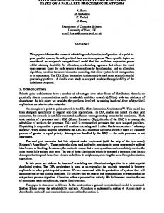
Figure 1: Modeling the Prefetch Mechanism.

a local disk, a remote distributed storage system, or it could generated dynamically by a simulation. B. Prefetching Framework In this section, we present a general framework (illustrated in Figure 1(a)), that describes prefetching in our system. Requests are moving top down while responses move bottom up. The client communicates exclusively with the intermediate storage which we illustrate as Upper Communication in Figure 1(a). The intermediate storage ensures the client’s requirements are met while serving its requests by sending data it stores locally. The Lower Communication Box in Figure 1(a), represents the communication between the intermediate storage and the data store. The intermediate storage prefetched data from the data store that later will be used to serve the client’s requests. The data store exclusively communicates with the intermediate storage and its role is to deliver the requested data to the intermediate storage. This generic framework successfully characterizes prefetching solutions while it abstracts system details allowing designers of clean and easy algorithms with relatively simple proofs (an example of which is illustrated in this paper). Our framework provides a guideline on how to construct prefetching solutions in “any” system. To do so, it purposefully hides system details such as how data and requests are moving through the Upper and Lower Communication and how processing capabilities and client restrictions are described. Upper and Lower Communication are treated as black boxes which ensure communication between system components. IV. D EFINITION OF P REDICTACLE P REFETCHING In this section, given our system architecture, we will formally describe the problem of predictable prefetching. Our goal is to meet the client’s requirement by ensuring that the intermediate storage has enough data when the client needs it. In more detail, when the client requests some data, we need to ensure that these data exist in the intermediate storage. Otherwise, the client would have either to wait or to access the data store which is what we avoid

by our prefetching solutions. Since the intermediate storage has finite space it is important to ensure that we always have updated the data in the intermediate storage with what is needed by the client at each time. We formalize this requirement by the minimum target consumption property: Minimum Target Consumption The data stored in the intermediate storage at each time suffice to provide responses to any request that the client can perform at that time. At a high level, to perform predictable prefetching we need to enforce the minimum target consumption without violating any other system restrictions described below. The client, intermediate storage, and data store each have their own characterization of performance described by their ability to consume or produce operations over (possibly different) units of time. We refer to those as processing bounds. Finally, there may be different requirements characterizing the time data takes to move between the components that we refer to as latency bounds. Predictable Prefetching Problem Given a workload whose accesses are known by the system in advance, processing bounds, and latency bounds, we will specify when to allow the client to start consuming and how should the intermediate storage prefetch data from the data store so that the Minimum Target Consumption is met at all times. Additionally to predictable prefetching we are aiming at solutions that do not block due to lack of space. Blocking of system components is undesirable because it can introduce dependencies on the time it takes for data to propagate throughout the system. These dependencies are difficult to compute, which would make it challenging to provide predictable end-to-end behavior. For those reasons, we would like non-blocking solutions to predictable prefetching, allowing simple composition with other system components across the system. In our system non-blocking would mean that system components are not blocking due to lack of resources to store data (or data to be consumed). In particular, the intermediate storage is allowed to stop producing/consuming operations only as specified by the prefetching algorithm (for example to avoid overflow of the buffer). Similarly, the data store is allowed to perform according to its processing bounds while it never stops due to lack of buffer space. However, it is allowed to stop at will. More formally, we are interested in solutions for the following problem: Non-blocking Predictable Prefetching Problem An algorithm that solves predictable prefetching is non-blocking if the intermediate storage and data store never block due to lack of buffer space. We refer to prefetching algorithms to be solutions to the non-blocking predictable prefetching problem.

V. E XTENSIONS TO RAD–FLOWS M ODEL In this section, we describe the way we model system specifications such as processing capabilities of system components, requirements of applications, and communication between system components. We use this model to later prove correctness of our solutions. Our model is an extension of RAD-FLOWS first presented in [4] that can be used to characterize worst case costs of data flow between components with different processing capabilities. We will show how we can use RAD-Flows to provide sufficient details that have been abstracted by our framework presented in Section III. In particular, in Subsection V-A, we describe the metrics with which system components express their processing capabilities and requirements. In Subsection V-B, we describe how to model communication between system components abstracted by our framework as Upper/Lower Communication (Figure 1(a)). A. RAD Processing Capabilities The RAD (Resource Allocation/Dispatching) model initially was introduced to manage CPU [12] and later extended to manage disks [2], [3]. The model provides the foundations for predictable resource management, decoupling how much resource is needed, from when those resources are needed. The model initially introduced device time utilization as the metric for guaranteed performance. This makes sense for system components such as disk and CPU, but for buffers the RAD metric is rate of operations that can be produced or consumed and the period (time) when this rate must be enforced. The periods are fixed intervals of time that are characterized by their fixed length. According to RAD for buffers, if a node produces (or consumes) operations with rate r over periods of length p, then up to rp operations are produced (or consumed) during any period. Although consumption can happen at any time throughout the period, the model used to manage the component [2], [3] only guarantees that rp operations are consumed within a period if those operations are available at the beginning of this period. In other words, if those operations aren’t available at the beginning of the period, some of these operations may remain in the buffer for some additional time characterized in [4]. We use RAD (rate and period) to characterize the processing bounds of our system. B. Modeling Communication In this section, we will show how to use RAD-FLOWS to describe the Upper/Lower Communication of our prefetching framework. We will model the Upper and Lower Communication using one common abstraction, the LOOP. The LOOP, introduced in [4], is used to characterize cyclic communication between two predictable tasks, requestor and responder. Both Upper and Lower Communication can be characterized by two flows of data: requests move from the component on top, that we call the requestor to the component on the bottom, that we call the responder.

Responses to those request move in the reverse direction. In our system, the requestor of the Upper Communication is the client and the responder is the intermediate storage. For the Lower Communication, the requestor is the intermediate storage and the responder is the data store. The LOOP is the combination of those two flows, more formally: Loop The loop is an abstraction used to characterize bidirectional communication between two real-time components exchanging data through memory buffers: The requestor, sends requests to the responder which in turn sends a correlated response to the requestor. We model the LOOP using RAD-FLOWS [4]. Each communicating component has some processing capabilities described by RAD. In [4], we have fully analyzed the behavior of flow of operations between components with RAD processing capabilities. The two tools we will use here are called TRANSFER and WAIT. • TRANSFER serves queuing operations (in a FIFO queue) between components with possibly different processing capabilities where one component produces operations while the other consumes them. The producer never blocks due to lack of space but it is allowed to produce operations with a variable rate up to a certain upper bound specified by its processing capabilities. Note that this case, the consumer is allowed to stop if no data is available due to the producer’s possibly reduced production. • WAIT is an extension of the TRANSFER building block which allows data to reside in the buffer after they have been consumed in anticipation of some additional event to happen such as: a) receiving an acknowledgment confirming successful completion of the operation or b) waiting for the application to extract the response out of the buffer. An example would be waiting for an acknowledgement confirming that a write has been stored in the remote storage device. The buffer space needed for the WAIT building block depend on the maximum amount of time the corresponding responses take to arrive (i.e., time to serve the operation on a remote system). In [4], we have analyzed the buffer space needed and the time it would take for operations to flow through TRANSFER and WAIT. Those are expressed as functions of RAD processing rates and periods of the system components involved. The buffer space and time needed by the loop is given by the sum of buffer space and buffer times, respectively of the components (ie., TRANSFERs and WAIT) involved in each loop. Next, we provide examples of different loop models but for all cases we denote BL to be the minimum buffer space needed by the LOOP. We denote TL to be the maximum time between the requestor sends a resquest and it receives the corresponding response. Let TL! be the maximum time after the responder consumes a request until it is able to produce a corresponding response as



  



   

          

    

 

 

 

  





     







   





    

Figure 2: Loop. Modeling bidirectional communication.

iillustrated in Figure 2. Finally, as proved in [4], the LOOP does not block any of its components involved because it is constructed by TRANSFERs and WAITs that have the same non-blocking property. Next, we present special cases of the LOOP given certain common practical scenarios. The loop can be used to model various types of communications as shown in Figure 2. We present three loops that characterize the behavior between communicating tasks based on the type of medium used to store the data and the amount of time needed to turn a request into a response. The In Memory Loop is used to model local access where the data is already stored in a memory buffer used to deliver responses. In this model, requests are turned into responses immediately, as they are already available in the memory buffer. The Short Term Loop is used to model slower accesses to local store, such as a disk or flash storage. In this model, requests are turned into responses within the time bounds characterized by the period of the component under the loop (i.e., disk). Note that production from this component happen with the same rate and period as its consumption. The Long Term Loop is used to model accesses to operations that may take some time to complete. The latency bound TL! characterizes the maximum bound to turn a request into a response in the underlying system components after the request has been consumed by the component under the LOOP. Note that production of responses may occur with a different rate and period than consumption of requests. VI. RAD–FETCH M ODEL In this section, we introduce the RAD–FETCH model, and describe the behavior of each of the system components. The RAD–FETCH model is a general framework

characterizing a class of prefetch algorithms and system configurations. RAD-FETCH is described based on three parameters: prebuffering time, OnFetch, and OffFetch. To describe particular instances of algorithms based on RADFETCH model we need to provide particular values for those three functions. An example of such algorithm is given in Section VII. RAD-FETCH can be used as part of a feasibility test during admission control of a system to decide whether a particular instance of a system configuration can satisfy client’s performance requirements. The RAD-FETCH model is derived by our general prefetch framework (Section III) combined with the LOOP. A. Characterizing Processing Capabilities and Latency Processing bounds are all expressed as the RAD processing capabilities of producing and consuming operations. The client can produce requests with maximum rate rc and period pc (RADc ) and consume operations (extract data from the intermediate storage) with maximum rate rc! and period p!c (RAD!c ). Note the client may stop consuming operations. Therefore, some extra space may be needed to hold responses from the point where they become available for consumption until they are actually consumed. This is a function of the maximum number of outstanding operations the client is allowed to have. The intermediate storage receives requests from the client with maximum rate rI and period pI (RADI ) and it sends data to the client with the same processing capabilities and T!L = 0. This is because, we model access to a local storage memory by characterizing production and consumption with the same performance capabilities and no time separation between these two events (In Memory or Short Term LOOP). The intermediate storage sends requests to the data store with maximum rate rI! and period p!I (RAD!I ) and receives data from the data store with maximum rate rI!! and period p!!I (RAD!!I ). Finally, the data store receives requests from the intermediate storage with maximum rate rs and period ps (RADs ) and sends data to the intermediate storage with maximum rate rs! and period p!s (RAD!s ). The client’s latency bounds require that it must receive a corresponding response to a request within Tmax time. B. Characterizing Component’s Behavior The Upper and Lower Communication of our prefetching framework (Figure 1(a)) is modeled by LOOPs as illustrated in Figure 1(b). In particular, the top LOOP is either a In Memory or Short Term LOOP and the one on the bottom can be any among all possible LOOPS of Figure2. We will describe the behavior of each of the system components (i.e., client, intermediate storage and data store). The client’s behavior is a given to our problem: The client produces requests and consumes responses given its processing bounds. Even though responses may be available by the system to the client, those will have to be consumed by the client according to its processing bounds (rate and period

of consumption). Since the client’s consumption happens asynchronously compared to its production of requests, there may be some outstanding operations (i.e. number of requests that has been produced by the client, but not consumed by the client yet) at any given point in time. We assume that there is an upper bound on those that we denote Omax . We can calculate that additional space by adding a WAIT component in the LOOP between the client and the intermediate storage. Contrary to the client, the production of data by the data store is directly derived by its consumption of requests. Production of responses from the intermediate storage to the client is derived directly by the consumption of requests. The Data Store produces responses to operations that has been previously consumed consumed with a maximum separation in time TL! after consumption of the request. It remains to describe the behavior of the intermediate storage. The production of requests of the intermediate storage is under the control of the system. In particular, the intermediate storage operates in three phases: Prebuffering Phase, Steady Phase, and Final Phase. During the Prebuffering Phase, the intermediate storage accumulates data from the data store before the client is allowed to start consumption. The amount of data accumulated in the intermediate storage is expressed by variable DataInCache in Figure VI-B. Once these data is accumulated then the client is allowed to start consumption and it does so by moving into the Steady Phase (Figure VI-B.). In the Steady Phase we ensure that there is always enough data in the intermediate storage but not infinitely many. To ensure that, the intermediate storage starts prefetching when the data in the cache goes below a certain threshold denoted as OnFetch in Figure VI-B. This is expressed in line 4 of Figure VI-B. Similarly, we stop prefetching when the data in the cache exceeds another threshold denoted as OffFetch in Figure VI-B. This is expressed in line 7 of Figure VI-B. When the intermediate storage wants to prefetch data it sends r!I p!I requests every p!I . When the intermediate storage stops prefetching then it stops sending requests. The Steady Phase is repeated indefinitely until the end of the workload during which we move to the Final Phase. During the Final Phase the system stops prefetching data and the client consumes all remaining data. VII. RAD-FETCH A LGORITHM In this section, we present our prefetching algorithm. This algorithm is based on the RAD-FETCH model. Recall that this model provides a general framework of a class of prefetching algorithms. To derive a specific algorithm we just need to provide specific values for the parameters that are not evaluated in RAD-FETCH model. The algorithm works exactly as specified in Section VI-B when we replace the RAD-FETCH parameters as follows: The parameter OnFetch corresponds to data size that trigger starting prefetching. As we will show in our proof

Algorithm VI.1 Steady Phase of prefetch algorithm 1: while more data is available to consume do 2: wait until the beginning of the period (p!I ) 3: if DataInCache < OnFetch then 4: turn prefetch ON 5: end if 6: if DataInCache >= OffFetch then 7: turn prefetch OFF 8: end if 9: if prefetch is ON then 10: fetch one period worth of data (r!I p!I ) 11: end if 12: end while

of correctness in the next section, it suffices that OnFetch contains rc pc data plus the maximum amount of data that can be removed from the intermediate storage within a time interval of length p!I + TL + e, where e is the smallest possible value that forces this interval to start and end at the beginning of some period p!I . It is easy to calculate that: " ! ! pI + TL ! pI − (p!I + TL ) (1) e= p!I " ! ! pI + TL + e )rI pI (2) OnFetch = rc pc + ( pI The parameter OffFetch triggers the intermediate storage to stop prefetching and it is evaluated as follows: ! " max (TL , p!I ) OffFetch = OnFetch + ( + 1)rI pI pI

(3)

Finally, the prebuffering time chatacterizes the time it will elapse before the client can start producing operations. During that time the intermediate storage is prefetching data as explained in detail in Section VI-B. Prebuffering Time = TL + p!I + e +

!

" OnFetch ! pI rI! p!I

(4)

VIII. T HEORETICAL E VALUATION OF RAD–FETCH Clients with hard performance requirements have to wait until some data is fetched by the intermediate storage prior to starting their execution as formally shown in [4]. We described this initial phase as prebuffering phase in RADFETCH. The first question to answer by our analysis is how much time the client has to wait before it can start producing its operations and how much data should the intermediate storage prefetch during the prebuffering phase. Recall that the former is the prebuffering time and the later is the prebuffering space. In Theorem 8.8 we show that the value of prebuffering time given by Equation 4 suffices for our RAD-FETCH algorithm to work correctly. Prebuffering space is calculated in Theorem 8.10.

During the Steady Phase (after the prebuffering phase), the intermediate storage starts and stops prefetching upon need based on: OnFetch and OffFetch. Providing exact values for those parameters answers the question of when to turn on and off prefetching to meet the applications requirements without overflowing/underflowing the buffer in the intermediate storage. In Theorem 8.8 we show that the value of OnFetch and OffFetch given by equations 2 and 3, respectively suffice for correctness. The rest of the section is organized as follows: In Subsection VIII-A, we show that our RAD-FETCH algorithm (Section VII), solves the non-blocking predictable prefetching problem. In Subsection VIII-B, we analyze how much buffer space is needed by our prefetching algorithm. The buffer space needed is calculated as a function of the RAD processing capabilities of the system components. A. Correctness of RAD-FETCH Algorithm Our goal is to ensure the minimum target consumption without blocking of the system components. To do this, we need to have enough available data in the intermediate storage so that the client can perform its operations by exclusively accessing the intermediate storage. In our model, the client may request up to rc pc operations every period pc . Hence, in our model, the minimum target consumption translates to having the maximum data (i.e., rc pc ) that the client can request at the beginning of each period pc . Hence, for our RAD-FETCH algorithm suffices to ensure RAD– TARGET: Property 8.1 (RAD–TARGET): The intermediate storage has rc pc data available at the beginning of each period pc after the client is allowed to start requesting data (i.e., after the prebuffering phase). For RAD-FETCH to support correct prefetching algorithms, we need to impose some restrictions of the rates of the components (properties 8.2,8.3, 8.4). Property 8.2 is necessary as the client must be able to consume operations at least as fast as it requests them, to avoid buffer overflow. Property 8.3 ensures that the intermediate storage’s rate of prefetching requests from the data store is larger than or equal to the rate at which requests may be coming out of the intermediate storage to avoid buffer underflow. Finally, Property 8.4 ensures that the data store can produce data to the intermediate storage fast enough by matching the rate of consumption of requests by the intermediate storage. Property 8.2: The maximum rate of production of the client is smaller or equal to its maximum rate of consumption: rc ≤ rc! . Property 8.3: The maximum rate of refilling the cache should be larger or equal to the maximum # $ rate of emptying ! ! the cache. It suffices that: rI pI ≥ ( ppI! + 1)rI pI . I Property 8.4: The maximum rate of production of data by the data store must be larger than or equal to its rate of consumption of the corresponding requests: rs ≤ rs!

Given our rate assumptions (properties 8.2, 8.3, 8.4), formal correctness of our algorithm follows in Theorem 8.8. We start with some preliminary lemmata. Lemma 8.5: If the intermediate storage performs prefetching during a period of time while data are not removed from the intermediate storage, then after p!I +TL +e time has elapsed, the intermediate storage will be storing at least (additional) rI! p!I data by the beginning of each period p!I . Proof: While the intermediate storage performs prefetching it sends its maximum requests rI! p!I per period p!I . Those requested travel through the LOOP and data arrives back from the data store within the LOOP’s latency TL . Since there is no control on where within a period p!I the intermediate storage will issue requests, it may take up to time TL + p!I to start receiving requested data. At the beginning of the next p!I period (i.e., after TL + p!I + e time) then data is guaranteed to be consumed (hence stored) by the intermediate storage and in the worst case those arrive at the beginning of each period p!I . Lemma 8.6: At the end of the # prebuffering $ phase (i.e., p!I ), there are after prebuffering time TL + p!I +e+ OnFetch rI! p!I at least OnFetch data available in the intermediate storage. Proof: The prebuffering phase lasts for prebuffering $ # ! . During that time the p time TL + p!I + e + OnFetch ! ! I rI pI intermediate storage continually performs prefetching and no data come out of the intermediate storage since the client has not started requesting data. Then from Lemma 8.5, we know that rI! p!I data will be stored in the intermediate storage by the beginning of every p!I period after ≤ TL + p!I + e time has elapsed. Since $ the prebuffering phase continues for another # OnFetch periods of length p! , then by the end of the I rI! p!I period we $are guaranteed to have in the intermediate storage # OnFetch r! p! ≥ OnFetch data. I I rI! p!I Lemma 8.7: During the Steady Phase, the intermediate storage maintains at least rc pc data at all times. Proof: By Lemma 8.6, because the steady phase starts at the end of the prebuffering phase, at the beginning of the intermediate storage there is at least OnFetch data available in the intermediate storage. We will divide the Steady Phase into two types of execution fragments separated by starting and stopping prefetching. First, let’s consider an execution fragment between starting prefetching (where we have OnFetch data available) and stopping prefetching (when we have OffFetch data available). During the first p!I + TL + e time of this execution fragment, the intermediate storage may not receive any data as it may take that much time until the requests travel through the loop and data appear as a response. This value is calculated to be the beginning of a period p!I after the ! latency of the loop plus a period $ elapsed. During that # ! pI has pI +TL +e + 1)rI pI data removed time there can be at most ( pI from the intermediate storage, because data is moved out

with rate rI and period pI . In the worst case, no data has been added during that period. At $ the end of that period, # ! pI +TL +e + 1)rI pI = rc pc data left there will be OnFetch − ( pI in the intermediate storage. But at the beginning of every subsequent period there will be a gain of at least rI! p!I data added to the intermediate storage by Lemma 8.5. Hence until the intermediate storage stop prefetching, we guarantee that for the next periods p!I there is at least additional rI! p!I data stored per p!I . By Assumption 8.3, during those periods we will have no loss of data since what we are guaranteed to gain in size of data in the intermediate storage (i.e. rI! p!I ) at the beginning of each period p!I is larger or equal to the maximum data that# the$ intermediate storage can loose during that period (i.e. ( ppI! + 1)rI pI ). If OffFetch is reached at I any time during the intervals considered above then dditional data accumulated than the above calculated minimum values. Hence at all times we never had less than rc pc between starting prefetching and stopping prefetching. It remains to consider the execution fragments between stopping prefetching and starting prefetching. For this case it is trivial to see that we have at least rc pc data available in the intermediate storage because by definition of this execution fragment during that time there is no less than OnFetch data available in the intermediate storage and OnFetch is larger than rc pc . Theorem 8.8: Given the rate assumptions (Properties 8.2, 8.3, and 8.4) our RAD-FETCH algorithm solves the nonblocking predictable prefetching problem. Proof: First, we will show how we ensure the min target consumption. Given RAD-FETCH, to ensure the minimum target consumption (Property IV) it suffices to ensure the RAD–TARGET property 8.1, as explained at the beginning of this section. RAD-TARGET is ensured by Lemma , which ensures that the required rc pc data are available in the intermediate storage at all times. Second, given that the system has enough buffer space (as calculated in Subsection VII) to support our RAD–FETCH algorithm, the latency bound Tmax of the client is met given that it is larger or equal to the latency of the loop used for Upper Communication. This is because, the minimum target consumption ensures that all responses to the client can be served through the intermediate storage at all times. Finally, our RAD-FETCH algorithm is non-blocking because it is build upon RAD-FLOWS components that are non-blocking either as shown in [4]. In particular, all involved consumers and producers never block due to lack of space which is proved in RAD–FLOWS [4]. B. Analysis of Buffer Space of RAD-FETCH Algorithm In this section, we calculate the minimum buffer space that suffices for our RAD-FETCH algorithm. To calculate that value we add the space needed by the 2 LOOPs (i.e., 2BL ) to the space needed by the algorithm run by the intermediate storage (which is the maximum data accumulated duringvprebuffering and steady phase).

Lemma 8.9: It takes at least time TL after stopping prefetching until the intermediate storage starts prefetching. Proof: For the intermediate storage to stop $ # prefetching, max (TL ,p!I ) + it has in its storage OffFetch = OnFetch + ( pI 1)r p data. For it to start prefetching it must loose #I I $ max (TL ,p!I ) ( + 1)rI pI data so that it meets the triggering pI condition of prefetching (i.e., there are only OnFetch data stored. The data is removed from the intermediate storage with RAD processing capabilities rI , #pI (i.e., at $most rI pI max (TL ,p!I ) every pI ). Hence, to loose at least ( + 1)rI pI pI data, at least max (TL , pI ) time has elapsed and as a result, at least TL time has elapsed. We conclude that between stopping and starting prefetching at least TL time has elapsed and the Lemma follows. Theorem 8.10: The prebuffering space is at least OnFetch and at most (prebuffering time)rI! . Proof: The prebuffering space is at least OnFetch follows directly from Lemma 8.6. The maximum data accumulated during the prebuffering phase is bounded by the maximum data that the intermediate storage can request during that time. Since the intermediate storage requests rI! p!I data per p!I , then the maximum prebuffering space is rI! p!I multiplied by the number of p!I periods that can fit in prebuffering time. Since prebuffering time is a multiple of such periods then the maximum data is prebuffering time multiplied by the rate rI! . Theorem 8.11: It suffices to #have 2BL + $ max ((prebuffering time)rI! , OffFetch + ( TpL! + 1)rI! p!I ) I buffer space available for the RAD-FETCH algorithm to work correctly. Proof: Since there are two loops involved in the RAD– FETCH algorithm, we need at least 2BL buffer space to account for those two loops. Next we calculate how much additional space is needed by the intermediate storage. This is given as the maximum of the space needed during prebuffering phase (which is prebuffering time)rI! , and during the steady phase. Next $ show that during the steady phase # we at most OffFetch + ( TpL! + 1)rI! p!I ) buffer space is needed I and hence the theorem follows. During steady phase, when prefetching is on the data stored in the intermediate storage is less than or equal to OffFetch. Once the OffFetch threshold is met no more data is prefetched for the next TL time (by Lemma 8.9). During that time the intermediate storage can receive data that is still in transit (requested before stopping prefetching and not received yet). This is bounded by at most the maximum amount of data that the intermediate storage can request within a period of length TL . Since the intermediate storage ! ! ! can request at most # rI$pI operations per period pI and there can be at most ( TpL! + 1) periods p!I overlapping TL the I # $ maximum data in transit is equal to ( TpL! + 1)rI! p!I . I

IX. C ONCLUSION AND F UTURE W ORK We have presented the RAD–FETCH model that characterizes predictable prefetching using RAD–FLOWS. This model supports hard real–time applications. The main contribution of our work is a full analysis that describes how to prefetch data in order to ensure the application’s requirements without violating the system capabilities. Without our model in place prefetching could result in unnecessary overprovisioning. More importantly, there will be no assurance of the bound on the executiom time of the workload, needed for hard real–time applications. As future work, we plan to extend the RAD–FLOWS to model other cache mechanisms such as writeback and cache hits. R EFERENCES [1] A. Verma, K. Voruganti, R. Routray, and R. Jain, “Sweeper: an efficient disaster recovery point identification mechanism,” in Proceedings of the 6th USENIX Conference on File and Storage Technologies, ser. FAST’08, 2008, pp. 20:1–20:16. [2] A. Povzner, T. Kaldewey, S. Brandt, R. Golding, T. M. Wong, and C. Maltzahn, “Efficient guaranteed disk request scheduling with fahrrad,” SIGOPS Oper. Syst. Rev., vol. 42, no. 4, pp. 13–25, 2008. [3] T. Kaldewey, T. M. Wong, R. Golding, A. Povzner, S. Brandt, and C. Maltzahn, “Virtualizing disk performance,” Real-Time and Embedded Technology and Applications Symposium, IEEE, vol. 0, pp. 319–330, 2008. [4] R. Pineiro, K. Ioannidou, S. Brandt, and C. Maltzahn, “Radflows: Buffering for predictable communication,” in Proceedings of the 17th IEEE Real Time on Embedded Technology and Applications Symposium. Washington, DC, USA: IEEE Computer Society, 2011. [5] R. Wilhelm, J. Engblom, A. Ermedahl, N. Holsti, S. Thesing, D. Whalley, G. Bernat, C. Ferdinand, R. Heckmann, T. Mitra, F. Mueller, I. Puaut, P. Puschner, J. Staschulat, and P. Stenström, “The worst-case execution-time problem– overview of methods and survey of tools,” ACM Trans. Embed. Comput. Syst., vol. 7, pp. 36:1–36:53, May 2008. [6] H. Ramaprasad and F. Mueller, “Bounding worst-case data cache behavior by analytically deriving cache reference patterns,” in Proceedings of the 11th IEEE Real Time on Embedded Technology and Applications Symposium, 2005, pp. 148–157. [7] Y. Ding and W. Zhang, “Loop-based instruction prefetching to reduce the worst-case execution time,” IEEE Transactions on Computers, vol. 59, pp. 855–864, 2010. [8] J. Yan and W. Zhang, “Analyzing the worst-case execution time for instruction caches with prefetching,” ACM Trans. Embed. Comput. Syst., vol. 8, pp. 7:1–7:19, January 2009. [9] M. Lee, S. L. Min, and C. S. Kim, “A worst case timing analysis technique for instruction prefetch buffers,” in Selected papers of the short notes session on Euromicro ’94, 1994, pp. 681–684.

[10] X. Zhuang and H.-H. S. Lee, “Reducing cache pollution via dynamic data prefetch filtering,” IEEE Trans. Comput., vol. 56, pp. 18–31, January 2007. [11] J. Reineke, D. Grund, C. Berg, and R. Wilhelm, “Timing predictability of cache replacement policies,” Real-Time Syst., vol. 37, pp. 99–122, November 2007. [12] S. A. Brandt, S. Banachowski, C. Lin, and T. Bisson, “Dynamic integrated scheduling of hard real-time, soft real-time and non-real-time processes,” in Proceedings of the 24th IEEE Real-Time Systems Symposium (RTSS 2003), Dec. 2003, pp. 396–407. [13] S. Brandt, C. Maltzahn, A. Povzner, R. Pineiro, A. Shewmaker, and T. Kaldewey, “An integrated model for performance management in a distributed system,” OSPERT, 2008. [14] B. S. Gill and L. A. D. Bathen, “Amp: adaptive multi-stream prefetching in a shared cache,” in Proceedings of the 5th USENIX conference on File and Storage Technologies, 2007, pp. 26–26. [15] A. J. Smith, “Cache memories,” in ACM Comput. Surv, 1982, pp. 473–530. [16] S. Harizopoulos, C. Harizakis, and P. Triantafillou, “Hierarchical caching and prefetching for high performance continuous media servers with smart disks,” IEEE Concurrency, vol. 8, p. 2000, 2000. [17] B. S. Gill and D. S. Modha, “Sarc: sequential prefetching in adaptive replacement cache,” in Proceedings of the annual conference on USENIX Annual Technical Conference, ser. ATEC ’05, 2005, pp. 33–33. [18] F. Dahlgren, M. Dubois, and P. Stenstrom, “Fixed and adaptive sequential prefetching in shared memory multiprocessors,” in Proceedings of the 1993 International Conference on Parallel Processing - Volume 01, ser. ICPP ’93, 1993, pp. 56–63. [19] T.-F. Chen and J.-L. Baer, “Reducing memory latency via non-blocking and prefetching caches,” in Proceedings of the fifth international conference on Architectural support for programming languages and operating systems, ser. ASPLOS-V, 1992, pp. 51–61. [20] S. Lim and M. H. Kim, “A real-time prefetching method for continuous media playback,” Database and Expert Systems Applications, International Workshop on, vol. 0, p. 889, 1999. [21] S. Oh, B. Kulapala, A. Richa, and M. Reisslein, “Continuoustime collaborative prefetching of continuous media,” Broadcasting, IEEE Transactions on, vol. 54, no. 1, pp. 36 –52, mar. 2008.